Dynamic Multiscaling in Turbulence

Abstract

We give an overview of the progress that has been made in recent years in understanding the dynamic multiscaling of homogeneous, isotropic turbulence and related problems. We emphasise the similarity of this problem with the dynamic scaling of time-dependent correlation functions in the vicinity of a critical point in, e.g., a spin system. The universality of dynamic-multiscaling exponents in fluid turbulence is explored by detailed simulations of the GOY shell model for fluid turbulence.

1 Introduction

The statistical properties of fully developed, homogeneous, isotropic turbulence are often characterised by velocity structure functions, which are averages of the differences of fluid velocities at two points separated by a distance $r$ (a precise definition is given below). If $r$ lies in the inertial range of scales that lie between the large length scale $L$, at which energy is pumped into a turbulent fluid, and the small dissipation scale $\eta_{d}$, at which viscous dissipation becomes significant, these structure functions scale as a power of $r$, in a manner that is reminiscent of the algebraic behaviour of correlation functions at a critical point in, say, a spin system. This similarity between the statistical properties of homogeneous, isotropic turbulence and a system at a critical point is well known; and its elucidation for equal-time structure functions has been the subject of many papers: It turns out that the simple scaling we are accustomed to at most critical points must be generalised to multiscaling in turbulence; i.e., an infinity of exponents is required to characterise the inertial-range behaviours of structure functions of different orders [1].

The scaling behaviour of correlation functions at a critical point [2] is associated with the divergence of a correlation length $\xi$ at the critical point; e.g., in a spin system $\xi\sim\bar{t}^{\nu}$ if the field $H=0$, where the reduced temperature $\bar{t}\equiv(T-T_{c})/T_{c}$, $T$ is the temperature, $T_{c}$ the critical temperature, and $\nu$ is an equal-time critical exponent that is universal (for systems in a given universality class). In the vicinity of a critical point the relaxation time $\tau$, which can be determined from time-dependent correlation functions, scales as follows:

$$\tau\sim\xi^{z}.$$ (1)

This is known as the dynamic-scaling Ansatz via which we define $z$, the dynamic-scaling exponent. Over the past few years there has been considerable progress  [3, 4, 5, 6, 7, 8, 9] in developing the analogue of such a dynamic-scaling Ansatz for time-dependent structure functions in homogeneous, isotropic turbulence. We give an overview of this work on dynamic mutiscaling in turbulence. We show, in particular, that (a) an infinity of dynamic-multiscaling exponents is required here, (b) these exponents depend on the precise way in which relaxation times are extracted from time-dependent structure functions, and (c) that dynamic-multiscaling exponents are related by linear bridge relations to equal-time multiscaling exponents.

The remaining part of this paper is organised as follows: Section 2 contains an introduction to the multiscaling of equal-time structure functions in fluid turbulence. Section 3 is devoted to the dynamic multiscaling of time-dependent structure functions. In Sect. 4 we introduce the GOY shell model [1, 10, 11] for fluid turbulence and give the details of our numerical studies of this model. Section 5 gives representative results from our simulations for time-dependent structure functions for the GOY shell model with conventional viscosity; we also present new results with hyperviscosity and show explicitly that dynamic multiscaling exponents are independent of the type of viscosity we use. We end with concluding remarks about the possibility of experimental verifications of our predictions and generalizations to other types of turbulence such as passive-scalar turbulence[12].

2 Equal-time Multiscaling

Fluid flows are described by the Navier-Stokes equation for the velocity field ${\bf u}({\bf x},t)$ at point ${\bf x}$ and time $t$:

$$\partial_{t}{\bf u}+{\bf u}.\nabla{\bf u}=-\nabla P+\nu_{0}\nabla^{2}{\bf u}+{\bf f};$$ (2)

we consider low-Mach number flows that are nearly incompressible and so equation (2) must be augmented by the incompressibility constraint

$$\nabla.{\bf u}=0,$$ (3)

which can be used to eliminate the pressure $P$ in equation (2); we choose the uniform density $\rho=1$; $\nu_{0}$ is the kinematic viscosity; and for decaying turbulence the external force ${\bf f}$ is zero. Turbulence occurs when the Reynolds number $Re\equiv(\ell v)/\nu_{0}$ is large; here $\ell$ and $v$ are characteristic length and velocity scales of the flow.

The chaotic nature of turbulence has led to a natural statistical description of the velocity field in terms of velocity structure functions. For instance, we can define the order-$p$, equal-time, structure function for longitudinal velocity increments $\delta u_{\parallel}({\bf x},{\bf r},t)\equiv[{\bf u}({\bf x}+{\bf r},t)-{\bf u}({\bf x},t)].{\bf r}/r$ as follows:

$${\cal S}_{p}(r)\equiv\left\langle[\delta u_{\parallel}({\bf x},{\bf r},t)]^{p}\right\rangle\sim r^{\zeta_{p}};$$ (4)

the power-law dependence on $r$, which defines the exponent $\zeta_{p}$, holds for $L\ll r\ll\eta_{d}$; and the angular brackets indicate an average over either the statistical steady state, for forced turbulence, or statistically independent initial conditions, for decaying turbulence.

In contrast with the scaling behaviour of correlation functions at conventional critical points in equilibrium statistical mechanics, in turbulence the structure functions ${\cal S}_{p}(r)$ do not exhibit simple scaling forms: Experimental and numerical evidence suggests that ${\cal S}_{p}(r)$ show multiscaling, with $\zeta_{p}$ a nonlinear, convex, monotone increasing function of $p$ [1]. The 1941 theory of Kolmogorov (K41)  [13, 14] yields simple scaling with $\zeta_{p}^{K41}=p/3$; the measured values of $\zeta_{p}$ deviate significantly from $\zeta_{p}^{K41}$ for $p>3$; and for $p=3$ we have the exact von Kármán-Howarth [1] result $\zeta_{3}=1$.

Even though the K41 phenomenology fails to capture the multiscaling of the equal-time structure function ${\cal S}_{p}(r)$, it provides us with important conceptual underpinnings for studies of homogeneous, isotropic turbulence. In particular, the exponents $\zeta_{p}^{K41}$ are universal in the sense that they do not depend on the details of the dissipation, i.e., the viscosity. (Of course measurements should be made far away from boundaries so that the flow satisfies the conditions of homogeneity and isotropy.) This suggestion of power-law scaling with universal scaling exponents was made for turbulence a few decades before it was appreciated fully in the context of critical phenomena.

The universality of the exponents $\zeta_{p}$ holds even if we go beyond K41 phenomenology. Let us first examine the dependence of these exponents on the dissipation mechanism. In numerical simulations it is possible to introduce a hyperviscosity $\nu_{\alpha}$ by replacing the viscous term $\nu_{0}\nabla^{2}{\bf u}$ in equation (2) by $\nu_{\alpha}\nabla^{2+\alpha}{\bf u}$; here $\alpha\geq 0$ determines the degree of hyperviscosity; and $\alpha=0$ yields normal viscous dissipation. Some early shell-model studies [15, 16, 17] suggested that the exponents $\zeta_{p}$ depend on $\alpha$. But subsequent direct numerical simulations (DNS) [18] of equations (2-3) and numerical studies of a shell model [19] for turbulence have argued against this. Our results are consistent with these later studies.

The exponents $\zeta_{p}$ do not seem to depend on whether they are measured in statistically steady, forced turbulence or in decaying turbulence. Numerical evidence for this universality has been provided by the shell-model studies of Ref. [20].

In the remaining Sections of this paper we will show how to generalise the dynamic-scaling Ansatz (1) to account for multiscaling in turbulence. Our discussion will be based on earlier studies [3, 6] and the work carried out in our group [4, 5]. We will then examine the universality of the dynamic-multiscaling exponents in fluid turbulence, i.e., we will explore their dependence on (a) the hyperviscosity parameter $\alpha$ and (b) the type of turbulence (statistically steady as opposed to decaying).

3 Dynamic Multiscaling

The dynamic scaling of time-dependent correlation functions at a critical point in an equilibrium system was systematised soon after the scaling of equal-time correlation functions. The analogous development for homogeneous, isotropic turbulence has been carried out recently [3, 4, 5, 6, 7]. We summarise the essential points here before presenting our new results. A naïve extension of K41 phenomenology to time-dependent structure functions yields a dynamic exponent $z^{K41}=2/3$ for all orders $p$. Two improvements are required to go beyond this K41 result: (a) We must account for the multiscaling of velocity structure functions. (b) We must distinguish between structure functions of Eulerian and Lagrangian velocities; the former yield trivial dynamic scaling with $z^{\cal E}=1$, for all $p$, since the mean flow (or the flow of the largest eddy) directly advects small eddies and so temporal and spatial separations are related linearly by the mean flow velocity; nontrivial dynamic multiscaling can be anticipated, therefore, only for Lagrangian [21] or quasi-Lagrangian [6] velocity structure functions. The latter are defined in terms of the quasi-Lagrangian velocity ${\bf\hat{u}}$ that is related to its Eulerian counterpart $\bf{u}$ as follows:

$${\bf\hat{u}}({\bf x},t)\equiv{\bf u}[{\bf x}+{\bf R}(t;{\bf r_{0}},0),t],$$ (5)

with ${\bf R}(t;{\bf r_{0}},0)$ the position at time $t$ of a Largrangian particle that was at ${\bf r_{0}}$ at time $t=0$. Equal-time, quasi-Lagrangian velocity structure functions are the same as their Eulerian counterparts [22].

The order-$p$, time-dependent, structure function, for longitudinal, quasi-Lagrangian velocity increments is [3, 4]

$${\mathcal{F}}_{p}(r,\{t_{1},\ldots,t_{p}\})\equiv\left\langle[\delta\hat{u}_{\parallel}({\bf x},t_{1},r)\ldots\delta\hat{u}_{\parallel}({\bf x},t_{p},r)]\right\rangle.$$ (6)

Since we are interested in scaling behaviours, we restrict $r$ to the inertial range, consider, for simplicity, $t_{1}=t$ and $t_{2}=\ldots=t_{p}=0$, and denote the structure function (6) by ${\mathcal{F}}_{p}(r,t)$. Given ${\mathcal{F}}_{p}(r,t)$, there are different ways of extracting time scales. For example, we can use the following order-$p$, degree-$M$ integral- and derivative-time scales that are defined, respectively, as [4]

$${\cal T}^{I}_{p,M}(r)\equiv\biggl{[}\frac{1}{{\mathcal{S}}_{p}(r)}\int_{0}^{\infty}{\mathcal{F}}_{p}(r,t)t^{(M-1)}dt\biggl{]}^{(1/M)}$$ (7)

and

$${\cal T}^{D}_{p,M}(r)\equiv\biggl{[}\frac{1}{{\mathcal{S}}_{p}(r)}\frac{\partial^{M}{\mathcal{F}}_{p}(r,t)}{\partial t^{M}}\biggl{|}_{t=0}\biggl{]}^{(-1/M)}.$$ (8)

If the integral in (7) and the derivative in (8) exist we can generalise the dynamic-scaling Ansatz (1) at a critical point to the following dynamic-multiscaling Ansätze for homogeneous, isotropic turbulence [3, 4]:

$${\cal T}^{I}_{p,M}(r)\sim r^{z^{I}_{p,M}};$$ (9)

$${\cal T}^{D}_{p,M}(r)\sim r^{z^{D}_{p,M}}.$$ (10)

These equations define, respectively, the integral- and the derivative-time multiscaling exponents $z^{I}_{p,M}$ and $z^{D}_{p,M}$, which satisfy the bridge relations

$$z^{I}_{p,M}=1+[\zeta_{p-M}-\zeta_{p}]/M,$$ (11)

obtained first in Ref. [3], and

$$z^{D}_{p,M}=1+[\zeta_{p}-\zeta_{p+M}]/M,$$ (12)

obtained in Ref. [4]. These bridge relations follow from a generalisation [3, 4] of the multifractal formalism [1] for turbulence. Here we sketch the arguments that lead to equation (11) for statistically steady turbulence and refer the reader to Refs. [4, 23] for details: We begin by assuming the following multifractal form for the order-$p$ time-dependent structure functions:

$$\frac{{\cal F}_{p}(r,t)}{\hat{u}_{L}^{p}}\propto\int_{I}d\mu(h)\big{(}\frac{r}{L}\big{)}^{3+ph-{\cal D}^{\hat{u}}(h)}{\cal G}^{p,h}(\frac{t}{\tau_{p,h}}).$$ (13)

As in the equal-time multifractal formalism [1], the scaling exponents $h\in{\cal I}\equiv[h_{min},h_{max}]$. Corresponding to each exponent $h$ there is a set ${\bf\Sigma}_{h}\subset{\mathbb{R}}^{3}$, of fractal dimension ${\cal D}^{\hat{u}(h)}$ and with a measure $d\mu(h)$, such that $\delta\hat{u}_{r}({\bf x})/\hat{u}_{L}\sim(r/L)^{h}$ if ${\bf x}\in{\bf\Sigma}_{h}$, with $\delta\hat{u}_{r}({\bf x})\equiv|{\bf\hat{u}}({\bf x+r})-{\bf\hat{u}}({\bf x})|$. We assume furthermore that the scaling function ${\cal G}^{p,h}(\frac{t}{\tau_{p,h}})$ is such that ${\cal G}^{p,h}(0)=1$ and that the characteristic decay time $\tau_{p,h}\sim r/\delta\hat{u}_{r}({\bf x})\sim r^{1-h}$. If we substitute for ${\cal F}_{p}(r,t)$ in equation (9), do the time integral first by a saddle-point method, we obtain the bridge relation (11). Similar calculations lead to (12). A complete discussion of such bridge relations, as well as similar relations for passive-scalar turbulence, can be found in Refs.  [4, 5, 23]. The last of these references also shows that the bridge relations are the same for decaying and statistically steady turbulence.

Given current computational resources, it has not been possible to verify the bridge relations (11-12) by computing quasi-Lagrangian velocities in a direct numerical simulation of the Navier-Stokes equation (2-3) for an incompressible fluid. Thus we must turn to numerical studies of simple shell models of turbulence that we describe in the next Section.

4 The GOY Shell Model

We have carried out extensive numerical simulations to obtain equal-time and dynamic multiscaling exponents for the GOY shell model for fluid turbulence [1, 10, 11]. This shell model is defined on a logarithmically discretized Fourier space labelled by scalar wave vectors $k_{n}$ that are associated with the shells $n$. The dynamical variables are the complex scalar shell velocities $u_{n}(k_{n})$, henceforth denoted by $u_{n}$. The evolution equations for the GOY model are

$$\left[\frac{d}{dt}+\nu_{0}\left(\frac{k_{n}}{k_{d}}\right)^{\alpha}k_{n}^{2}\right]u_{n}=\imath\bigg{[}a_{n}u_{n+1}u_{n+2}+b_{n}u_{n-1}u_{n+1}+c_{n}u_{n-1}u_{n-2}\bigg{]}^{\ast},$$ (14)

where $k_{n}=k_{0}2^{n}\/$, $k_{0}$ = 1/16, complex conjugation is denoted by $\ast$, and the coefficients $a_{n}=k_{n}$, $b_{n}=-\delta k_{n-1}$, $c_{n}=-(1-\delta)k_{n-2}$ are chosen to conserve the shell-model analogues of energy and helicity in the inviscid, unforced limit, and $1\leq n\leq N$. We use the standard value $\delta=1/2$. The second term allows for hyperviscous dissipation with degree $\alpha$ (the case $\alpha=0$ corresponds to conventional viscous dissipation); $k_{d}$ is a large wavenumber whose inverse is comparable to the dissipation length scale; we choose $k_{d}=2^{18}$ and $\alpha=0$ or $\alpha=2$. Since we concentrate on decaying turbulence here, the forcing term, required to drive the system into a statistically steady state, is absent. The logarithmic discretization of Fourier space allows us to reach very high Reynolds numbers in numerical simulations of the GOY model even with $N=22$.

We use a slaved, second-order, Adams-Bashforth scheme  [24, 25] to integrate the GOY-model equations with $N=22$ shells, and, in some representative cases, $N=35$ (this requires a fifth-order scheme  [26] ), with the boundary conditions $u_{n}=0$ for $n\leq 0$ and $n>N$. In our simulations we use $\delta t=10^{-4}$ as the integration time step, and the viscosity $\nu=10^{-7}$ for $\alpha=0$ and $\nu=10^{-6}$ for $\alpha=2$.

The GOY-model equations allow for direct interactions only between nearest- and next-nearest-neighbour shells. By contrast, in the Fourier transform of the Navier-Stokes equation every Fourier mode of the velocity is coupled to every other Fourier mode directly. This direct sweeping, as it is called, leads to the trivial dynamic scaling of Eulerian velocity structure functions (Sect. 3). Since the GOY model does not have direct sweeping in this sense, it is sometimes thought of as a highly simplified quasi-Lagrangian version of the Navier-Stokes equation. Thus we might expect nontrivial dynamic multiscaling for GOY-model structure functions. The equal-time structure functions for this model are

$$S_{p}(k_{n})\equiv\left\langle[u_{n}(t)u^{\ast}_{n}(t)]^{p/2}\right\rangle\sim k_{n}^{-\zeta_{p}},$$ (15)

where the power-law dependence is obtained only if $k_{n}^{-1}$ lies in the inertial range. Three cycles [27] in the static solutions of the GOY model lead to rough, period-three oscillations in $S_{p}(k_{n})$; thus we use the modified structure function [27]

$$\Sigma_{p} \equiv \left\langle|{\Im}[u_{n+2}u_{n+1}u_{n}-(1/4)u_{n-1}u_{n}u_{n+1}]|^{p/3}\right\rangle$$ (16)

$$\sim k_{n}^{-\zeta_{p}},$$

in which these oscillations are effectively filtered out. Therefore we use equations (16) and (17) to extract $\zeta_{p}$. Time scales are obtained from the order-$p$, time-dependent structure functions for the GOY model, namely,

$$F_{p}(k_{n},t_{0},t)\equiv\left\langle[u_{n}(t_{0})u^{\ast}_{n}(t_{0}+t)]^{p/2}\right\rangle.$$ (17)

In Refs. [4, 23] we have used such time-dependent structure functions to verify the bridge relations (11-12) for statistically steady turbulence. Here we give a short overview of our results for decaying turbulence with conventional viscosity $(\alpha=0)$ and hyperviscosity $(\alpha=2)$. In our studies of decaying turbulence we have used two types of initial conditions; in both of these all the energy is initially concentrated in the first few Fourier modes, i.e., at large length scales, as in typical wind-tunnel experiments of homogeneous, isotropic turbulence [1]. In the first initial condition $u_{n}=k_{n}^{1/2}e^{i\theta_{n}}$, for $n$ = 1, 2, and $u_{n}=k_{n}^{1/2}e^{{-k_{n}}^{2}}e^{i\theta_{n}}$ for $3\leq n\leq N$, where $\theta_{n}$ is a random phase angle distributed uniformly between 0 and $2\pi$; we use this for the case $\alpha=0$. The second initial condition we use is similar, namely, $u_{n}=e^{-k_{n}^{2}}e^{i\theta_{n}}$ for $1\leq n\leq N$. We have used both these initial conditions for the case $\alpha=2$; our results do not depend significantly on the initial condition that is used; the results we report here for $\alpha=2$ are for the second type of initial condition.

Time is measured in terms of the initial large eddy-turnover time $t_{L}$. For the GOY shell model $t_{L}\equiv 1/(u_{rms}k_{1})$, where the root-mean-square velocity $u_{rms}\equiv[\left\langle\sum_{n}|u_{n}|^{2}\right\rangle]^{1/2}$ is defined for the initial velocity field. The shell-model energy spectrum is [24] $E(k_{n})\equiv\left\langle|u_{n}|^{2}\right\rangle/k_{n}=S_{2}(k_{n})/k_{n}$; since $S_{2}(k_{n})$ shows the period-three oscillations mentioned above, a smooth energy spectrum is obtained by using $\Sigma_{2}(k_{n})/k_{n}$ as we show below. The mean kinetic energy dissipation rate and the integral scale for the GOY model are, respectively, $\epsilon\equiv\left\langle\sum_{n}\nu(k_{n}/k_{d})^{\alpha}k_{n}^{2}|u_{n}^{2}|\right\rangle$ and $L_{int}\equiv\frac{\left\langle\sum_{n}(|u_{n}^{2}|/k_{n}^{2})\right\rangle}{\left\langle\sum_{n}(|u_{n}^{2}|/k_{n})\right\rangle}$. As the turbulence decays, $L_{int}$ increases; once it becomes comparable to the size of the system the total energy decays [18] as $t^{-2}$. Our results for dynamic-multiscaling exponents are obtained for times that are much shorter than the time over which $L_{int}$ becomes comparable to the system size ($\sim k_{1}^{-1}$ for the GOY model).

5 Results and Conclusions

We begin by looking at the mean energy dissipation rate $\epsilon$ as a function of time. A representative plot, averaged over 2000 initial conditions, is shown for $\alpha=2$ in Figure 1. Though this plot is noisy, it shows a clear peak. This peak, at $t/t_{L}\simeq 1.2$ ($t_{L}\simeq 5$) in Figure 1, signals the completion of the cascade that transfers energy from the scale at which it is injected to the small scales where viscous dissipation becomes significant. Representative energy spectra at cascade completion are shown in Figure 2; after this point in time the energy spectrum decays very slowly without an appreciable change in the slope of the scaling regime, which appears as a nearly straight-line segment in the log-log plots of Figure 2. Straight-line segments also show up in plots of the structure function $\Sigma_{p}$ at (or after) cascade completion as shown in the representative plots, for $\alpha=2$, of Figure 3(a); each curve in this Figure has been averaged over 5000 independent initial conditions. From the slopes of the straight-line segments in these plots (see Table 1) we obtain the equal-time multiscaling exponents $\zeta_{p}$ whose dependence on $p$ is shown in Figure 3(b). The values we quote for these (and other) exponents are the means of the slopes of 50 different plots like Figure 3(a), which are obtained from 50 statistically independent runs; the corresponding standard deviations yield the error bars shown in Table 1.

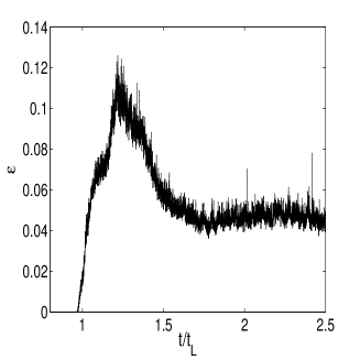
Figure 1: The mean energy dissipation rate $\epsilon$ versus time for $\alpha=2$ (for clarity we show data for $0.8\leq t/t_{L}\leq 2.5$); these data have been averaged over 2000 initial conditions. The main peak at $t/t_{L}\simeq 1.2$ is a signature of cascade completion. For $\alpha=0$ $\epsilon$ displays a similar peak.

Figure 2: (a) Log-log plot of the kinetic energy spectrum $E(k_{n})=S_{2}(k_{n})/k_{n}$ versus $k_{n}$ with the period-three oscillations (see text). The black dashed line corresponds to the K41 scaling prediction $E(k_{n})\sim k^{-5/3}$. (b) Log-log plot of $\Sigma_{2}(k_{n})/k_{n}$ versus $k_{n}$; note that the period-three oscillations are suppressed here; the black dashed line indicates the K41 scaling prediction.

Our results for the equal-time exponents $\zeta_{p}$ for $\alpha=0$ and $\alpha=2$ are presented in Table 1. By comparing Columns $2$ and $3$ in this Table we see that the exponents for both values of $\alpha$ agree with each other and with the exponents reported earlier for statistically steady turbulence [4]. Thus we reconfirm the universality of equal-time exponents: they neither depend on the precise dissipation mechanism nor on whether we consider statistically steady or decaying turbulence.

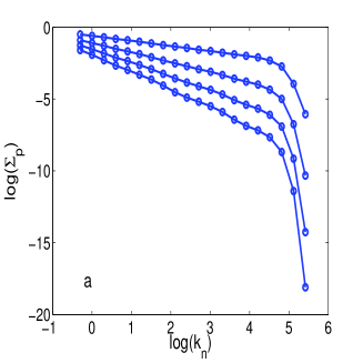
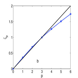
Figure 3: (a) Log-log plot of the modified structure function $\Sigma_{p}$, for $p=1$ to $4$ (top to bottom), versus $k_{n}$ for $\alpha=2$ and number of shells $N=35$ (we show data only for the first $22$ shells). (b) Plot of the equal-time multiscaling exponents $\zeta_{p}$ (obtained from (a) and listed in Table 1) versus the order $p$. The open circles (o), connected by a curve to guide the eye, indicate data from our numerical simulations; the thick black line is the K41 prediction $\zeta_{p}^{K41}=p/3$.

Table 1: Our results for the equal-time multiscaling exponents $\zeta_{p}$ at cascade completion for $\alpha=0$ (Column 2) and $\alpha=2$ (Column 3). We indicate, in parentheses, the ranges of shell numbers $n$ over which we fit our data for equal-time structure functions to obtain these exponents. Note that the exponents in Columns 2 and 3 agree very well with each other.

order-$p$	$\zeta_{p}$ (4-14)	$\zeta_{p}$ (4-16)
1	0.380 $\pm$ 0.001	0.37 $\pm$ 0.01
2	0.709 $\pm$ 0.003	0.699 $\pm$ 0.008
3	1.000 $\pm$ 0.005	1.003 $\pm$ 0.008
4	1.266 $\pm$ 0.008	1.29 $\pm$ 0.02
5	1.51 $\pm$ 0.01	1.55 $\pm$ 0.03
6	1.74 $\pm$ 0.02	1.79 $\pm$ 0.05

In Ref. [4] the dynamic-multiscaling exponents $z^{I}_{p,M}$ and $z^{D}_{p,M}$ were obtained, by using integral- and derivative-time scales, for statistically steady turbulence in the GOY model with $\alpha=0$. We give below an overview of our recent results for dynamic multiscaling but for decaying turbulence; for a detailed discussion of these results we refer the reader to Ref. [23].

Time-dependent structure functions in decaying turbulence must, of course, depend on the origin of time $t_{0}$ from which we start making measurements. It turns out that this dependence can be eliminated by normalising these structure functions by their values at the origin of time; we have shown this analytically for the Kraichnan model [28, 29] for passive-scalar turbulence and numerically in several other models [23]. We present some representative numerical results for the GOY model below for which we use the normalised time-dependent structure functions

$$Q_{p}(k_{n},t)=\frac{F_{p}(k_{n},t_{0},t)}{F_{p}(k_{n},t_{0},0)}.$$ (18)

It turns out that $Q_{p}$ does not depend on $t_{0}$ as shown explicitly in Figure 4 for $p=4$ and $n=5$. This is why we have not displayed $t_{0}$ as an argument of $Q_{p}$.

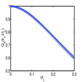
Figure 4: Plots of $Q_{4}(k_{n},t/t_{L})$ for $n=5$ obtained from 6 different values of $t_{0}$; successive values of $t_{0}$ are separated by 0.5$t_{L}$. Since the symbols used for different values of $t_{0}$ are indistinguishable on the scale of this figure, we conclude that $Q_{4}$ does not depend on $t_{0}$.

Given that $Q_{p}$ does not depend on $t_{0}$, we can use expressions such as (9-10), with ${\cal F}_{p}$ replaced by $Q_{p}$, to obtain dynamic-multiscaling exponents for decaying turbulence. We consider here the order-1 integral- and order-2 derivative-time scales and the associated exponents $z^{I}_{p,1}$ and $z^{D}_{p,2}$, respectively.

To calculate the integral-time scale $T^{I}_{p,1}$, we evaluate the integral in equation (7) with $Q_{p}$ instead of ${\cal F}_{p}$ and the upper limit replaced by $t_{\mu}$, the time at which $Q_{p}(k_{n},t)$ reaches a value $\mu\in[0,1]$. We should, of course, use $\mu=0$, i.e., $t_{\mu}=\infty$, but it is hard to obtain well-averaged data for large $t$, so we use $\mu=0.6$. We have checked that our results are not affected significantly if we restrict ourselves to the range $0.4\leq\mu\leq 0.7$. In Figure 5(a) we show representative plots of $Q_{4}$ versus time $t/t_{L}$ for shells $n=3,4,7,$ and $9$ and $\alpha=2$; from this we obtain $T^{I}_{4,1}$ as described above. The slopes of log-log plots of $T^{I}_{p,1}$ versus $k_{n}$ now yield $z^{I}_{p,1}$ as shown in Figure 5(b) for $p=4$. The derivative-time scale $T^{D}_{p,2}$ is calculated by using a sixth-order, centred difference scheme. The derivative-time exponent $z^{D}_{p,2}$ is then obtained from slopes of log-log plots of $T^{D}_{p,2}$ versus $k_{n}$.

Tables 2 and 3 summarise our results for the dynamic-multiscaling exponents. All these exponents have been calculated for $k_{n}$ in the inertial range $4\leq n\leq 14$; the exponents $z^{D}_{p,2}$ are shown only for $\alpha=0$. In Tables 2 and 3 we also give the exponents that we get by using the bridge relations (11) and (12) along with the equal-time exponents given in Table 1; there is good agreement between the exponents from our numerical simulations and those obtained via the bridge relations. Moreover, the exponents $z^{I}_{p,1}$ and $z^{D}_{p,2}$, for $\alpha=0$, and $z^{I}_{p,1}$, for $\alpha=2$, which we obtain for decaying turbulence, are equal (within error bars) to their counterparts (see Table 2 of Ref. [4]) for statistically steady turbulence. Thus the dynamic-multiscaling exponents for the GOY model are universal. Plots of these exponents versus $p$ are shown in Figures 6(a) and 6(b).

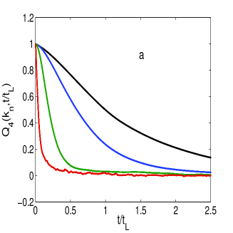
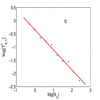
Figure 5: (a) Illustrative plots of the normalised, fourth-order, time-dependent structure function $Q_{4}(k_{n},t)$ versus time $t/t_{L}$ for shells $n=3,4,7$ and $9$ (from top to bottom). (b) A log-log plot of the integral-time scale $T^{I}_{4,1}$ versus $k_{n}$; the integral-time exponent $z_{4,1}^{I}=0.728\pm 0.006$ follows from the slope of the line (in the range $4\leq n\leq 12$).

Table 2: Column 2: The dynamic multiscaling exponents $z^{I}_{p,1}$ from the bridge relation (11) and our numerical results for $\zeta_{p}$ (Table 1). Column 3: The same exponents as in Column 2 but now obtained from our numerical simulations of decaying turbulence in the GOY shell model (for the case $\alpha=2$). Note the agreement between the exponents in Columns 2 and 3.

order-$p$	$z^{I}_{p,1}$[Eq.(11)]	$z^{I}_{p,1}$
1	0.630 $\pm$ 0.001	0.62 $\pm$ 0.01
2	0.675 $\pm$ 0.009	0.683 $\pm$ 0.003
3	0.69 $\pm$ 0.01	0.712 $\pm$ 0.004
4	0.71 $\pm$ 0.02	0.728 $\pm$ 0.006
5	0.74 $\pm$ 0.05	0.750 $\pm$ 0.009
6	0.76 $\pm$ 0.08	0.76 $\pm$ 0.01

Table 3: Dynamic multiscaling exponents from our simulations of decaying turbulence in the GOY model with $\alpha=0$: The bridge relations (11-12) are used along with the equal-time exponents $\zeta_{p}$ for $\alpha=0$ (Table 1) to calculate $z^{I}_{p,1}$ (Column 2) and $z^{D}_{p,2}$ (Column 4). The corresponding dynamic-multiscaling exponents that we obtain from our numerical study of the normalised, time-dependent structure functions $Q_{p}$ are given in Columns 3 and 5.

order-$p$	$z^{I}_{p,1}$[Eq.(11)]	$z^{I}_{p,1}$	$z^{D}_{p,2}[Eq.(\ref{zdpm})]$	$z^{D}_{p,2}$
1	0.620 $\pm$ 0.001	0.60 $\pm$ 0.02	0.690 $\pm$ 0.006	0.687 $\pm$ 0.003
2	0.671 $\pm$ 0.004	0.67 $\pm$ 0.03	0.72 $\pm$ 0.01	0.719 $\pm$ 0.005
3	0.709 $\pm$ 0.008	0.707 $\pm$ 0.006	0.74 $\pm$ 0.02	0.743 $\pm$ 0.007
4	0.73 $\pm$ 0.01	0.736 $\pm$ 0.008	0.76 $\pm$ 0.03	0.75 $\pm$ 0.01
5	0.75 $\pm$ 0.02	0.752 $\pm$ 0.009	0.77 $\pm$ 0.03	0.77 $\pm$ 0.02
6	0.77 $\pm$ 0.03	0.76 $\pm$ 0.02	0.77 $\pm$ 0.03	0.76 $\pm$ 0.02

The universality of dynamic exponents also goes through for models of passive-scalar turbulence as we show in Refs. [5, 23]. It turns out that the Kraichnan model [28, 29] shows simple scaling. However, a shell-model version of a passive scalar advected by GOY-model velocities exhibits dynamic multiscaling with dynamic exponents that depend on the degree $M$, defined in equations (7-8), but not on the order $p$.

We hope our detailed numerical simulations of dynamic multiscaling in the GOY shell model for fluid turbulence will lead to experiments designed to measure time-dependent Lagrangian or quasi-Lagrangian structure functions in fluid turbulence. Advances in experimental techniques have made it possible to get good data for, say, the acceleration of Lagrangian particles [30]. We believe such techniques can be refined to measure the sorts of time-dependent structure functions we have discussed here.

We would like to thank Prasad Perlekar and Ganapati Sahoo for discussions, UGC and DST (India) for support, and SERC (IISc) for computational resources. One of us (RP) is also part of the International Collaboration for Turbulence Research (ICTR).

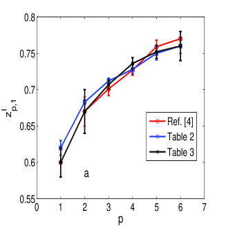
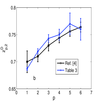
Figure 6: Plots of the dynamic multiscaling exponents (a) $z^{I}_{p,1}$ and (b) $z^{D}_{p,2}$ versus $p$; the error bars are obtained as described in the text. These plots compare data for statistically steady turbulence in the GOY model (from Table 2 in Ref. [4]) and our data for decaying turbulence in the GOY model with normal viscosity ($\alpha=0$) and hyperviscosity ($\alpha=2$); and they illustrate the universality of dynamic-multiscaling exponents that we discus in the text.

References

- [1] U. Frisch, Turbulence: The Legacy of A.N. Kolmogorov (Cambridge University, Cambridge, England, 1996).
- [2] P.M. Chaikin and T.C. Lubensky, Principles of Condensed Matter Physics (Cambridge University, Cambridge, England, 2004).
- [3] V.S. L’vov, E. Podivilov, and I. Procaccia, Phys. Rev. E 55,7030 (1997).
- [4] D. Mitra and R. Pandit, Phys. Rev. Lett. 93, 2 (2004).
- [5] D. Mitra and R. Pandit, Phys. Rev. Lett. 95, 144501 (2005).
- [6] V.I. Belinicher and V.S. L’vov, Sov. Phys. JETP 66, 303(1987).
- [7] Y. Kaneda, T. Ishihara, and K. Gotoh, Phys. Fluids 11, 2154 (1999).
- [8] F. Hayot and C. Jayaprakash, Phys. Rev. E 57, R4867 (1998).
- [9] F. Hayot and C. Jayaprakash, Int. J. Mod. Phys. B 14, 1781 (2000).
- [10] E. Gledzer, Sov. Phys. Dokl. 18, 216 (1973).
- [11] K. Ohkitani and M. Yamada, Prog. Theor. Phys. 81, 329 (1989).
- [12] P.C. Hohenberg and B.I. Halperin, Rev. Mod. Phys. 49, 435 (2004) and references therein.
- [13] A.N. Kolmogorov, Dokl. Akad. Nauk SSSR 30, 301 (1941).
- [14] A.N. Kolmogorov, Dokl. Akad. Nauk SSSR 31, 538 (1941).
- [15] E. Leveque and Z.S. She, Phys. Rev. Lett 75, 2690 (1995).
- [16] N. Schorghofer, L. Kadanoff, and D. Lohse, Physica D 88, 40 (1995).
- [17] P. Ditlevsen, Phys. Fluids 9, 1482 (1997).
- [18] V. Borue and S.A. Orzsag, Phys. Rev. E 51, R856(1995).
- [19] V. S. L’vov, I. Procaccia, and D. Vandembroucq, Phys. Rev. Lett 81, 802 (1998).
- [20] V.S. L’vov, R.A. Pasmanter, A. Pomyalov, and I. Procaccia, Phys. Rev. E 67, 066310 (2003).
- [21] S.B. Pope, Turbulent Flows (Cambridge University, Cambridge, England, 2000).
- [22] V. S. L’vov and V. L. Lebedev, Phys. Rev. E 47, 1794 (1993).
- [23] S. S. Ray, D. Mitra, and R. Pandit, to be published.
- [24] S. K. Dhar, A. Sain, and R. Pandit, Phys. Rev. Lett. 78, 2964 (1997).
- [25] D. Pisarenko, L. Biferale, D. Courvoisier, U. Frisch, and M. Vergassola, Phys. Fluids A 5, 2533 (1993).
- [26] G. Sahoo, D. Mitra, and R. Pandit, to be published.
- [27] L. Kadanoff, D. Lohse, J. Wang, and R. Benzi, Phys. Fluids 7, 617 (1995).
- [28] R. Kraichnan, Phys. Fluids 11, 945 (1968).
- [29] G. Falkovich, K. Gawedzki and M. Vergassola, Rev. Mod. Phys. 73, 913 (2001).
- [30] A. La Porta, G.A. Voth, A.M. Crawford, J. Alexander, and E. Bodenschatz Nature 409, 1017 (2001).