Deeply Virtual Neutrino Scattering

Abstract

We investigate the extension of the deeply virtual Compton scattering process into the weak interaction sector.

PACS number(s): 13.15.+g, 13.40.-f, 13.40.Gp, 13.60.-r, 13.60.Fz

I Introduction

Standard electromagnetic Compton scattering provides a unique tool for studying hadrons, which is one of the most fascinating frontiers of modern science. In this process the relevant Compton scattering amplitude probes the hadron structure by means of two quark electromagnetic currents. We argue that replacing one of the currents with the weak interaction current can promise a new insight.

The paper is organized as follows. In Sec. II we briefly discuss the features of the handbag factorization scheme. We introduce a new set of phenomenological functions, known as generalized parton distributions (GPDs) Muller:1998fv ; Ji:1996ek ; Ji:1996nm ; Radyushkin:1996nd ; Radyushkin:1996ru ; Radyushkin:1997ki , and discuss some of their basic properties in Sec. III. An application of the GPD formalism to the neutrino-induced deeply virtual Compton scattering in the kinematics relevant to future high-intensity neutrino experiments is given in Sec. IV. The cross section results are presented in Sec. V. Finally, in Sec. VI we draw some conclusions and discuss future prospects.

Some of the formal results in this paper have appeared in preliminary reports in Refs. Psaker:2004sf and Psaker:2005wj , whereas a comprehensive analysis of the weak neutral and weak charged current DVCS reactions in collaboration with W. Melnitchouk and A. Radyushkin has been presented in Ref. Psaker:2006gj . Neutrino scattering off nucleons for neutral and charged currents was also discussed in Refs. Amore:2004ng and Coriano:2004bk , respectively.

II Handbag Factorization

The underlying theory of strong interaction physics is the universally accepted nonAbelian gauge field theory known as quantum chromodynamics (QCD). The theory postulates that hadrons are composite objects made up of quarks, and that the color interaction between them is mediated by gluons as the gauge bosons. In principle, QCD embraces all phenomena of hadronic physics, in other words, the fundamental building blocks of hadrons (i.e. quarks and gluons) are known, and further the interactions between them are described by the well-established QCD Lagrangian. Nevertheless, knowing the first principles is not sufficient. The main difficulty is that QCD is formulated in terms of colored degrees-of-freedom, while the physical hadrons observed in the experiments are colorless. How to translate the information obtained from the experiments at the hadronic level into the language of quark and gluon fields has yet to be answered, and it represents a challenging task.

One way to tackle this problem is to consider projecting these fields onto the hadronic states, and then use different phenomenological functions (e.g. form factors, parton distribution functions (PDFs), distribution amplitudes and GPDs) to describe the resulting hadronic matrix elements. The key idea of this approach is the handbag factorization. According to this property, in the specific kinematical regime featuring the presence of a large invariant, such as the virtuality of the probe or the momentum transfer, the amplitude of the process splits into the hard (short-distance) part with only one active parton propagating along the light-cone and the soft (long-distance) part represented by the lower blob, see Fig. 1. The asymptotically free nature of QCD allows us to compute the short-distance interactions by means of perturbation theory, whereas the nonperturbative stages of interactions are expressed in terms of well-defined quark-gluon operators taken on the light-cone, and being sandwiched between the hadronic states. These matrix elements, which accumulate the information about the long-distance dynamics of the process, are process independent nonperturbative objects. Thus they are parametrized in terms of universal phenomenological functions, and they can be measured with the help of different probes (e.g. photons and weak interaction bosons).

There are several situations, where the handbag contribution plays an essential role:

• Both initial and final photons are highly virtual and have equal space-like virtualities. This situation corresponds to the forward virtual Compton scattering amplitude. Its imaginary part, through the optical theorem, determines the structure functions of deeply inelastic lepton scattering (DIS).

• The condition on photon virtualities may be relaxed in a sense that the initial photon is still far off-shell but the final photon is real and the invariant momentum transfer to the hadron is small. The situation corresponds to the nonforward virtual Compton scattering amplitude, which is accessible through processes such as deeply virtual Compton scattering (DVCS) and deeply virtual meson production.

• The configuration, in which both photons in the initial and final states are real but the invariant momentum transfer is large. The physical process corresponding to this situation is known as wide-angle real Compton scattering.

Figure 1: Handbag diagram. In the lowest QCD approximation, both photons couple to the same quark line through point-like vertices.

III Generalized Parton Distributions

The description of specific aspects of the hadron structure is provided by several different phenomenological functions. The well-known examples are the so-called old phenomenological functions such as form factors, PDFs and distribution amplitudes since they have been around for a long time. On the other hand, the concept of GPDs is new. These new functions, as hybrids of the old ones, provide the most complete information about the hadron structure. In fact, the old phenomenological functions are just the limiting case of GPDs. Like PDFs, GPDs encapsulate longitudinal momentum distributions of hadron’s constituents, however, at the same time, like form factors, they also provide the information about their transverse coordinate distributions, and hence give a comprehensive three-dimensional snapshot of the substructure of the hadron. Moreover, the universality of GPDs enables one to develop a unified description of wide variety of different hard (i.e. light-cone dominated) processes, both inclusive and exclusive.

In the symmetric partonic picture, see Fig. 2, we treat both the initial and final hadron momenta symmetrically by introducing the average hadron momentum $p\equiv\left(p_{1}+p_{2}\right)/2$. Here $x$ is the usual light-cone momentum fraction. In addition, another scaling variable is introduced, the so- called skewness $\xi$. It is defined as the coefficient of the proportionality between the light-cone plus components of the momentum transfer, $r\equiv p_{1}-p_{2}$, and average hadron momentum, $\xi\equiv r^{+}/2p^{+}$, and it specifies the longitudinal momentum asymmetry. Clearly, in the skewed (nonforward) kinematics GPDs uncover much richer information about the hadron structure, which is not accessible in DIS, or in general in any inclusive process. By removing the parton with the light-cone momentum fraction $x+\xi$ from the hadron, and replacing it at some later point on the light-cone with the parton of fraction $x-\xi$, GPDs measure the coherence between the two parton momentum states in the hadron as well as their spin correlations. Finally, by considering two different hadrons in the initial and final states one can study flavor nondiagonal GPDs, for example, in the proton-to-neutron transition accessible through the exclusive charged pion electroproduction, the proton-to-$\Lambda$ transition in the kaon electroproduction or the nucleon-to-$\Delta$ transition.

Figure 2: Symmetric partonic picture.

Since $-1\leq x\leq 1$, the momentum fractions $x\pm\xi$ of the active partons can be either positive or negative, and for that reason GPDs have three distinct regions. When $\xi\leq x\leq 1$ both partons represent quarks, while for $-1\leq x\leq-\xi$ they are both antiquarks. In these two regions GPDs are just a generalization of PDFs. In the central region, $-\xi\leq x\leq\xi$, which is often referred to as the mesonic region, the partons represent the quark-antiquark pair. Here GPDs behave like meson distribution amplitudes.

At the leading twist-2 level, the hadron structure information can be parametrized in terms of two unpolarized and two polarized GPDs denoted by $H$, $E$ and $\widetilde{H}$, $\widetilde{E}$, respectively. They are functions of three variables $\left(x,\xi,t\right)$, where $t=r^{2}$ is the invatiant momentum transfer, and further they are defined for each quark flavor $f$. GPDs have interesting properties linking them to PDFs and form factors. In the forward limit, $p_{1}=p_{2}$, $r=0$, $\xi=0$, $t=0$, they reduce to PDFs. In particular, $H_{f}$ and $\widetilde{H}_{f}$ coincide with the quark density distribution $f_{N}\left(x\right)$ and the quark helicity distribution $\Delta f_{N}\left(x\right)$. We write the so-called reduction formulas,

$$H_{f}\left(x,0,0\right)=\left\{\begin{array}[]{cc}f_{N}\left(x\right)&x>0\\ -\bar{f}_{N}\left(-x\right)&x<0\\ \end{array}\right.$$ (1)

and

$$\widetilde{H}_{f}\left(x,0,0\right)=\left\{\begin{array}[]{cc}\Delta f_{N}\left(x\right)&x>0\\ \Delta\bar{f}_{N}\left(-x\right)&x<0,\\ \end{array}\right.$$ (2)

while $E_{f}$ and $\widetilde{E}_{f}$ have no connections to PDFs. They are always accompanied with the momentum transfer, and hence simply not visible in DIS. Even though they have no analogue in the forward limit their limits do exist. In the local limit GPDs reduce to the standard nucleon elastic form factors (i.e. Dirac, Pauli, axial and pseudoscalar form factors),

$$\int_{-1}^{1}dx\;H_{f}\left(x,\xi,t\right)=F_{1f}\left(t\right) \int_{-1}^{1}dx\;E_{f}\left(x,\xi,t\right)=F_{2f}\left(t\right),$$ , (3)

$$\int_{-1}^{1}dx\;\widetilde{H}_{f}\left(x,\xi,t\right)=g_{Af}\left(t\right) \int_{-1}^{1}dx\;\widetilde{E}_{f}\left(x,\xi,t\right)=g_{Pf}\left(t\right).$$ , (4)

We call these relations the sum rules.

GPDs in general are also relevant for the hadron spin structure. In terms of GPDs their second moments at $t=0$ give the quark total angular momentum,

$$J_{q} = \frac{1}{2}\sum_{f}\int_{-1}^{1}dx\;x\left[H_{f}\left(x,\xi,t=0\right)+E_{f}\left(x,\xi,t=0\right)\right].$$ (5)

On the other hand, by decomposing $J_{q}$ into the quark intrinsic spin $\Delta\Sigma$ (measured through polarized DIS) and quark orbital angular momentum $L_{q}$, $J_{q}=\Delta\Sigma/2+L_{q}$, we can access $L_{q}$. Finally, since the total nucleon spin comes from quarks and gluons, $1/2=J_{q}+J_{g}$, we can extract the total angular momentum $J_{g}$ carried by gluons.

IV Deeply Virtual Neutrino Scattering

In recent years, significant effort was made to study GPDs through measurements of hard exclusive electroproduction processes. The simplest process in this respect is the standard electromagnetic DVCS process. Complementary to DVCS different combinations of quark flavors can be accessed by utilizing the weak interaction current in neutrino-induced DVCS (or, alternatively deeply virtual neutrino scattering - DVNS), namely

$$\nu\left(k\right)N\left(p_{1}\right) \longrightarrow e^{-}\left(k^{\prime}\right)N^{\prime}\left(p_{2}\right)\gamma\left(q_{2}\right)$$ (6)

for the charged current, and

$$\nu\left(k\right)N\left(p_{1}\right) \longrightarrow \nu\left(k^{\prime}\right)N\left(p_{2}\right)\gamma\left(q_{2}\right)$$ (7)

for neutral current reactions. The presence of the axial part of the $V-A$ interaction enables to probe a different set of GPDs, i.e. the charge conjugation odd combinations of GPDs as well as charge conjugation even combinations and hence independently measure both the valence and sea content of GPDs. Furthermore, one deals with a different flavor decomposition, in particular, less enhancement from $u$-quarks. An additional feature of the DVNS process is the study of GPDs that are not diagonal in quark flavors, such as those associated with the neutron-to-proton transition.

In the most general case, there are three relevant diagrams for a DVCS-like process, see Fig. 3. The nucleon blob with the boson leg, which can be either a virtual photon or weak interaction boson, and photon leg represents the virtual Compton scattering amplitude. This diagram is referred to as the DVCS diagram or the Compton contribution. The real photon can also be emitted by a lepton as depicted in the remaining two diagrams. They illustrate the Bethe-Heitler process, where the lower blob with one boson leg stands for the electroweak form factor, while the upper part in each diagram can be exactly calculable in QED.

Figure 3: DVCS (a) and Bethe-Heitler (b and c) diagrams contributing to the leptoproduction of a real photon.

In the Bjorken regime, in which the virtuality of the weak boson $-q^{2}_{1}$ and the invariant mass of the weak boson-nucleon system, $s\equiv\left(p_{1}+q_{1}\right)^{2}$, are both sufficiently large while the Bjorken ratio $x_{B}\equiv-q_{1}^{2}/\left[2\left(p_{1}\cdot q_{1}\right)\right]$ is kept finite, the behavior of the virtual Compton scattering amplitude is dominated by the light-like distances. The dominant light-cone singularities are represented by two ($s$- and $u$-channel) handbag diagrams, see Fig. 4, in which the hard quark propagator is convoluted with GPDs. In addition, by keeping the invariant momentum transfer to the nucleon as small as possible we arrive at the so-called DVCS kinematics, $s>-q_{1}^{2}\gg-t$. Accordingly, the $t$-dependence enters only in the soft part of the amplitude.

Figure 4: The $s$- and $u$-channel handbag diagrams for the virtual Compton scattering amplitude.

In our case in terms of symmetric momentum variables, $p\equiv\left(p_{1}+p_{2}\right)/2$ and $q\equiv\left(q_{1}+q_{2}\right)/2$, the virtual Compton scattering amplitude is given by the Fourier transform of the correlation function of the electromagnetic and weak (neutral or charged) interaction currents,

$$\mathsf{\mathcal{T}}_{W}^{\mu\nu} = i\int d^{4}z\;e^{iq\cdot z}\left\langle N^{\prime}\left(p-r/2,s_{2}\right)\right|T\left\{J_{EM}^{\mu}\left(z/2\right)J_{W}^{\nu}\left(-z/2\right)\right\}\left|N\left(p+r/2,s_{1}\right)\right\rangle\ .$$ (8)

The weak current couples to the quark current through two types of vertices, $qqZ^{0}$ and $qqW^{\pm}$, and hence the quark fields at coordinates $\pm z$ can either have the same or different flavor quantum numbers. For that reason, we treat these two cases separately. The method employed to study the amplitude (8) in the DVCS kinematics is based on the nonlocal light-cone expansion of the time-ordered product of currents in terms of QCD bilocal operators in coordinate space Balitsky:1987bk ,

$$iT\left\{J_{EM}^{\mu}\left(z/2\right)J_{WN}^{\nu}\left(-z/2\right)\right\} = -\frac{z_{\rho}}{4\pi^{2}z^{4}}\sum_{f}Q_{f}\left\{c_{V}^{f}\left[s^{\mu\rho\nu\eta}\mathcal{O}_{\eta}^{f-}\left(z\left|0\right.\right)-i\epsilon^{\mu\rho\nu\eta}\mathcal{O}_{5\eta}^{f+}\left(z\left|0\right.\right)\right]\right.$$ (9)

$$\left.-\ c_{A}^{f}\left[s^{\mu\rho\nu\eta}\mathcal{O}_{5\eta}^{f-}\left(z\left|0\right.\right)-i\epsilon^{\mu\rho\nu\eta}\mathcal{O}_{\eta}^{f+}\left(z\left|0\right.\right)\right]\right\}\ ,$$

where $Q_{f}$ denotes the electric charge of the quark with flavor $f$ (in units of $\left|e\right|$), $c_{V}^{f}$ and $c_{A}^{f}$ are the corresponding weak vector and axial vector charges, $s^{\mu\rho\nu\eta}\equiv g^{\mu\rho}g^{\nu\eta}+g^{\mu\eta}g^{\rho\nu}-g^{\mu\nu}g^{\rho\eta}$ is the symmetric tensor and $\epsilon^{\mu\rho\nu\eta}$ the antisymmetric tensor in Lorentz indices ($\mu,\nu$), and further

$$\mathcal{O}_{\eta}^{f\pm}\left(z\left|0\right.\right) \equiv \left[\bar{\psi}_{f}\left(z/2\right)\gamma_{\eta}\psi_{f}\left(-z/2\right)\pm\left(z\rightarrow-z\right)\right]\ ,$$ (10)

$$\mathcal{O}_{5\eta}^{f\pm}\left(z\left|0\right.\right) \equiv \left[\bar{\psi}_{f}\left(z/2\right)\gamma_{\eta}\gamma_{5}\psi_{f}\left(-z/2\right)\pm\left(z\rightarrow-z\right)\right]\ ,$$ (11)

are the vector and axial vector bilocal operators, respectively. Unlike the weak neutral current sector explicily presented here, the expansion for the weak charged and electromagnetic currents is a bit more complicated due to the fact that $W^{\pm}$ carries an electric charge. Thus we end up with different nucleons in the initial and final states and accordingly, the bilocal operators are accompanied with different electric charges as well as flavors.

Next we isolate the twist-2 part of these operators, and sandwich it between the initial and final nucleon states. To construct the parametrization for nonforward matrix elements on the light-cone, we use a spectral representation in terms of eight GPDs, which have well-defined symmetry properties with respect to $x$. In particular, in case of the weak neutral current we have

$$\left\langle N\left(p_{2},s_{2}\right)\right|\mathcal{O}^{f\pm}\left(z\left|0\right.\right)\left|N\left(p_{1},s_{1}\right)\right\rangle_{z^{2}=0} = \bar{u}\left(p_{2},s_{2}\right)\not\!zu\left(p_{1},s_{1}\right)\int_{-1}^{1}dx\;e^{ixp\cdot z}H_{f}^{\pm}\left(x,\xi,t\right)$$ (12)

$$+\bar{u}\left(p_{2},s_{2}\right)\frac{\left(\not\!z\not\!r-\not\!r\not\!z\right)}{4M}u\left(p_{1},s_{1}\right)\int_{-1}^{1}dx\;e^{ixp\cdot z}E_{f}^{\pm}\left(x,\xi,t\right)\ ,$$

$$\left\langle N\left(p_{2},s_{2}\right)\right|\mathcal{O}_{5}^{f\pm}\left(z\left|0\right.\right)\left|N\left(p_{1},s_{1}\right)\right\rangle_{z^{2}=0} = \bar{u}\left(p_{2},s_{2}\right)\not\!z\gamma_{5}u\left(p_{1},s_{1}\right)\int_{-1}^{1}dx\;e^{ixp\cdot z}\widetilde{H}_{f}^{\mp}\left(x,\xi,t\right)$$ (13)

$$-\bar{u}\left(p_{2},s_{2}\right)\frac{\left(r\cdot z\right)}{2M}\gamma_{5}u\left(p_{1},s_{1}\right)\int_{-1}^{1}dx\;e^{ixp\cdot z}\widetilde{E}_{f}^{\mp}\left(x,\xi,t\right)\ .$$

In contrast to the electromagnetic DVCS process, which measures only the plus GPDs (i.e. the sum of quark and antiquark distributions), the DVNS process gives also access to the minus distributions (i.e. the valence configuration) associated with the axial part of the $V-A$ interaction. Moreover, it’s important to note that since the matrix elements with the weak charged interaction current involve different flavor combinations the corresponding GPDs, which parametrize these matrix elements, are nondiagonal in quark flavor.

The final expression for the weak neutral leading twist-2 Compton scattering amplitude reads

$$\mathcal{T}_{WN}^{\mu\nu} = -\frac{1}{4\left(p\cdot q\right)}\left\{\left[\frac{1}{\left(p\cdot q_{2}\right)}\left(p^{\mu}q_{2}^{\nu}+p^{\nu}q_{2}^{\mu}\right)-g^{\mu\nu}\right]\right.$$ (14)

$$\times\left[\mathcal{H}_{WN}^{+}\left(\xi,t\right)\bar{u}\left(p_{2},s_{2}\right)\not\!q_{2}u\left(p_{1},s_{1}\right)+\mathcal{E}_{WN}^{+}\left(\xi,t\right)\bar{u}\left(p_{2},s_{2}\right)\frac{\left(\not\!q_{2}\not\!r-\not\!r\not\!q_{2}\right)}{4M}u\left(p_{1},s_{1}\right)\right.$$

$$\hskip 14.22636pt\left.-\widetilde{\mathcal{H}}_{WN}^{-}\left(\xi,t\right)\bar{u}\left(p_{2},s_{2}\right)\not\!q_{2}\gamma_{5}u\left(p_{1},s_{1}\right)+\widetilde{\mathcal{E}}_{WN}^{-}\left(\xi,t\right)\frac{\left(q_{2}\cdot r\right)}{2M}\bar{u}\left(p_{2},s_{2}\right)\gamma_{5}u\left(p_{1},s_{1}\right)\right]$$

$$+\left[\frac{1}{\left(p\cdot q_{2}\right)}i\epsilon^{\mu\nu\rho\eta}q_{2\rho}p_{\eta}\right]$$

$$\times\left[\widetilde{\mathcal{H}}_{WN}^{+}\left(\xi,t\right)\bar{u}\left(p_{2},s_{2}\right)\not\!q_{2}\gamma_{5}u\left(p_{1},s_{1}\right)-\widetilde{\mathcal{E}}_{WN}^{+}\left(\xi,t\right)\frac{\left(q_{2}\cdot r\right)}{2M}\bar{u}\left(p_{2},s_{2}\right)\gamma_{5}u\left(p_{1},s_{1}\right)\right.$$

$$\hskip 14.22636pt\left.\left.-\mathcal{H}_{WN}^{\mathit{-}}\left(\xi,t\right)\bar{u}\left(p_{2},s_{2}\right)\not\!q_{2}u\left(p_{1},s_{1}\right)-\mathcal{E}_{WN}^{\mathit{-}}\left(\xi,t\right)\bar{u}\left(p_{2},s_{2}\right)\frac{\left(\not\!q_{2}\not\!r-\not\!r\not\!q_{2}\right)}{4M}u\left(p_{1},s_{1}\right)\right]\right\}\ ,$$

where

$$\mathcal{H}_{WN}^{+\left(-\right)}\left(\xi,t\right) \equiv \sum_{f}Q_{f}c_{V\left(A\right)}^{f}\int_{-1}^{1}\frac{dx}{\left(x-\xi+i0\right)}H_{f}^{+\left(-\right)}\left(x,\xi,t\right)$$ (15)

$$= \sum_{f}Q_{f}c_{V\left(A\right)}^{f}\int_{-1}^{1}dx\;H_{f}\left(x,\xi,t\right)\left(\frac{1}{x-\xi+i0}\pm\frac{1}{x+\xi}\right)\;,$$

$$\mathcal{E}_{WN}^{+\left(-\right)}\left(\xi,t\right) \equiv \sum_{f}Q_{f}c_{V\left(A\right)}^{f}\int_{-1}^{1}\frac{dx}{\left(x-\xi+i0\right)}E_{f}^{+\left(-\right)}\left(x,\xi,t\right)$$ (16)

$$= \sum_{f}Q_{f}c_{V\left(A\right)}^{f}\int_{-1}^{1}dx\;E_{f}\left(x,\xi,t\right)\left(\frac{1}{x-\xi+i0}\pm\frac{1}{x+\xi}\right)\;,$$

$$\widetilde{\mathcal{H}}_{WN}^{+\left(-\right)}\left(\xi,t\right) \equiv \sum_{f}Q_{f}c_{V\left(A\right)}^{f}\int_{-1}^{1}\frac{dx}{\left(x-\xi+i0\right)}\widetilde{H}_{f}^{+\left(-\right)}\left(x,\xi,t\right)$$ (17)

$$= \sum_{f}Q_{f}c_{V\left(A\right)}^{f}\int_{-1}^{1}dx\;\widetilde{H}_{f}\left(x,\xi,t\right)\left(\frac{1}{x-\xi+i0}\mp\frac{1}{x+\xi}\right)\;,$$

$$\widetilde{\mathcal{E}}_{WN}^{+\left(-\right)}\left(\xi,t\right) \equiv \sum_{f}Q_{f}c_{V\left(A\right)}^{f}\int_{-1}^{1}\frac{dx}{\left(x-\xi+i0\right)}\widetilde{E}_{f}^{+\left(-\right)}\left(x,\xi,t\right)$$ (18)

$$= \sum_{f}Q_{f}c_{V\left(A\right)}^{f}\int_{-1}^{1}dx\;\widetilde{E}_{f}\left(x,\xi,t\right)\left(\frac{1}{x-\xi+i0}\mp\frac{1}{x+\xi}\right)\;,$$

are the so-called Compton form factors given by the integrals of GPDs. The amplitude (14) has both real and imaginary parts. The real part is obtained by the principal value prescription, whereas the imaginary part constrains evaluating GPDs at the specific point $x=\pm\xi$.

In the laboratory frame as the target rest frame we choose a coordinate system, in which the weak boson four-momentum has no transverse components, see Fig. 5. The differential cross section is given by

$$\frac{d^{4}\sigma}{dx_{B}dQ_{1}^{2}dtd\varphi} = \frac{1}{32}\frac{1}{\left(2\pi\right)^{4}}\frac{x_{B}y^{2}}{Q_{1}^{4}}\frac{1}{\sqrt{1+4x_{B}^{2}M^{2}/Q_{1}^{2}}}\left|{\textrm{T}}\right|^{2}\,\,,$$ (19)

where the invariant matrix element is the sum of both the Compton and Bethe-Heitler contributions, $\mathrm{T}=\mathrm{T}_{C}+\mathrm{T}_{BH}$. Furthermore, we require the following:

• The energy of the incoming lepton beam is fixed at $\omega=20\;\mathrm{GeV}$.

• The invariant mass squared of the weak boson-nucleon system should be above the resonance region, $s\geq 4\;\mathrm{GeV}^{2}$.

• The virtuality of the incoming boson has to be large enough to ensure light-cone dominance of the scattering process, $Q_{1}^{2}\geq 2.5\;\mathrm{GeV}^{2}$.

• The momentum transfer squared should be as small as possible, e.g. $0.1\;\mathrm{GeV^{2}}\leq\left|t\right|\leq 0.2\;\mathrm{GeV^{2}}$.

We pick one kinematical point, in particular with the parameters $\omega=20\;\mathrm{GeV}$, $Q_{1}^{2}=2.5\;\mathrm{GeV}^{2}$, $x_{B}=0.35$ and $y=0.19$, and plot the invariant momentum transfer as a function of the angle $\theta_{B\gamma}$ between the incoming virtual weak boson and outgoing real photon, see Fig. 6. The values vary from $-0.15\;\mathrm{GeV}^{2}$ at zero degrees up to $-1\;\mathrm{GeV}^{2}$ at $\theta_{B\gamma}=12^{\circ}$. Finally, we set the angle between the two planes to zero. In the so-called in-plane kinematics the polar angles of both incoming and scattered leptons are also fixed to $\phi=20.2^{\circ}$ and $\phi^{\prime}=25.3^{\circ}$, respectively.

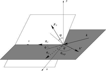
Figure 5: The kinematics of the generalized DVCS process in the target rest frame. The lepton momenta $k$ and $k^{\prime}$ define the lepton scattering plane and the momenta of the final photon and outgoing nucleon define the nucleon scattering plane.

Figure 6: Invariant momentum transfer as a function of the scattering angle between the incoming virtual weak boson and outgoing real photon.

We use a simple model for nucleon GPDs Guichon:1998xv ; Radyushkin:1998rt ; Belitsky:2001ns ; Carlitz:1976in ; Goshtasbpour:1995eh with the following assumptions: the sea quark contribution is neglibile and hence the plus and minus distributions coincide; the $t$-dependence of GPDs, which is driven by the corresponding nucleon form factors, factorizes from the dependence on the other two scaling variables, $x$ and $\xi$; the $\xi$-dependence of GPDs appears only in the $\widetilde{E}_{f}$ distribution.

In the weak neutral case we consider a neutrino-induced DVCS on a proton target through the exchange of $Z^{0}$. There is no Bethe-Heitler contamination (the photon cannot be emitted from the neutrino leg) and for that reason, we measure the pure Compton contribution,

$$\mathrm{T}_{\nu p} = \sqrt{2}\left|e\right|G_{F}\bar{u}\left(k^{\prime}\right)\gamma_{\nu}\left(1-\gamma_{5}\right)u(k)\epsilon_{\mu}^{*}\left(q_{2}\right)\mathcal{T}_{WN}^{\mu\nu}\ .$$ (20)

In the weak charged current sector we examine scattering off neutrinos, which convert into muons by emission of $W^{+}$, on a neutron target. Here in addition to the Compton part,

$$\mathrm{T}_{C\nu n} = \sqrt{2}\left|e\right|G_{F}\bar{u}\left(k^{\prime}\right)\gamma_{\nu}\left(1-\gamma_{5}\right)u\left(k\right)\epsilon_{\mu}^{*}\left(q_{2}\right)\mathcal{T}_{WC}^{\mu\nu}\ ,$$ (21)

the Bethe-Heitler contribution is present,

$$\mathrm{T}_{BH\nu n} = \sqrt{2}\left|e\right|G_{F}\epsilon_{\mu}^{*}\left(q_{2}\right)\bar{u}\left(k^{\prime}\right)\left[\frac{\gamma^{\mu}\left(\not\!k^{\prime}+\not\!q_{2}\right)\gamma^{\nu}\left(1-\gamma_{5}\right)}{\left(k^{\prime}+q_{2}\right)^{2}}\right]u\left(k\right)\left\langle p\left(p_{2},s_{2}\right)\right|J_{\nu}^{CC}\left(0\right)\left|n\left(p_{1},s_{1}\right)\right\rangle\ ,$$ (22)

however, it’s given only by diagram (b) of Fig. 3. Moreover, the isospin symmetry is used to express the nucleon matrix elements that are nondiagonal in quark flavor in terms of flavor diagonal matrix elements Mankiewicz:1997aa .

V Results

We present the cross section results for $\theta_{B\gamma}\leq 12^{\circ}$, which corresponds to taking the invariant momentum transfer $-t<-1\;\mathrm{GeV}^{2}$. The charged current Compton cross section is larger than for the neutral current interaction, see Fig. 7. We compare the magnitude of the Compton contribution relative to the corresponding Bethe-Heitler background by plotting both cross sections together on a logarithmic scale, see Fig. 8. The Compton cross section is significantly larger than the Bethe-Heitler signal. Note also that for the Bethe-Heitler cross section one should expect a pole at the scattering angle $\theta_{B\gamma}=25.3^{\circ}$ when the scattered muon is collinear with outgoing real photon. On the other hand, in the electromagnetic current case the Bethe-Heitler contribution is larger than the Compton for $\theta_{B\gamma}>3^{\circ}$, see Fig. 9. Finally, we plot the ratio of Compton versus Bethe-Heitler cross sections for both weak charged and electromagnetic DVCS. In the forward direction (i.e. for $\theta_{B\gamma}\leq 4^{\circ}$) the Bethe-Heitler cross section is strongly supressed by a factor more than 100 compared to the Compton contribution for the weak charged interaction current, whereas in the electromagnetic current case the ratio between the cross sections remains of order unity, see Fig. 10.

Figure 7: Compton cross sections for the weak neutral DVCS with the neutrino beam (solid line), electron beam (dashed line), and weak charged DVCS with the neutrino beam (dotted line).

Figure 8: Compton (dashed line), Bethe-Heitler (dotted line), magnitude of interference (dashed-dotted line), and total (solid line) cross sections for weak charged DVCS.

Figure 9: As in Fig. 8 but for electromagnetic DVCS.

Figure 10: Ratio of Compton and Bethe-Heitler cross section for weak neutral DVCS with the electron beam (solid line), weak charged DVCS with the neutrino beam (dashed line), and electromagnetic DVCS (dotted line).

VI Summary and Outlook

GPDs provide the most complete and unified description of the internal quark-gluon structure of hadrons, which can be probed through wide variety of both inclusive and exclusive hard processes.

DVNS is an important tool to complement the study of GPDs in the more familiar electro-induced DVCS. In addition to different combinations and flavor decomposition of GPDs, providing a direct measurement of their valence and sea contents, the process enables one to access the distributions that are nondiagonal in quark flavor.

We have computed the twist-2 Compton scattering amplitudes for both weak neutral and weak charged interaction currents by means of the light-cone expansion of the current product in coordinate space. Using a simple model for the nucleon GPDs, which only includes the valence quark contribution, we gave prediction for cross sections in the kinematics relevant to future high-intensity neutrino experiments.

Unlike the standard electromagnetic DVCS process, we find that at small scattering angles the Compton contribution is enhanced relative to the corresponding Bethe-Heitler contribution. Thus a contamination from the Bethe-Heitler background is less of a problem when extracting the weak DVCS signal.

In the future we plan to use more realistic model for nucleon GPDs, which also includes sea quark effects, elaborate separately contributions from the plus and minus distributions, and include the twist-3 terms in order to apply the formalism at moderate energies.

- (1) D. Müller, D. Robaschik, B. Geyer, F. M. Dittes and J. Horejsi, Fortsch. Phys. 42, 101 (1994), hep-ph/9812448.
- (2) X. D. Ji, Phys. Rev. Lett. 78, 610 (1997), hep-ph/9603249.
- (3) X. D. Ji, Phys. Rev. D 55, 7114 (1997), hep-ph/9609381.
- (4) A. V. Radyushkin, Phys. Lett. B 380, 417 (1996), hep-ph/9604317.
- (5) A. V. Radyushkin, Phys. Lett. B 385, 333 (1996), hep-ph/9605431.
- (6) A. V. Radyushkin, Phys. Rev. D 56, 5524 (1997), hep-ph/9704207.
- (7) A. Psaker, hep-ph/0412321.
- (8) A. Psaker, hep-ph/0511283.
- (9) A. Psaker, W. Melnitchouk and A. V. Radyushkin, Phys. Rev. D 75, 054001 (2007), hep-ph/0612269.
- (10) P. Amore, C. Coriano and M. Guzzi, JHEP 0502, 038 (2005), hep-ph/0404121.
- (11) C. Coriano and M. Guzzi, Phys. Rev. D 71, 053002 (2005), hep-ph/0411253.
- (12) I. I. Balitsky and V. M. Braun, Nucl. Phys. B 311, 541 (1989).
- (13) P. A. M. Guichon and M. Vanderhaeghen, Prog. Part. Nucl. Phys. 41, 125 (1998), hep-ph/9806305.
- (14) A. V. Radyushkin, Phys. Rev. D 58, 114008 (1998), hep-ph/9803316.
- (15) A. V. Belitsky, D. Müller and A. Kirchner, Nucl. Phys. B 629, 323 (2002), hep-ph/0112108.
- (16) R. D. Carlitz and J. Kaur, Phys. Rev. Lett. 38, 673 (1977) [Erratum-ibid. 38, 1102 (1977)].
- (17) M. Goshtasbpour and G. P. Ramsey, Phys. Rev. D 55, 1244 (1997), hep-ph/9512250.
- (18) L. Mankiewicz, G. Piller and T. Weigl, Phys. Rev. D 59, 017501 (1999), hep-ph/9712508.