Three-Dimensional Simulations of Inflows Irradiated by a Precessing Accretion Disk in Active Galactic Nuclei: Formation of Outflows

Abstract

We present three-dimensional (3-D) hydrodynamical simulations of gas flows in the vicinity of an active galactic nucleus (AGN) powered by a precessing accretion disk. We consider the effects of the radiation force from such a disk on its environment on a relatively large scale (up to $\sim 10$ pc). We implicitly include the precessing disk by forcing the disk radiation field to precess around a symmetry axis with a given period ($P$) and a tilt angle ($\Theta$). We study time evolution of the flows irradiated by the disk, and investigate basic dependencies of the flow morphology, mass flux, angular momentum on different combinations of $\Theta$ and $P$. As this is our first attempt to model such 3-D gas flows, we consider a simplest form of radiation force i.e., force due to electron scattering, and neglect the forces due to line and dust scattering/absorption. Further, the gas is assumed to be nearly isothermal. We find the gas flow settles into a configuration with two components, (1) an equatorial inflow and (2) a bipolar inflow/outflow with the outflow leaving the system along the poles (the directions of disk normals). However, the flow does not always reach a steady state. We find that the maximum outflow velocity and the kinetic outflow power at the outer boundary can be reduced significantly with increasing $\Theta$. We also find that of the mass inflow rate across the inner boundary does not change significantly with increasing $\Theta$. The amount of the density-weighted mean specific angular momentum deposited to the environment by the precessing disk increases as $P$ approaches to the gas free-fall time ($t_{\mathrm{ff}}$), and then decreases as $P$ becomes much larger than $t_{\mathrm{ff}}$. Generally, the characteristics of the flows are closely related to a combination of $P$ and $\Theta$, but not to $P$ and $\Theta$ individually. Our models exhibit helical structures in the weakly collimated outflows. Although on different scales, the model reproduces the Z- or S- shaped density morphology of gas outflows which are often seen in radio observations of AGNs.

1. Introduction

Powered by accretion of matter onto a super massive ($10^{6}$–$10^{10}\,\mathrm{M_{\sun}}$) black hole (SMBH), Active Galactic Nuclei (AGN) release large amount of energy (e.g., Lynden-Bell 1969) as electromagnetic radiation ($10^{10}$–$10^{14}L_{\sun}$) over a wide range of wavelengths, from the X-ray to the radio. The very central location of AGN in their host galaxies indicates that the radiation from AGN can play an important role in determining the physical characteristics (e.g., the ionization structure, the gas dynamics, and the density distribution) of their surrounding environment in different scales i.e., from the scale of AGN itself to a lager galactic scale, and even to an inter-galactic scale (e.g., Quilis et al. 2001; Dalla Vecchia et al. 2004; McNamara et al. 2005; Zanni et al. 2005; Fabian et al. 2006; Vernaleo & Reynolds 2006). The feedback process of AGN in the form of mass or energy outflows, in turn, is one of key elements in galaxy formation/evolutionary models (e.g., Ciotti & Ostriker 1997, 2001, 2007; Silk & Rees 1998; King 2003; Begelman & Nath 2005; Hopkins et al. 2005; Murray et al. 2005; Sazonov et al. 2005; Silk 2005; Springel et al. 2005; Brighenti & Mathews 2006; Fabian et al. 2006; Fontanot et al. 2006; Thacker et al. 2006; Wang et al. 2006, Tremonti et al. 2007).

Although the AGN outflows can be driven by magnetocentrifugal force (e.g., Blandford & Payne 1982; Emmering et al. 1992; Königl & Kartje 1994; Bottorff et al. 1997) and thermal pressure (e.g., Weymann et al. 1982; Begelman et al. 1991; Everett & Murray 2007), it is the radiation force from the luminous accretion disk that is most likely the dominant force driving winds capable of explaining the blueshifted absorption line features often seen in the UV and optical spectra of AGN (e.g., Shlosman et al. 1985; Murray et al. 1995; Proga et al. 2000; Proga & Kallman 2004). In reality, these three forces may interplay and contribute to the dynamics of the outflows in AGN in somewhat different degrees.

Another complication in the outflow gas dynamics is the presence of dust. The radiation pressure on dust can drive dust outflows, and their dynamics is likely to be coupled with the gas dynamics (e.g., Phinney 1989; Pier & Krolik 1992; Emmering et al. 1992; Laor & Draine 1993; Königl & Kartje 1994; Murray et al. 2005). The AGN environment on relatively large scales ($10^{2}-10^{3}$ pc) is known to be a mixture of gas and dust (e.g. Antonucci 1984; Miller & Goodrich 1990; Awaki et al. 1991; Blanco et al. 1990; Krolik 1999); however, in much smaller scales ($<\sim 10$ pc) one does not expect much dust to be present because the temperature of the environment is high ($>10^{4}\,\mathrm{K}$). Concentrating on only the gas component, the dynamics of the outflows in smaller scales was studied by e.g.. Arav et al. (1994), Proga et al. (2000) in 1-D and 2-D, respectively.

Radio observations show that a significant fraction of extended extragalactic sources display bending or twisting jets from their host galaxies. For example, Florido et al. (1990) found that $\sim 11$% of their sample (368 objects) show anti-symmetrically bending jets (S-shaped or Z-shaped morphology) while $\sim 9$% show the symmetrically bending jets (U-shaped morphology). Similarly Hutchings et al. (1988) studied the morphology of the radio lobes from 128 quasars (with $z<1$), and found that $30$% of the sample show a sign of bending jets. The bending and misalignment of jets are also observed in parsec scales in compact radio sources (e.g. Linfield 1981; Appl et al. 1996; Zensus 1997). Examples of the radio maps displaying the S- or Z-shaped morphology of jets can be found in e.g. Condon & Mitchell (1984), Hunstead et al. (1984), and Tremblay et al. (2006).

Using the data available in literature, Lu & Zhou (2005) compiled the list (see their Tab. 1) of 41 known extragalactic radio sources which show an evidence of jet precession, along with their jet precession periods ($P$) and the half-opening angle ($\psi$) of jet precession cones. According to this list, a large fraction (67%) of system has rather small half-opening angles, i.e., $\psi<\sim 15^{\circ}$. A large scatter in the precession periods are found in their sample; however, most of the precession periods are found in between $10^{4}$ and $10^{6}$ yr (see also Roos 1988). Note that the precession periods are usually too long to be determined directly by variability observations. Typically the precession periods are found by fitting the radio map with a kinematic jet model (e.g., Gower et al. 1982; Veilleux et al. 1993). Interestingly, Appl et al. (1996) showed that a typical precession period of tilted massive torus around SMBH is $\sim 10^{6}$ yr.

The S- and Z-shaped morphology seen in the observations mentioned above can naturally explained by precessing jets. Further, the precessing of jets can occur if the underlying accretion disk is tilted (or warped) with respect to the symmetry plane. There are at least five known mechanisms that can causes warping and precession of in accretion disks (1) the Bardeen-Petterson effect (Bardeen & Petterson 1975; see also Schreier et al. 1972; Nelson & Papaloizou 2000; Fragile & Anninos 2005; King et al. 2005), (2) tidal interactions in binary BH system (e.g., Roos 1988; Sillanpää et al. 1988; Katz 1997; Romero et al. 2000; Caproni et al. 2004), (3) radiation-driven instability (e.g., Petterson 1977; Pringle 1996; Maloney et al. 1996; Armitage & Pringle 1997), (4) magnetically-driven instability (Aly 1980; Lai 2003), and (5) Disk-ISM interaction (e.g., Quillen & Bower 1999). Using a small sample of AGN, Caproni et al. (2006) examined whether mechanisms (1)–(4) are capable of explaining the observed precession periods. Similarly Tremblay et al. (2006) searched for a possible cause of disk precession and warping of the FR I radio source 3C 449 using mechanisms (2), (3) and (4) above. In general, it is very difficult to determine the exact cause of disk/jet precession for a given AGN system because of large uncertainties in model parameters and observed precession periods (which are also often model dependent).

Kochanek & Hawley (1990) presented a hydrodynamical simulation of jet propagation along the surface of an axisymmetric hollow/cone to approximate a jet with fast precession; however, intrinsically non-axisymmetric nature of the dynamics of jet precession requires the problem to be solved/simulated in 3-D. Hydrodynamical simulations of extragalactic radio sources with precessing jets in full 3-D have been performed by e.g., Cox et al. (1991), Hardee & Clarke (1992), Hardee et al. (1994), Typically, in these models, the jets are driven at the origin by a small-amplitude precession to break the symmetry and excite helical modes of the Kelvin-Helmholtz instability. Careful stability/instability analysis of such simulations has been presented by Hardee et al. (1995). The effect of magnetic field has been also investigated by e.g., Hardee & Clarke (1995) while the effect of optically thin radiative cooling on the Kelvin-Helmholtz instability has been investigated by e.g., Xu et al. (2000). Precession of relativistic jets in 3-D with or without magnetic field has been also studied (e.g., Hardee et al. 2001; Hughes et al. 2002; Aloy et al. 2003; Mizuno et al. 2007). On much larger scales, Sternberg & Soker (2007) studied the effect of precessing massive slow jets onto the intergalactic medium (IGM) in a galaxy cluster, and found such jets can inflate a fat bubble in the IGM. In the models mentioned above, jets themselves are injected on small scales, and the jet propagations are studied. However, it is also possible to model a self-consistent production of a jet and its subsequent propagation. For example, a jet can be produced from an infalling matter by radiation pressure due to a luminous accretion disk (e.g., see Proga 2007; Proga et al. 2007, for axisymmetric cases).

Regardless of the exact cause of disk/jet precession, the observations (e.g. Florido et al. 1990; Hutchings et al. 1988) suggest that a significant fraction of AGN contain warped or precessing disks. One might expect the details of the radiative feedback processes in such systems are different from the ones predicted by axi-symmetry models (e.g. Proga et al. 2000; Proga 2007; Proga et al. 2007). If they differ, then by how much? In this paper, we explore the effects of disk precession on the gas dynamics in the AGN environment by simulating the outflows driven by the radiation force from a luminous precessing accretion disk around a SMBH. Specifically, we will examine how the mass-accretion rate, the outflow powers (kinetic and thermal), the morphology of the flows, and the specific angular momentum of the gas are affected by the presence of a precessing disk and its radiation field. This is our first step toward a full extension of the axisymmetric radiation-driven wind model of Proga (2007) to a full 3-D model.

In the following section, we describe our method and model assumptions, and we give the results of our 3-D hydrodynamical simulations in § 3. Our conclusions are summarized in § 4.

2. Method

Our basic model configuration is shown in Figure 1. The model geometry and the assumptions of the SMBH and the disk are very similar to those in Proga (2007). In Figure 1, a SMBH with its mass $M_{\mathrm{BH}}$ and its Schwarzschild radius $r_{\mathrm{S}}=2GM_{\mathrm{BH}}/c^{2}$ is placed at the center of the cartesian coordinate system ($x$, $y$, $z$). The X-ray emitting corona regions is defined as a sphere with its radius $r_{*}$, as shown in the figure. The geometrically-thin and optically-thick flat accretion disk (e.g., Shakura & Sunyaev 1973) is placed near the $x$-$y$ plane. In case for an axisymmetric model, the $z$-axis in the figure becomes the symmetry axis, and the accretion disk is on the $x$-$y$ plane. To simulate the disk precession, we assume that the angular momentum ($\boldsymbol{J}_{\mathrm{D}}$) of the accretion disk is tilted from the $z$-axis by an angle $\Theta$. In other words, the accretion disk is assumed to be tilted by $\Theta$ from the $x$-$y$ plane. Further, the accretion disk hence its angular momentum $\boldsymbol{J}_{\mathrm{D}}$ is assumed to precess around the $z$-axis with the precession period $P$. The 3-D hydrodynamic simulations will be performed in the spherical coordinate system ($r$, $\theta$, $\phi$), and in between the inner boundary $r_{\mathrm{i}}$ and the outer boundary $r_{\mathrm{o}}$. The poles of the spherical coordinate system coincides with the $z$-axis. The radiation forces, from the corona region (the sphere with its radius $r_{*}$) and the accretion disk, acting on the gas located at a location ($p$) in the field are assumed to be only in radial direction. The magnitude of the radiation force due to the corona is assumed to be a function of radius $r$, but that due to the accretion disk is assumed to be a function of $r$ and the angle ($\theta^{\prime}$) between the disk angular momentum $\boldsymbol{J}_{\mathrm{D}}$ and the position vector $\boldsymbol{r}$ as shown in the figure. The point-source like approximation for the disk radiation pressure at $P$ is valid when $r_{\mathrm{D}}\ll r_{\mathrm{i}}$. In the following, we will describe our radiation hydrodynamics, our implementation of the continuum radiation sources (the corona and disk), the model parameters and assumptions.

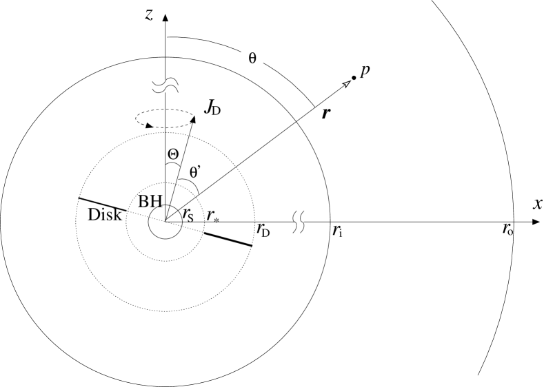
Figure 1.— Basic model configuration. A super massive blackhole (BH) with its Schwarzschild radius $r_{S}$ is located at the center of the cartesian coordinate system ($x$, $y$, $z$) where the $y$-axis is perpendicular to and into the page. The normal vector or the angular momentum ($\boldsymbol{J}_{\mathrm{D}}$) of the accretion disk, spanning from its inner radius $r_{*}$ to its outer radius $r_{D}$, is misaligned with the $z$-axis by a tilt angle $\Theta$ i.e., the accretion disk is tilted by $\Theta$ from the $x$-$y$ plane. The accretion disk hence its angular momentum $\boldsymbol{J}_{\mathrm{D}}$ is assumed to precess around the $z$-axis with the precession period $P$. The 3-D hydrodynamic simulations are performed in the spherical coordinate system ($r$, $\theta$, $\phi$). The simulations are performed in the radial range between the inner boundary $r_{\mathrm{i}}$ and the outer boundary $r_{\mathrm{o}}$. The radiation pressure from the central BH on a point $p$ with its position vector $\boldsymbol{r}$ is in radial direction, and is a function of $r$. Whereas the radiation pressure from the accretion disk is assumed to be a function of $r$ and $\theta^{\prime}$ where the latter is the angle between $\boldsymbol{J}_{\mathrm{D}}$ and $\boldsymbol{r}$ (see Secs. 2.2 and 2.3 for details). The point-source like approximation for the disk radiation pressure at $P$ is valid when $r_{\mathrm{D}}\ll r_{\mathrm{i}}$. Note that the figure is not to scale.

2.1. Hydrodynamics

We employ 3-D hydrodynamical simulations of the outflow from and accretion onto a central part of AGN, using the ZEUS-MP code (c.f., Hayes et al., 2006) which is a massively parallel MPI-implemented version of the ZEUS-3D code (c.f., Hardee & Clarke 1992; Clarke 1996). The ZEUS-MP is a Eulerian hydrodynamics code which uses the method of finite differencing on a staggered mesh with a second-order-accurate, monotonic advection scheme (Hayes et al., 2006). To compute the structure and evolution of a flow irradiated by a strong continuum radiation of AGN, we solve the following set of HD equations:

$$\frac{D\rho}{Dt}+\rho\,\boldsymbol{\nabla}\cdot\boldsymbol{v} = 0,$$ (1)

$$\rho\frac{D\boldsymbol{v}}{Dt}=-\boldsymbol{\nabla}P+\rho\,\boldsymbol{g}+\rho\,\boldsymbol{g}_{\mathrm{rad}},$$ (2)

$$\rho\frac{D}{Dt}\left(\frac{u}{\rho}\right)=-P\,\boldsymbol{\nabla}\cdot\boldsymbol{v}+\rho\,\mathcal{C},$$ (3)

where $\rho$, $u$, $P$ and $\boldsymbol{v}$ are the mass density, energy density, pressure, and the velocity of gas respectively. Also, $\boldsymbol{g}$ is the gravitational force per unit mass. The Lagrangian/co-moving derivative is defined as $D/Dt\equiv\partial/\partial t+\boldsymbol{v}\cdot\boldsymbol{\nabla}$. We have introduced two new components to the ZEUS-MP in order to treat the gas dynamics more appropriate for the gas flow in and around AGN. The first is the acceleration due to radiative force per unit mass ($\boldsymbol{g}_{\mathrm{rad}}$) in equation (2), and the second is the the effect of radiative cooling (and heating) simply as the net cooling rate ($\mathcal{C}$) in equation (3). As this is our first 3-D simulations with this code, we consider a simplest case i.e., $\mathcal{C}=0$ , but $g_{\mathrm{rad}}\neq 0$. We also use $\gamma=1.01$ in the equation of state $P=\left(\gamma-1\right)u$ where $\gamma$ is the adiabatic index. In the following, our implementation of $\boldsymbol{g}_{\mathrm{rad}}$ will be described.

2.1.1 Radiation Force

To evaluate the radiative acceleration due to line absorption/scattering, we follow the method in Proga et al. (2000) who applied the modified Castor, Abbott & Klein (CAK) approximation (Castor et al., 1975). Their model works under the assumption of the Sobolev approximation (e.g., Sobolev 1957; Castor 1970; Lucy 1971); hence, the following conditions are assumed to be valid: (1) presence of large velocity gradient in the gas flow, and (2) the intrinsic line width is negligible compared to the Doppler broadening of a line. Following Proga et al. (2000), the radiative acceleration of a unit mass at a point $\boldsymbol{r}$ can be written as

$$\boldsymbol{g}_{\mathrm{rad}}=\oint_{\Omega}\left[1+\mathcal{M}\right]\left[\frac{\sigma_{e}I\left(\boldsymbol{r},\hat{\boldsymbol{n}}\right)}{c}\right]\hat{\boldsymbol{n}}\,d\Omega$$ (4)

where $I$ is the frequency-integrated continuum intensity in the direction $\hat{\boldsymbol{n}}$, and $\Omega$ is the solid angle subtended by the source of continuum radiation. Also, $\sigma_{e}$ is the electron scattering cross section. The force multiplier $\mathcal{M}$ is a function of optical depth parameter $\tau$ which is similar to the Sobolev optical depth (c.f. Rybicki & Hummer 1978), and can be written as

$$\tau=\frac{\sigma_{e}\,\rho\,v_{\mathrm{th}}}{\left|Q\right|}$$ (5)

where $Q=dv_{l}/dl$ is the directional derivative of the velocity field in direction $\hat{\boldsymbol{n}}$, $dl$ is the line element in the same direction, and $v_{\mathrm{th}}$ is the thermal velocity of the gas. Further equation (4) can be simplified greatly when the continuum radiation source is approximated as a point, i.e., when $r\gg r_{\mathrm{c}}$ where $r_{\mathrm{c}}$ is the radius of the radiation source. In our case, we consider the accretion disk which emits most of the radiation from the innermost part, between $r_{*}$ and $r_{\mathrm{D}}$ in Figure 1; hence, the condition $r\gg r_{\mathrm{c}}$ is satisfied. Using this approximation, the radiative acceleration $\boldsymbol{g}_{\mathrm{rad}}$ will be radial only, and be a function of radial position and polar angle (if the contribution from the disk luminosity is included), i.e. $\boldsymbol{g}_{\mathrm{rad}}=g_{\mathrm{rad}}\left(r,\theta\right)\hat{\boldsymbol{r}}$. This simplification is very useful for our purposes as it reduces the computational time significantly hence it enables us to perform large-scale 3-D simulations. Unlike Proga et al. (2000), we consider the case in which the radiative acceleration is dominated by the continuum process, i.e. $\mathcal{M}=0$ in equation (4) in this paper since we initially intend to investigate the basic characteristics of the impact of the disk precession that do not depend on the details of the radiation force model. The models with $\mathcal{M}\neq 0$ in equation (4) and $\mathcal{C}\neq 0$ will be presented in a forthcoming paper.

2.2. Continuum Radiation Source

As mentioned earlier, we consider two different continuum radiation sources in our models: (1) the accretion disk, and (2) the central spherical corona. Since the geometry of the central engine in AGN is not well understood, we assume that is consist of a spherically shaped corona with its radius $r_{*}$ and the innermost part of the accretion disk (c.f. Fig. 1). The disk is assumed to be flat, Keplerian, geometrically-thin and optically thick. The disk radiation is assumed to be dominated by the radiation from the disk radius between $r_{*}$ and $r_{\mathrm{D}}$ where $r_{*}=3\,r_{\mathrm{S}}$ and $r_{*}<r_{\mathrm{D}}\ll r_{\mathrm{i}}$ (c.f., Fig. 1). Note that the exact size of $r_{\mathrm{D}}$ does not matter as long as it satisfies this condition in order for the point-source approximation mentioned in §. 2.1 to be valid.

In terms of the disk mass-accretion rate ($\dot{M}_{\mathrm{D}}$), the mass of the BH ($M_{\mathrm{BH}}$) and the Schwarzschild radius ($r_{\mathrm{S}}$), the total luminosity ($L$) of the system can be written as

$$L =\eta\dot{M}_{\mathrm{D}}c^{2}$$ (6)

$$=\frac{2\eta GM_{\mathrm{BH}}\dot{M}_{\mathrm{D}}}{r_{\mathrm{S}}}$$ (7)

where $\eta$ is the rest mass conversion efficiency (e.g., Shakura & Sunyaev 1973). Following Proga (2007) and Proga et al. (2007), we simply assume the system essentially radiates only in the UV and the X-ray bands. The total luminosity of the system $L$ is then the sum of the UV luminosity $L_{\mathrm{UV}}$ and the X-ray luminosity $L_{\mathrm{X}}$ i.e., $L=L_{\mathrm{UV}}+L_{\mathrm{X}}$. Further, we assume that the disk only radiates in the UV and the central corona in the X-ray. The ratio of the disk luminosity ($L_{\mathrm{D}}$) to the total luminosity is parametrized as $f_{\mathrm{D}}=L_{\mathrm{D}}/L$, and that of the corona luminosity ($L_{*}$) to the total luminosity as $f_{*}=L_{*}/L$. Consequently, $f_{\mathrm{D}}+f_{*}=1$.

In the point-source approximation limit, the radiation flux from the central X-ray corona region can be written as

$$\mathcal{F}_{*}=\frac{L_{*}}{4\pi r^{2}}$$ (8)

where $r$ is the radial distance from the center (by neglecting the source size). Here we neglect the geometrical obscuration of the corona emission by the accretion disk and vice versa. On the other hand, the disk radiation depends on the polar angle $\theta$ because of the source geometry. Again following Proga (2007) and Proga et al. (2007) (see also Proga et al. 1998), the disk intensity $I_{\mathrm{D}}$ is assumed to be radial and $I_{\mathrm{D}}\propto\left|\cos\theta^{\prime}\right|$. This follows that the disk radiation flux at the distance $r$ from the center can be written as

$$\mathcal{F}_{\mathrm{D}}=2\,\left|\cos\theta^{\prime}\right|\,\frac{L_{\mathrm{D}}}{4\pi r^{2}}$$ (9)

where $\theta^{\prime}$ is the angle between the disk normal and the position vector $\boldsymbol{r}$ (c.f., Fig. 1). The leading term $2$ in this expression comes from the normalization of the polar angle dependency. Finally by using eqs. (4), (8) and (9), the radiative acceleration term in equation (3) can be written as

$$\boldsymbol{g}_{\mathrm{rad}}=\frac{\sigma_{e}L}{4\pi r^{2}c}\left\{f_{*}+2\,\left|\cos\theta^{\prime}\right|\,f_{\mathrm{D}}\right\}\,\boldsymbol{\hat{r}}\,.$$ (10)

2.3. Precessing Disk

As we noted before, here we do not model the precession of the accretion disk itself, but rather manually force the precession. We do not specify the cause of the precession either. We simply assume that the disk precession exists, and investigate its consequence to the AGN environment. The UV emitting portion of the disk spans from $r_{*}$ to $r_{\mathrm{D}}$ (c.f., Fig. 1). We assume that $r_{\mathrm{D}}\ll r_{\mathrm{i}}$ where the $r_{\mathrm{i}}$ is the inner radius of the computational domain of the hydrodynamic simulations. This means that the disk itself is not in the computational domain. The effect of the precessing disk is included as precessing radiation field in the hydrodynamics of the gas (through eq. [2]).

We assume that the disk is tilted from the $x$-$y$ plane (in the cartesian coordinate system) by $\Theta$ as in Figure 1. Equivalently, the disk angular momentum $\boldsymbol{J}_{\mathrm{D}}$ (assuming a flat uniform Keplerian disk) deviates from the $z$-axis by $\Theta$. Further, we assume that $\boldsymbol{J}_{\mathrm{D}}$ precesses around the $z$-axis with precession period $P$. With these assumptions, the components of the $\boldsymbol{J}_{\mathrm{D}}$ in the cartesian coordinate system can be written as

$$J_{\mathrm{D}x} =J_{D}\sin\Theta\,\cos\left(\frac{2\pi t}{P}\right),$$ (11)

$$J_{\mathrm{D}y} =J_{D}\sin\Theta\,\sin\left(\frac{2\pi t}{P}\right),$$ (12)

$$J_{\mathrm{D}z} =J_{D}\cos\Theta$$ (13)

where $t$ is the time measured from the beginning of hydrodynamic simulations. Here we set $\boldsymbol{J}_{\mathrm{D}}$ to be on the $x-z$ plane (as shown in Fig. 1) at $t=0$. By setting $\Theta=0$, the model reduced to an asymmetric case as in Proga (2007). To compute the radiative acceleration as expressed in equation (10), one requires the angle between $\boldsymbol{J}_{\mathrm{D}}$ and the position vector $\boldsymbol{r}$ at which the set of the HD equations (eqs. [1], [2] and [3]) are solve. This can be obtained simply by finding the inner product of $\boldsymbol{J}_{\mathrm{D}}$ and $\boldsymbol{r}$.

2.4. Model Setup

In all models presented here, the following ranges of the coordinates are adopted: $r_{\mathrm{i}}\leq r\leq r_{\mathrm{o}}$, $0\leq\theta\leq\pi$ and $0\leq\phi<2\pi$ where $r_{\mathrm{i}}=500\,r_{*}$ and $r_{\mathrm{o}}=2.5\times 10^{5}\,r_{*}$. The radius of the central and spherical X-ray corona region $r_{*}$ coincides with the inner radius of the the accretion disk (Fig. 1). In our simulations, the polar and azimuthal angle ranges are divided into 128 and 64 zones, and are equally spaced. In the $r$ direction, the gird is divided into 128 zones in which the zone size ratio is fixed at $\Delta r_{k+1}/\Delta r_{k}=1.04$.

For the initial conditions, the density and the temperature of gas are set uniformly i.e., $\rho=\rho_{o}$ and $T=T_{o}$ everywhere in the computational domain where $\rho_{o}=1.0\times 10^{-21}\,\mathrm{g\,cm^{-3}}$ and $T_{o}=2\times 10^{7}\,\mathrm{K}$ through out this paper. The initial velocity of the gas is simply set to zero everywhere.

At the inner and outer boundaries, we apply the outflow (free-to-outflow) boundary conditions, in which the field values are extrapolated beyond the boundaries using the values of the ghost zones residing outside of normal computational zones (see Stone & Norman 1992 for more details). At the outer boundary, all HD quantities (except the radial velocity) are fixed constant, to their initial values (e.g., $T=T_{o}$ and $\rho=\rho_{o}$), during the the evolution of each model. The radial velocity components are allowed to float. Proga (2007) applied these conditions to represent a steady flow condition at the outer boundary. They found that this technique leads to a solution that relaxes to a steady state in both spherical and non-spherical accretion with an outflow (see also Proga & Begelman 2003). This imitates the condition in which a continuous supply of gas is available at the outer boundary.

3. Results

3.1. Reference Values

Table 1Model Summary

	$\Theta$	$P$	$\dot{M}_{\mathrm{in}}\left(r_{\mathrm{o}}\right)$	$\dot{M}_{\mathrm{net}}\left(r_{\mathrm{i}}\right)$	$\dot{M}_{\mathrm{out}}\left(r_{\mathrm{o}}\right)$	$v_{r}^{\mathrm{max}}\left(r_{\mathrm{o}}\right)$	$P_{k}\left(r_{\mathrm{o}}\right)$	$P_{\mathrm{th}}\left(r_{o}\right)$	$j_{\rho}$
Model	$\left(\,{}^{\circ}\right)$	$\left(\mathrm{yr}\right)$	$\left(10^{25}\mathrm{\,g\,s^{-1}}\right)$	$\left(10^{25}\,\mathrm{g\,s^{-1}}\right)$	$\left(10^{25}\,\mathrm{g\,s^{-1}}\right)$	$\left(\mathrm{km\,s^{-1}}\right)$	$\left(10^{40}\,\mathrm{erg\,s^{-1}}\right)$	$\left(10^{40}\,\mathrm{erg\,s^{-1}}\right)$	$\left(j_{0}\right)$
I	$0$	$\infty$	$-2.2$	$-0.6$	$1.6$	$1500$	$3.0$	$260$	$0$
II	$5$	$1.6\times 10^{4}$	$-2.3$	$-0.6$	$1.7$	$640$	$1.4$	$290$	$0.2$
III	$15$	$1.6\times 10^{4}$	$-2.2$	$-0.4$	$1.8$	$620$	$1.1$	$310$	$0.2$
IV	$5$	$1.6\times 10^{5}$	$-2.2$	$-0.6$	$1.6$	$1900$	$3.0$	$260$	$0.05$

We consider four different cases which have different combinations of the disk tilt angle ($\Theta$) and the disk precession period ($P$), as summarized in Table 1. The following parameters are common to all the models presented here, and are exactly the same as in Proga (2007). We assume that the central BH is non-rotating and has mass $M_{\mathrm{BH}}=10^{8}\,M_{\odot}$. The size of the disk inner radius is assumed to be $r_{*}=3r_{s}=8.8\times 10^{13}\,\mathrm{cm}$ (c.f. Sec. 2.4). The mass accretion rate ($\dot{M}_{a}$) onto the central SMBH and the rest mass conversion efficiency ($\eta$) are assumed to be $1\times 10^{26}\,\mathrm{g\,s^{-1}}$ and $0.0833$, respectively. With these parameters, the corresponding accretion luminosity of the system is $L=7.5\times 10^{45}\,\mathrm{erg\,s^{-1}=2\times 10^{12}\,L_{\sun}}$. Equivalently, the system has the Eddington number $\Gamma=0.6$ where $\Gamma\equiv L/L_{\mathrm{Edd}}$ and $L_{\mathrm{Edd}}$ is the Eddington luminosity of the Schwarzschild BH i.e., $4\pi cGM_{\mathrm{BH}}/\sigma_{e}$. The fractions of the luminosity in the UV ($f_{\mathrm{UV}}$) and that in the X-ray ($f_{\mathrm{X}}$) are fixed at $0.95$ and $0.05$ respectively, as in Proga (2007) (see their Run C).

Important reference physical quantities relevant to our systems are as follows. The Compton radius, $R_{C}\equiv GM_{\mathrm{BH}}\mu\,m_{p}/kT_{C}$, is $8\times 10^{18}\,\mathrm{cm}$ or equivalently $9\times 10^{4}\,r_{*}$ where $T_{C}$, $\mu$ and $m_{p}$ are the Compton temperature, the mean molecular weight of gas and the proton mass, respectively. Here we assume that the gas temperature at infinity is $T_{\infty}=T_{C}=2\times 10^{7}\,\mathrm{K}$; hence, the corresponding speed of sound at infinity is $c_{\infty}=(\gamma kT_{C}/\mu m_{p})^{1/2}=4\times 10^{7}\,\mathrm{cm\,s^{-1}}$ where $\gamma$ is the adiabatic index. In this paper, $\gamma=1.01$ (almost isothermal) is adopted to imitate a gas in Compton equilibrium with the radiation field. The corresponding Bondi radius (Bondi, 1952) is $R_{B}=GM_{\mathrm{BH}}/c_{\infty}^{2}=4.8\times 10^{18}\,\mathrm{cm}$ while its relation to the Compton radius is $R_{B}=\gamma^{-1}R_{C}$. The Bondi accretion rate (for the isothermal flow) is $\dot{M}_{B}=3.3\times 10^{25}\,\mathrm{g\,s^{-1}}=0.52\,\mathrm{M_{\sun}\,yr^{-1}}$. The corresponding free-fall time ($t_{\mathrm{ff}}$) of gas from the Bondi radius to the inner boundary is $2.1\times 10^{11}\,\mathrm{sec}=7.0\times 10^{3}\,\mathrm{yr}$ which is about $2.3$ times smaller than the precession period used for Models II and III, and about $23$ times smaller than that of Model IV (c.f. Tab. 1).

3.2. Comparison of axisymmetric models in 2-D and 3-D

Before we proceed to the main precession disk models, we briefly compare our axisymmetric model (Model I) with the axisymmetric models presented earlier by Proga (2007) who used very similar model parameters as in our Model I. The main differences here are in the treatment of the radiation force and that in the radiative heating/cooling. As mentioned earlier, we set the force multiplier $\mathcal{M}=0$ (in eq. [4]) and the net cooling rate $\mathcal{C}=0$ (in eq. [3]) while Proga (2007) used non-zero values of those two terms. In our Model I, the adiabatic index is set to $\gamma=1.01$ (essentially isothermal), but their models use $\gamma=5/3$. However, Proga (2007) found that their Run A is nearly isothermal despite $\gamma=5/3$ was used (see their Fig. 1). Another important difference is the numerical codes used. Proga (2007) used the ZEUS-2D code (Stone & Norman, 1992).

Overall geometry of the flow in Model I (Figs. 2 and 3) is similar to those in Proga (2007). The matter accretes onto the central BH near the equatorial plane, and strong outflows occur in polar direction. The collimation of our model is relatively weak compared to their Run C which uses exactly the same disk and corona luminosities as in our Model I. The wider bipolar outflow pattern seen here resembles that of their Run A which has the highest X-ray heating. The difference and the resemblance seen here are caused by the following two key factors: (1) nearly isothermal equation of state and (2) no radiative cooling ($\mathcal{C}=0$) in our model . These condition keep the temperature of gas warm everywhere in the computational domain, and the temperature is essentially that set at the outer boundary ($T_{\infty}=T_{C}=2\times 10^{7}\,\mathrm{K}$). This will result in a very similar situation as in Run A of Proga (2007) in which the gas temperature is also relatively high because of the high X-ray heating and cooling. The high temperature hence the ionization state of the gas makes the line force in their model very inefficient, resulting in the situation in which the gas is almost entirely driven by the continuum process (electron scattering) and thermal effects just as in our Model I.

Although not shown here, we have also checked the internal consistency of the ZEUS-MP (3-D) code by running the axisymmetric models (Model I) in both 2-D and 3-D modes. We find that the results from the both runs agree with each other in all aspects e.g., inflow and outflow geometry, density distribution, velocity, mass accretion and outflow rates.

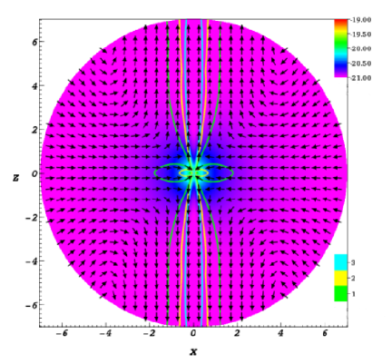
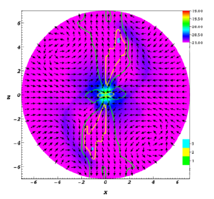
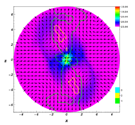
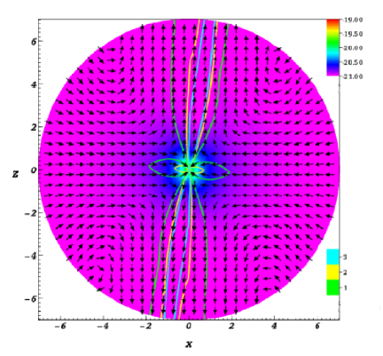
Figure 2.— Comparison of the density and velocity fields on the $x$-$z$ plane from Models I (upper-left) II (upper-right), III (lower-left) and IV (lower-right). The density maps shown in the background are given in logarithmic scale (base 10) and in cgs units. The contours of the Mach number are overlaid along with the arrows which indicate the directions of the velocity on the x-$z$ plane. The units of both $x$ and $z$ axes are in pc. The time slices of each models are chosen such that the density and velocity fields are representative of each model.

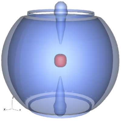
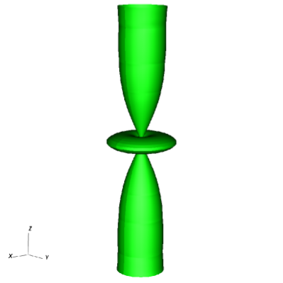
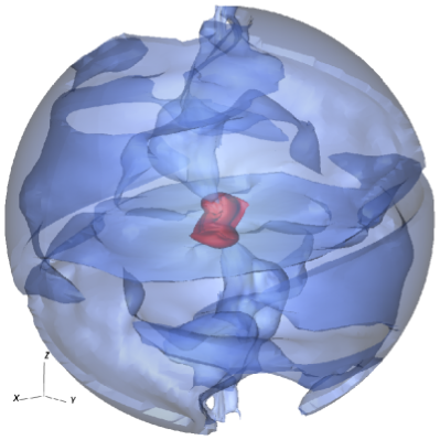
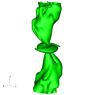
Figure 3.— Two-level iso-density (left panels) and the corresponding sonic (right panels) surfaces in 3-D for Models I (upper panels) and II (lower panels). The density levels used here are $\log\,\rho=-20.5$ (blue) and $-21$ (red) where $\rho$ is in $\mathrm{g\,cm^{-3}}$. The time slices of the simulation data used here are as in Fig. 2. The sizes of the plotting boxes are $14.2$ pc in all directions ($x$, $y$ and $z$).

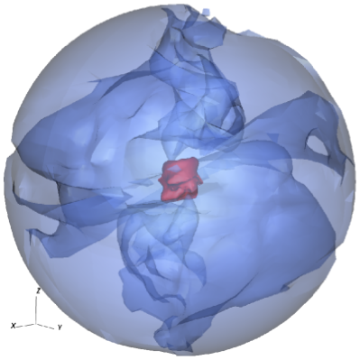
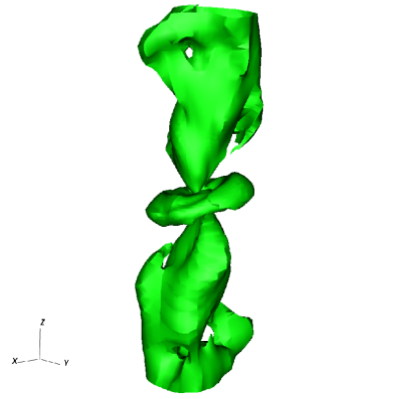
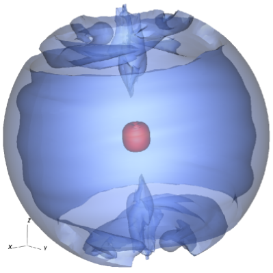
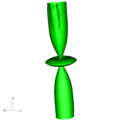
Figure 4.— As in Fig. 3, but for Models III and IV.

3.3. Dependency on the disk tilt angle $\Theta$

We now examine the model dependency on disk tilt angle ($\Theta$) while keeping all other parameters fixed. The results from Models I, II and III (c.f.,  Tab 1), which use $\Theta=0^{\circ}$, $5^{\circ}$ and $15^{\circ}$ respectively, are compared for this purpose. Note that the observations suggest that a large fraction of AGN have rather small i.e., $\Theta<\sim 15^{o}$ (e.g., Lu & Zhou 2005).

Figure 2 shows the slices of the density and velocity fields (on the $y=0$ plane) from snapshots of our four simulations. The snapshots are chosen at the time when the models reached a (semi-)steady state for Models I and II. As we will see later, the flow never reaches steady state in Model III; therefore, we chose the snapshot of the model at the time when the flow pattern is a typical of a whole simulation time sequence. While accretion occurs mainly on the equatorial plane ($z=0$) for Model I, it occurs in a inclined plane with a pitch angle (a angle between the equatorial plane and the accretion plane) similar to the disk inclination angle, for Models II and III. In the precessing disk models (II and III), the deviation from the axisymmetric is clearly seen in both density distribution of gas and the shapes of the Mach number contours. Corresponding 3-D density and Mach number contour surfaces of these models are also shown in Figs. 3 and 4. The morphology of the density distribution seen in Figure 2 resemble that of the Z-shaped (for Model II) and the S-shaped (for Model III) radio jets (e.g. Condon & Mitchell 1984; Hunstead et al. 1984; Tremblay et al. 2006) although in different scales. Obviously, the difference between the Z- and S- shapes are simply due to the difference in the viewing angles. Unlike the MHD precessing jet models, the bending structures of the density distributions seen here are shaped by the geometry of the sonic surfaces. When accreting material from the outer boundary encounters the relatively low density but high-speed outflowing gas launched by the radiation force from the inner part, the gas becomes compressed, and forms higher density regions. The flows in the bending density structure itself are rather complex (especially in Model III), but the direction of the flow becomes outward (in radial direction) as they approach the sonic surface (excluding the one shaped like a disk formed by the accreting gas in the inner region). Relatively large curvatures of the flows seen in both density and the Mach number contours of Models II and III can be also understood from the fact the precession period used in these models ($P=16000\,\mathrm{yr}$) is comparable to the gas free fall time ($t_{\mathrm{ff}}=7000\,\mathrm{yr}$, c.f., § 3.1). The curvatures or the “twists” of the weakly collimated bipolar flows can be clearly seen in the 3-D representation of these models in Figs. 3 and 4.

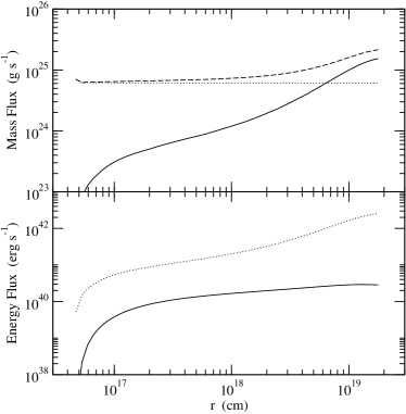
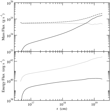
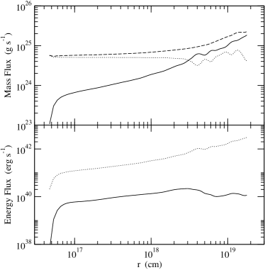
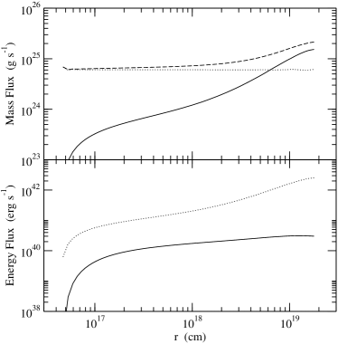
Figure 5.— Comparison of mass flux and energy flux as a function of radius for Models I (upper-left), II (upper-right), III (lower-left) and IV (lower-right). The plot for each model is subdivided into two panels: top (mass flux) and bottom (energy flux). In the mass flux plots, the inflow (dash: $\dot{M}_{\mathrm{in}}$), outflow (solid: $\dot{M}_{\mathrm{o}}$) and net (dot: $\dot{M}_{\mathrm{net}}$) mass fluxes, as defined in equation (15), are separately plotted as a function of radial distance from the center. The absolute values of $\dot{M}_{\mathrm{in}}$ and $\dot{M}_{\mathrm{net}}$ are plotted here since they are negative at all radii. In the energy flux plots, the kinetic energy (solid) and the thermal energy (dot), defined in eqs. (16) and (17), are shown. Note that the times slices of the model simulations used here to computed the fluxes are same as those in Figure 2.

We compute the mass fluxes as a function of radius for a quantitative comparison of the characteristics of the flows in the models. Following Proga (2007), the net mass flux ($\dot{M}_{\mathrm{net}}$), the inflow mass flux ($\dot{M}_{\mathrm{in}}$) and the outflow mass flux ($\dot{M}_{\mathrm{out}}$) can be computed from

$$\dot{M}\left(r\right) =\oint_{s}\rho\,\boldsymbol{v\,\cdot}d\boldsymbol{a}$$ (14)

$$=r^{2}\oint_{4\pi}\rho v_{r}\,d\Omega$$ (15)

where $v_{r}$ is the radial component of velocity $\boldsymbol{v}$. In the equation above, $\dot{M}=\dot{M}_{\mathrm{net}}$ if all $v_{r}$ are included. Similarly, $\dot{M}=\dot{M}_{\mathrm{in}}$ for $v_{r}<0$ and $\dot{M}=\dot{M}_{\mathrm{out}}$ for $v_{r}>0$. Also, $d\boldsymbol{a}=\boldsymbol{\hat{r}}\,r^{2}\sin\theta\,d\theta\,d\phi$ and $d\Omega=\sin\theta\,d\theta\,d\phi$. Similarly we further define the outflow power in the form of kinetic energy ($P_{k}$) and that in the thermal energy ($P_{\mathrm{th}}$) as functions of radius i.e.,

$$P_{k}\left(r\right) =r^{2}\oint_{4\pi}\rho v_{r}^{3}\,d\Omega$$ (16)

and

$$P_{\mathrm{th}}\left(r\right) =r^{2}\oint_{4\pi}uv_{r}\,d\Omega\,.$$ (17)

where $v_{r}>0$.

The resulting mass fluxes and the outflow powers of the models are summarized in Figure 5. In all cases, the mass inflow flux exceeds the mass outflow rate at all radii. For Models I and II, the net mass fluxes ($\dot{M}_{\mathrm{net}}$) are almost constant at all radii, indicating that the flows in these models are steady. Despite the presence of the disk precession in Model II, the flow becomes steady. The density distribution and the velocity field become almost constant in the coordinate system co-rotating with the disk precession period. On the other hand, $\dot{M}_{\mathrm{net}}$ for Model III does not remain constant as $r$ becomes larger ($r>10^{18}\,\mathrm{cm}$) because of the unsteady nature of the flow (c.f., Figs. 2 and 4). As the disk tilt angle $\Theta$ increases, the direction of the outflows, which are normally in polar directions ($\pm z$ directions) with an absence of the disk tilt, moves toward the equatorial plane (the $x$-$z$ plane) where the flow is predominantly inward. This opposite flows makes it harder for the outflowing gas to reach the outer boundary. Further, since the disk is precessing, the direction of the outflow is constantly changing. This results in continuous collisions between the inflowing and outflowing gas especially for a larger $\Theta$ model. The net mass fluxes at the inner boundary $\dot{M}_{\mathrm{net}}\left(r_{\mathrm{i}}\right)$ are $-0.6$, $-0.6$ and $-0.4\times 10^{25}\,\mathrm{g\,s^{-1}}$ (or equivalently $-0.10$, $-0.1$0 and $-0.06$ $\mathrm{M_{\sun}\,yr^{-1}}$) for Models I, II and III respectively (Tab. 1), indicating the net mass flux inward (negative signs indicate inflow) decreases slightly, but not significantly as the disk tilt angle $\Theta$ increases.

The ratios of the total mass outflow flux to the total mass inflow at the outer boundary ($\mu=\left|\dot{M}_{\mathrm{out}}/\dot{M}_{\mathrm{in}}\right|$) are $0.7$3, $0.74$, $0.82$ for Models I, II, and III (see also Tab. 1). These values indicates that the high efficiency of the outflow by the radiation pressure even for a modest Eddington number used here i.e., $\Gamma=0.6$. This conversion efficiency $\mu$ (from the outflow to inflow) is about the same for Models I and II, but it slightly ($\sim 12$%) increases for Model III which has the highest disk tilt angle. Overall characteristics of the mass-flux curves as a function radius for Models I and II are also very similar to each other. The curves for Model III are also similar to those of Models I and II; however, they differ in the outer radii ($r<\sim 10^{18}\mathrm{cm}$), mainly because of the unsteady nature of the flow in this model.

The maximum speed of the outflow in the radial direction $v_{r}^{max}\left(r_{\mathrm{\mathrm{o}}}\right)$ decreases as $\Theta$ increases (Tab. 1). The reduction in the speed is very significant ($\Delta v_{r}=-860\,\mathrm{km~{}s^{-1}}$) as $\Theta$ increase from $0^{\circ}$ to $5^{\circ}$ while the change is relatively small ($\Delta v_{r}=-20\,\mathrm{km~{}s^{-1}}$) as $\Theta$ changes from $5^{\circ}$ to $15^{\circ}$.

Figure 5 also shows the outflow powers ($P_{k}$ and $P_{\mathrm{th}}$) of the models as a function of radius, as defined in eqs. (16) and (17). As for the mass flux curves in the same figure, the dependency of the energy flux curves on radius for Models I, II and III are very similar to each others. A small but noticeable deviations of the curves for Model III from those for Models I and II are seen at the large radii ($r>3\times 10^{18}\,\mathrm{cm}$). The figure shows that in all three models, the outflow power is dominated by thermal process ($P_{\mathrm{th}}\approx 10-100\,P_{k}$ at all radii). This can be explained by the high temperatures of the gas ($T\approx T_{C}=2.0\times 10^{7}\,\mathrm{K}$ ) in the computational domains caused by the (almost) isothermal equation of state and the temperature ($2.0\times 10^{7}\,\mathrm{K}$) fixed at the outer boundary. The kinetic powers or the radiation forces are not as significant as the pressure gradient force in these models; however, their importance cannot be ignored since they “shape” the geometry of the outflow as they strongly depend on the polar angle position of a point in the computational field. We also note that as $\Theta$ increases, the kinetic power at the outer boundary $P_{k}\left(r_{\mathrm{o}}\right)$ decreases significantly e.g. $P_{k}\left(r_{\mathrm{o}}\right)$ of Model III is three times smaller than that of the axisymmetric model, Model I (see Table 1).

Next we examine the degree of non-axisymmetry in Model I, II and III, and seek for any obvious dependency on $\Theta$. For this purpose, we compute the center of mass (CM) of the gas on the planes perpendicular to the $z$-axis (as a function of $z$) i.e., $x_{c}\left(z\right)$ and $y_{c}\left(z\right)$ which are defined as

$$x_{c}\left(z\right)=\frac{\int_{-r_{\mathrm{o}}}^{r_{\mathrm{o}}}\int_{-a}^{a}\int_{-\infty}^{\infty}x\,\delta\left(z-z^{\prime}\right)\rho\left(x,y,z^{\prime}\right)dz^{\prime}\,dx\,dy}{m\left(z\right)}$$ (18)

and

$$y_{c}\left(z\right)=\frac{\int_{-r_{\mathrm{o}}}^{r_{\mathrm{o}}}\int_{-a}^{a}\int_{-\infty}^{\infty}y\,\delta\left(z-z^{\prime}\right)\rho\left(x,y,z^{\prime}\right)dz^{\prime}\,dx\,dy}{m\left(z\right)}$$ (19)

where

$$m\left(z\right)=\int_{-r_{\mathrm{o}}}^{r_{\mathrm{o}}}\int_{-a}^{a}\int_{-\infty}^{\infty}\delta\left(z-z^{\prime}\right)\rho\left(x,y,z^{\prime}\right)dz^{\prime}\,dx\,dy\,\,,$$ (20)

and $a\left(y,z\right)=$ $\left(r_{\mathrm{o}}^{2}-z^{2}-y^{2}\right)^{1/2}$. The results are shown in Figure 6. As expected, the CM position remains constant and on the $z$-axis ($x_{c}\left(z\right)=0$ and $y_{c}\left(z\right)=0$) for Model I, as this is an axisymmetric model. For both Models II and III, the maximum amount of deviations for each component of the CM ($\left|x_{c}\right|$and $\left|y_{c}\right|$) is about $0.3$ pc which is relatively small compared to the outer boundary radius ($r_{\mathrm{o}}=7.1\,\mathrm{pc}$). The $x_{c}$ and $y_{c}$ curves are anti-symmetric about the $z=0$ position since our model accretion disk hence the radiation force is symmetric about the origin of the coordinate system. The plot also shows that the positions of the maxima and minima in the $x_{c}$ and $y_{c}$ curves do not coincide, but they are rather shifted in both $+z$ and $-z$ directions. This clearly demonstrates a helical or twisting nature of the flows, as one can also simply see it in the 3-D density and Mach number contour plots in Figs. 3 and 4.

To summarize, as the tilt angle of the disk precession $\Theta$ increases, reductions of the maximum outflow velocity ($v_{r}$) and the kinetic outflow power ($P_{k}$) at the outer boundary $r_{\mathrm{o}}$ occur, as a consequence of the stronger interactions between the outflowing and inflowing gas of as $\Theta$ increases. The net mass inflow flux ($\dot{M}_{\mathrm{net}}$) at the inner boundary does not strongly depend on $\Theta$. The thermal outflow energy power dominates the kinetic outflow power in our models here because of the high temperature of set at the outer boundary and because the gas is (almost) isothermal. The flows of Models II and III show helical structures; however, the radius of the helices (base on the CM positions along the z-axis) does not change greatly as $\Theta$ increases from $5^{\circ}$ to $15^{\circ}$.

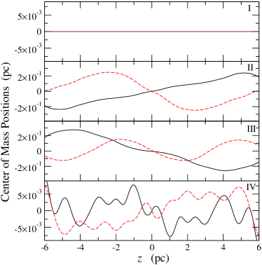
Figure 6.— Positions of the center of mass of the gas on the planes perpendicular to the $z$-axis for Models I, II, III and IV from the top bottom. The locations of the center of mass, $x_{c}$ (sold) and $y_{c}$ (dash) as defined in eqs. (18) and (19), are computed as a function of $z$. All models except Model I show a clear sign of deviations from axisymmetry; however the displacement of the center of mass remains fairly small ($\left|x_{c}\right|<\sim 0.3\,\mathrm{pc}$ and $\left|y_{c}\right|<\sim 0.3\,\mathrm{pc}$), at all $z$ locations, compared to the size of outermost radius $r_{\mathrm{o}}$ ($7.1$ pc) of the computational domain. The patterns in $x_{c}$ and $y_{c}$ curves for Models II and III indicate that the flow density structures are helical.

3.4. Dependency on the disk precession period $P$

We now examine the dependency of the model on the disk precession period ($P$). We vary the value of $P$ while fixing the disk tilt angle to $\Theta=5^{\circ}$. For this purposed, we compare Models I, II and IV as summarized in Table. 1. The precession periods $P$ are $\infty$, $1.6\times 10^{4}$ and $1.6\times 10^{5}$ yr respectively for Models I, II and IV. In the units of the free-fall time ($t_{\mathrm{ff}}=7.0\times 10^{3}$ yr ) from the Bondi radius (§ 3.1), they are $\infty$, $2.3$ and $23$ respectively. Note that the observations suggest that typical values of jet precession period are $P=10^{4}$–$10^{6}$ yr (c.f., Tab.1 in Lu & Zhou 2005).

Figure 2 shows that similarities between Model IV and Model I in their morphology of the density distribution and Mach number surfaces. At a given time, the flow in Model IV is almost axisymmetric, and the symmetry axis is tilted also by $\Theta=5^{\circ}$ from the $z$-axis. This is caused by the relatively long precession period for Model IV compared to the dynamical time scale or the gas free-fall time scale $t_{\mathrm{ff}}$. The curvature or helical motion of the gas is not significant, and it does not greatly affect the overall morphology of the flow, except for the outermost part of the flow where the flow is slightly turbulent due to the shear of the slowly precessing flow and the outer boundary. This can be clearly seen in the 3-D plots Figure 4. As the precession period $P$ becomes shorter and comparable to $t_{\mathrm{ff}}$ (as in Model II), the flow shows more curvature and the helical structures.

The mass flux curves (c.f., eq. [15]) for Models IV in Figure 5 also show that nature of the flows between Models I and IV are very similar to each other. Overall characteristics of the curves are also similar to that of Model II. In fact, the net mass flux $\dot{M}_{\mathrm{net}},$ the inflow mass flux $\dot{M}_{\mathrm{in}}$ and the outflow mass flux $\dot{M}_{\mathrm{out}}$ at the outer boundary of Model IV are identical to those of Model I (see Table 1). Also note that Models I, II and IV all have same $\dot{M}_{\mathrm{in}}$ value at the inner boundary, i.e., the mass inflow rate across the inner boundary in insensitive to the change in the precession period for $\Theta=5^{\circ}$.

The similarity between and Models I and IV can be also seen in the outflow powers, $P_{k}$ and $P_{\mathrm{th}}$. Figure 5 shows $P_{k}$ and $P_{\mathrm{th}}$ as a function of radius for Model IV are almost identical to those of Model I. The $P_{k}$ and $P_{\mathrm{th}}$ values at outer boundary are indeed identical (Table 1). A slight increase in the maximum outflow velocity at the outer boundary $v_{r}^{\mathrm{max}}(r_{\mathrm{o}})$ is observed for Model IV, compared to Model I. The kinetic outflow power $P_{k}$ and the maximum outflow velocity at the outer boundary $v_{r}^{\mathrm{max}}(r_{\mathrm{o}})$ decreases as the precession period become comparable to $t_{\mathrm{ff}}$.

The CM positions $x_{c}$ and $y_{c}$ as a function of $z$ (see § 3.3) for Model IV is shown in Figure 6. Compared to Model II, the maximum displacement of the CM is about 40 times smaller in Model IV i.e. $\left|x_{c}\right|<\sim 0.075\,\mathrm{pc}$ and $\left|y_{c}\right|<\sim 0.075\,\mathrm{pc}$. The $x_{c}$ curve for Model IV shows a rather complex pattern compared to that in Model II. This and the visual inspection of the density and the Mach number contour surfaces in Figure 4, indicates that the bipolar outflow flows are slightly twisted, but does not have clear helical structure.

3.5. Time Evolution of Mass Accretion/Outflow Rates and Angular Momentum

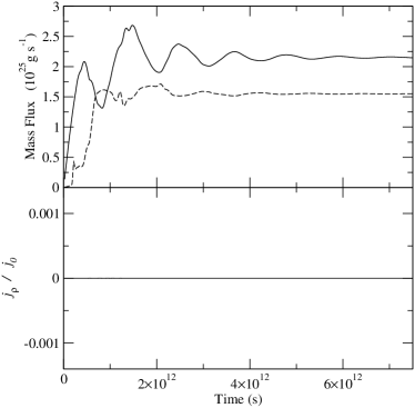
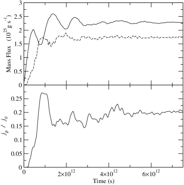
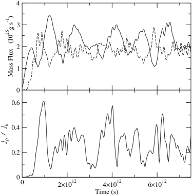
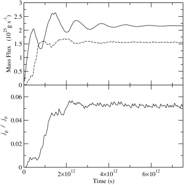
Figure 7.— The mass flow rates across the outer boundary and the density-weighted mean specific angular momentum $j_{\rho}$ (c.f. eqs. [15] and [21]) plotted as a function of time for Models I (upper-left), II (upper-right), III (lower-left), and IV (lower-right). For each model, the plot is subdivided into two panels: mass-inflow/outflow rates (top panels) and $j_{\rho}$ (bottom panels). In the top panels, the mass-inflow rate at the outer boundary (solid), and the mass-outflow rate at the outer boundary (dash) are shown separately. The values of $j_{\rho}$ are in the units of $j_{0}$ which is defined as the specific angular momentum of the gas in Keplerian orbit at the inner boundary ($r=r_{\mathrm{in}}$). Note that the precession period used here are $\infty$, $5.0\times 10^{11}\,\mathrm{s}$, $5.0\times 10^{11}\,\mathrm{s}$ and $5.0\times 10^{12}\,\mathrm{s}$ for Models I, II, III and IV respectively.

Next, we examine the variability or steadiness of the flows in each model by monitoring the mass fluxes at the outer boundary as in equation (15) and the angular momentum of the system as a function of time. For the latter, we compute the density-weighted mean specific angular momentum $\boldsymbol{j}_{\rho}$ of the systems defined as:

$$\boldsymbol{j}_{\rho}=\frac{\int_{V}\rho\,\left(\boldsymbol{r}\times\boldsymbol{v}\right)\,dV}{\int_{V}\rho\,dV}$$ (21)

where the denominator is simply the total mass of the gas in the computational domain. Note that the radiation force (eq. [10]) and the gravitational force are in radial direction only. Consequently, they do not exert torque onto the system; hence, they do not contribute to the change in the angular momentum of the system directly. The system can gain the angular momentum in the following way. In our models, the strength of the disk radiation field depends on the angle measured from the disk normal (c.f., eq. [9]). This causes gas pressure gradients in azimuthal direction, and contributes to the angular momentum of gas locally, forming vorticity. The precession of radiation field hence the precessing outflow will cause the gas with preferred sign of vorticity to escape from the outer boundary, resulting a change in the net angular momentum of the gas in the computational domain.

Figure 7 shows $\dot{M}_{\mathrm{in}}\left(r_{o}\right)$, $\dot{M}_{\mathrm{out}}\left(r_{o}\right)$ and $j_{\rho}$ for Models I, II, III and IV as a function of time. For Models I, II and IV, both the mass fluxes and $j_{\rho}$ reach to asymptotic values by $t\approx 7\times 10^{12}\,\mathrm{s}$. Small oscillations of $j_{\rho}$ around the asymptotic values are seen for Models II and IV. On the other hand, the mass fluxes of Model III has much larger amplitudes of the oscillations around an asymptotic value. By visual inspections, their oscillations do not seem have a clear periodicity associated with them. We performed the Lomb-Scargle periodgram analysis (e.g. Horne & Baliunas 1986; Press et al. 1992) on the $\dot{M}_{\mathrm{in}}\left(r_{o}\right)$, $\dot{M}_{\mathrm{out}}\left(r_{o}\right)$ and $j_{\rho}$ curves for Model III. Only $\dot{M}_{\mathrm{out}}\left(r_{o}\right)$ shows a relatively strong signal at $P_{\mathrm{LS}}=1.36\times 10^{12}\,\mathrm{s}$ which is about $2.7$ times longer than the precession period of Model III. On the other hand $\dot{M}_{\mathrm{in}}\left(r_{o}\right)$ and $j_{\rho}$ curves do not have any obvious period associated with them, but they are rather stochastic.

As mentioned in § 3.3, as the disk tilt angle $\Theta$ increases the direction of the outflows, which normally exists in polar directions with an absence of the disk tilt, moves toward the equatorial plane (the x-$z$ plane) where the flow is predominantly inward. In addition, the precession of the disk causes the direction of the outflow to change constantly; hence, causing constant creation of the shock between the inflowing and the outflowing gas. This leads into a very unstable flow of the gas at all time for a model with a larger $\Theta$ e.g., Model III with $\Theta=15^{\circ}$. The flow, of course, can be stabilized if the precession period is increased to a value much larger than the free-fall time $t_{\mathrm{ff}}$.

The amount of the (density-weighted) mean specific angular momentum deposited to the gas by the precessing disk (measured by $j_{\rho}$) is largest in Models II and III (see Table 1), and that in Model IV is about $4$ times less than those of Models II and III. For all models, a time-averaged value (by using the last $2\times 10^{12}\,\mathrm{s}$ of the simulation) of $j_{\rho}$ is used in Table 1. It seems that the faster the disk precesses, the lager the amount of angular momentum transferred to the environment; however, this trend does not continues, as we increase the disk precession speed even faster. Although not shown here, a model with exactly the same set of parameters as in Model II, but with $P=1600\,\mathrm{yr}$ (10 times faster rotation), showed that the the value of $j_{\rho}$ decrease to $\sim 0.01$, which is even smaller than Model IV (with $P=160000\,\mathrm{yr}$). This indicates that the amount of angular momentum deposited to the gas depends on how close the precession period to the dynamical time scale of the flow.

In principle, it is possible to model the change in the angular momentum of the accretion disk itself through the transfer of angular momentum from the environment, we ignored this effect for simplicity (and this is also our model limitation). To model the interaction of the disk angular momentum and the angular momentum of the surrounding gas properly, we need to model the dynamics of the gas in the accretion disk itself as well as the dynamic of the gas which is much larger scale as in our models here. This is computationally challenging with our current code since we have to resolve the length scale of the innermost part of the accretion disk ($\sim 10^{-5}$ pc) to the large scale outflow/inflow gas ($\sim 10$ pc).

4. Conclusions

We have studied the dynamics of the gas under the influences of the gravity of SMBH and the radiation force from the luminous accretion disk around the SMBH. The rotational axis of the disk was assumed to be tilted with respect to the symmetry axis with a given angle $\Theta$ and a precession period $P$ (c.f., Figure 1). We have investigated the dependency of the flow morphology, mass accretion/outflow rates, angular momentum of the flows for different combinations of $\Theta$ and $P$. This is a natural extension of similar but more comprehensive 2-D radiation hydrodynamics models of AGN outflow models by  Proga et al. (2000), Proga (2007). As this is our first attempt for modeling such gas dynamics in full 3-D, we have used a reduced set of physical models described in Proga (2007) i.e., the radiation force due to line and dust scattering/absorption, and the radiative cooling/heating are omitted. In the following, we summarize our main findings through this investigation.

(1) Our assumption of the adiabatic index ($\gamma=1.01$) keeps the mean temperature of the gas in the computational domain relatively high ($\sim 2\times 10^{7}\,\mathrm{K}$) which is essentially determined by the outer boundary condition. For our axisymmetric model (Model I: Figs. 2 and 3), this results in the flow morphology very similar to the model with a relatively high X-ray heating (see Run A in Proga 2007) in which the line force is inefficient because of the high gas temperature and hence the high ionization state of the gas.

(2) Although in different scales, we were able to reproduced the Z- or S- shaped density morphology of the gas outflows (Fig. 2) which are often seen in the radio observations of AGN (e.g. Florido et al. 1990; Hutchings et al. 1988). The bending structure seen here are shaped by the shape of the sonic surfaces. When accreting material from the outer boundary encounters the relatively low density but high speed outflowing gas launched by the radiation force from the inner part, the gas becomes compressed, and forms higher density regions.

(3) As the tilt angle of the disk precession $\Theta$ increases, the reduction of the maximum outflow velocity ($v_{r}$) and the kinetic outflow power $P_{k}$ at the outer boundary $r_{\mathrm{o}}$ decrease as a consequence of the stronger interactions between the outflowing and inflowing gas (Tab. 1). The net mass inflow rate ($\dot{M}_{\mathrm{net}}$) at the inner boundary does not change significantly with increasing $\Theta$.

(4) A relatively high efficiency of the outflow ($\mu=\dot{M}_{\mathrm{out}}/\dot{M}_{\mathrm{in}}$) by the radiation pressure were observed in our models ($70$–$80$ %; see also Tab. 1) for a Eddington number ($\Gamma$) of $0.6$ here. The conversion efficiency $\mu$ (from the outflow to inflow) is about the same for Models I and II, but it slightly ($\sim 12$%) increased for Model III which has the highest disk tilt angle.

(5) The thermal outflow energy power dominates the kinetic outflow power (Fig. 5) in the models presented here because of the high temperature of the flow (as mentioned above).

(6) The flows of Models II and III show helical structures (c.f., Figs. 3 and 4); however, the radius of the helices does not change as $\Theta$ increases from $5^{\circ}$ to $15^{\circ}$, based on the locations of the center of mass (Figure 6) of the planes perpendicular to the symmetry axis (the $z$-axis in Fig. 1). We leave for a future investigation to test whether these trends continue as $\Theta$ becomes larger than $15^{\circ}$.

(7) The characteristics of the flows are closely related to a combination of $P$ and $\Theta$, but not to $P$ and $\Theta$ individually. Even with a relatively large disk tilt angle $\Theta$, if the precession period is much larger than the dynamical time scale of a system, the flow geometry obviously becomes almost axisymmetric (c.f. Model IV in Figs. 2 and 4).

(8) The gas dynamics of a model with a relative large disk tilt angle ($\Theta=15^{\circ}$) with a precession period comparable to the gas free-fall time ($t_{\mathrm{ff}}$) of the system (e.g., Model III) does not reach a steady state because the outflows driven by the luminous accretion disk constantly collides with the inflowing/accreting gas as the disk precesses hence as the outflow direction changes.

(9) The amount of the density-weight mean specific angular momentum ($j_{\rho}$) deposited by the precessing disk is largest for Models II and III (Tab. 1 and Fig. 7) which have the precession period comparable to $t_{\mathrm{ff}}$.

The models represented here are mainly for exploratory purpose – to examine the basic model dependencies on $\Theta$ and $P$ – with a relatively simple set of physics but in full 3-D. In the follow-up paper, we will improve our model by including the physics omitted here (the line scattering/absorption, dust scattering/absorption, and the radiative cooling/heating) as in the 2-D models of e.g., Proga (2007).

References

- Aloy et al. (2003) Aloy, M.-Á., Martí, J.-M., Gómez, J.-L., Agudo, I., Müller, E., & Ibáñez, J.-M. 2003, ApJ, 585, L109
- Aly (1980) Aly, J. J. 1980, A&A, 86, 192
- Antonucci (1984) Antonucci, R. R. J. 1984, ApJ, 278, 499
- Appl et al. (1996) Appl, S., Sol, H., & Vicente, L. 1996, A&A, 310, 419
- Arav et al. (1994) Arav, N., Li, Z.-Y., & Begelman, M. C. 1994, ApJ, 432, 62
- Armitage & Pringle (1997) Armitage, P. J. & Pringle, J. E. 1997, ApJ, 488, L47
- Awaki et al. (1991) Awaki, H., Koyama, K., Inoue, H., & Halpern, J. P. 1991, PASJ, 43, 195
- Bardeen & Petterson (1975) Bardeen, J. M. & Petterson, J. A. 1975, ApJ, 195, L65
- Begelman et al. (1991) Begelman, M., de Kool, M., & Sikora, M. 1991, ApJ, 382, 416
- Begelman & Nath (2005) Begelman, M. C. & Nath, B. B. 2005, MNRAS, 361, 1387
- Blanco et al. (1990) Blanco, P. R., Ward, M. J., & Wright, G. S. 1990, MNRAS, 242, 4P
- Blandford & Payne (1982) Blandford, R. D. & Payne, D. G. 1982, MNRAS, 199, 883
- Bondi (1952) Bondi, H. 1952, MNRAS, 112, 195
- Bottorff et al. (1997) Bottorff, M., Korista, K. T., Shlosman, I., & Blandford, R. D. 1997, ApJ, 479, 200
- Brighenti & Mathews (2006) Brighenti, F. & Mathews, W. G. 2006, ApJ, 643, 120
- Caproni et al. (2006) Caproni, A., Livio, M., Abraham, Z., & Mosquera Cuesta, H. J. 2006, ApJ, 653, 112
- Caproni et al. (2004) Caproni, A., Mosquera Cuesta, H. J., & Abraham, Z. 2004, ApJ, 616, L99
- Castor (1970) Castor, J. I. 1970, MNRAS, 149, 111
- Castor et al. (1975) Castor, J. I., Abbott, D. C., & Klein, R. I. 1975, ApJ, 195, 157
- Ciotti & Ostriker (1997) Ciotti, L. & Ostriker, J. P. 1997, ApJ, 487, L105
- Ciotti & Ostriker (2001) —. 2001, ApJ, 551, 131
- Ciotti & Ostriker (2007) —. 2007, ApJ, 665, 1038
- Clarke (1996) Clarke, D. A. 1996, ApJ, 457, 291
- Condon & Mitchell (1984) Condon, J. J. & Mitchell, K. J. 1984, ApJ, 276, 472
- Cox et al. (1991) Cox, C. I., Gull, S. F., & Scheuer, P. A. G. 1991, MNRAS, 252, 558
- Dalla Vecchia et al. (2004) Dalla Vecchia, C., Bower, R. G., Theuns, T., Balogh, M. L., Mazzotta, P., & Frenk, C. S. 2004, MNRAS, 355, 995
- Emmering et al. (1992) Emmering, R. T., Blandford, R. D., & Shlosman, I. 1992, ApJ, 385, 460
- Everett & Murray (2007) Everett, J. E. & Murray, N. 2007, ApJ, 656, 93
- Fabian et al. (2006) Fabian, A. C., Celotti, A., & Erlund, M. C. 2006, MNRAS, 373, L16
- Fabian et al. (2006) Fabian, A. C., Sanders, J. S., Taylor, G. B., Allen, S. W., Crawford, C. S., Johnstone, R. M., & Iwasawa, K. 2006, MNRAS, 366, 417
- Florido et al. (1990) Florido, E., Battaner, E., & Sanchez-Saavedra, M. L. 1990, Ap&SS, 164, 131
- Fontanot et al. (2006) Fontanot, F., Monaco, P., Cristiani, S., & Tozzi, P. 2006, MNRAS, 373, 1173
- Fragile & Anninos (2005) Fragile, P. C. & Anninos, P. 2005, ApJ, 623, 347
- Gower et al. (1982) Gower, A. C., Gregory, P. C., Unruh, W. G., & Hutchings, J. B. 1982, ApJ, 262, 478
- Hardee & Clarke (1992) Hardee, P. E. & Clarke, D. A. 1992, ApJ, 400, L9
- Hardee & Clarke (1995) —. 1995, ApJ, 451, L25
- Hardee et al. (1995) Hardee, P. E., Clarke, D. A., & Howell, D. A. 1995, ApJ, 441, 644
- Hardee et al. (1994) Hardee, P. E., Cooper, M. A., & Clarke, D. A. 1994, ApJ, 424, 126
- Hardee et al. (2001) Hardee, P. E., Hughes, P. A., Rosen, A., & Gomez, E. A. 2001, ApJ, 555, 744
- Hayes et al. (2006) Hayes, J. C., Norman, M. L., Fiedler, R. A., Bordner, J. O., Li, P. S., Clark, S. E., ud-Doula, A., & Mac Low, M.-M. 2006, ApJS, 165, 188
- Hopkins et al. (2005) Hopkins, P. F., Hernquist, L., Cox, T. J., Di Matteo, T., Martini, P., Robertson, B., & Springel, V. 2005, ApJ, 630, 705
- Horne & Baliunas (1986) Horne, J. H. & Baliunas, S. L. 1986, ApJ, 302, 757
- Hughes et al. (2002) Hughes, P. A., Miller, M. A., & Duncan, G. C. 2002, ApJ, 572, 713
- Hunstead et al. (1984) Hunstead, R. W., Murdoch, H. S., Condon, J. J., & Phillips, M. M. 1984, MNRAS, 207, 55
- Hutchings et al. (1988) Hutchings, J. B., Price, R., & Gower, A. C. 1988, ApJ, 329, 122
- Katz (1997) Katz, J. I. 1997, ApJ, 478, 527
- King (2003) King, A. 2003, ApJ, 596, L27
- King et al. (2005) King, A. R., Lubow, S. H., Ogilvie, G. I., & Pringle, J. E. 2005, MNRAS, 363, 49
- Kochanek & Hawley (1990) Kochanek, C. S. & Hawley, J. F. 1990, ApJ, 350, 561
- Königl & Kartje (1994) Königl, A. & Kartje, J. F. 1994, ApJ, 434, 446
- Krolik (1999) Krolik, J. H. 1999, Active Galactic Nuclei: From the Central Black Hole to the Galactic Environment (Princeton: Princeton Univ. Press)
- Lai (2003) Lai, D. 2003, ApJ, 591, L119
- Laor & Draine (1993) Laor, A. & Draine, B. T. 1993, ApJ, 402, 441
- Linfield (1981) Linfield, R. 1981, ApJ, 250, 464
- Lu & Zhou (2005) Lu, J.-F. & Zhou, B.-Y. 2005, ApJ, 635, L17
- Lucy (1971) Lucy, L. B. 1971, ApJ, 163, 95
- Lynden-Bell (1969) Lynden-Bell, D. 1969, Nature, 223, 690
- Maloney et al. (1996) Maloney, P. R., Begelman, M. C., & Pringle, J. E. 1996, ApJ, 472, 582
- McNamara et al. (2005) McNamara, B. R., Nulsen, P. E. J., Wise, M. W., Rafferty, D. A., Carilli, C., Sarazin, C. L., & Blanton, E. L. 2005, Nature, 433, 45
- Miller & Goodrich (1990) Miller, J. S. & Goodrich, R. W. 1990, ApJ, 355, 456
- Mizuno et al. (2007) Mizuno, Y., Hardee, P., & Nishikawa, K.-I. 2007, ApJ, 662, 835
- Murray et al. (1995) Murray, N., Chiang, J., Grossman, S. A., & Voit, G. M. 1995, ApJ, 451, 498
- Murray et al. (2005) Murray, N., Quataert, E., & Thompson, T. A. 2005, ApJ, 618, 569
- Nelson & Papaloizou (2000) Nelson, R. P. & Papaloizou, J. C. B. 2000, MNRAS, 315, 570
- Petterson (1977) Petterson, J. A. 1977, ApJ, 216, 827
- Phinney (1989) Phinney, E. S. 1989, in Theory of Accretion Disks, ed. F. Meyer (NATO ASI Ser. C, 290; Dordrecht: Kluwer), 457
- Pier & Krolik (1992) Pier, E. A. & Krolik, J. H. 1992, ApJ, 399, L23
- Press et al. (1992) Press, W. H., Teukolsky, S. A., Vetterling, W. T., & Flannery, B. P. 1992, Numerical recipes in FORTRAN. The art of scientific computing (Cambridge: University Press, 1992, 2nd ed.)
- Pringle (1996) Pringle, J. E. 1996, MNRAS, 281, 357
- Proga (2007) Proga, D. 2007, ApJ, 661, 693
- Proga & Begelman (2003) Proga, D. & Begelman, M. C. 2003, ApJ, 592, 767
- Proga & Kallman (2004) Proga, D. & Kallman, T. R. 2004, ApJ, 616, 688
- Proga et al. (2007) Proga, D., Ostriker, S. P., & Kurosawa, R., 2007, preprint (astro-ph/0708.4037)
- Proga et al. (1998) Proga, D., Stone, J. M., & Drew, J. E. 1998, MNRAS, 295, 595
- Proga et al. (2000) Proga, D., Stone, J. M., & Kallman, T. R. 2000, ApJ, 543, 686
- Quilis et al. (2001) Quilis, V., Bower, R. G., & Balogh, M. L. 2001, MNRAS, 328, 1091
- Quillen & Bower (1999) Quillen, A. C. & Bower, G. A. 1999, ApJ, 522, 718
- Romero et al. (2000) Romero, G. E., Chajet, L., Abraham, Z., & Fan, J. H. 2000, A&A, 360, 57
- Roos (1988) Roos, N. 1988, ApJ, 334, 95
- Rybicki & Hummer (1978) Rybicki, G. B. & Hummer, D. G. 1978, ApJ, 219, 654
- Sazonov et al. (2005) Sazonov, S. Y., Ostriker, J. P., Ciotti, L., & Sunyaev, R. A. 2005, MNRAS, 358, 168
- Schreier et al. (1972) Schreier, E., Giacconi, R., Gursky, H., Kellogg, E., & Tananbaum, H. 1972, ApJ, 178, L71
- Shakura & Sunyaev (1973) Shakura, N. I. & Sunyaev, R. A. 1973, A&A, 24, 337
- Shlosman et al. (1985) Shlosman, I., Vitello, P. A., & Shaviv, G. 1985, ApJ, 294, 96
- Silk (2005) Silk, J. 2005, MNRAS, 364, 1337
- Silk & Rees (1998) Silk, J. & Rees, M. J. 1998, A&A, 331, L1
- Sillanpää et al. (1988) Sillanpää, A., Haarala, S., Valtonen, M. J., Sundelius, B., & Byrd, G. G. 1988, ApJ, 325, 628
- Sobolev (1957) Sobolev, V. V. 1957, Soviet Astronomy, 1, 678
- Springel et al. (2005) Springel, V., Di Matteo, T., & Hernquist, L. 2005, ApJ, 620, L79
- Sternberg & Soker (2007) Sternberg, A. & Soker, N. 2007, preprint (astro-ph/0708.0932)
- Stone & Norman (1992) Stone, J. M. & Norman, M. L. 1992, ApJS, 80, 753
- Thacker et al. (2006) Thacker, R. J., Scannapieco, E., & Couchman, H. M. P. 2006, ApJ, 653, 86
- Tremblay et al. (2006) Tremblay, G. R., Quillen, A. C., Floyd, D. J. E., Noel-Storr, J., Baum, S. A., Axon, D., O’Dea, C. P., Chiaberge, M., Macchetto, F. D., Sparks, W. B., Miley, G. K., Capetti, A., Madrid, J. P., & Perlman, E. 2006, ApJ, 643, 101
- Tremonti et al. (2007) Tremonti, C. A., Moustakas, J., & Diamond-Stanic, A. M. 2007, ApJ, 663, L77
- Veilleux et al. (1993) Veilleux, S., Tully, R. B., & Bland-Hawthorn, J. 1993, AJ, 105, 1318
- Vernaleo & Reynolds (2006) Vernaleo, J. C. & Reynolds, C. S. 2006, ApJ, 645, 83
- Wang et al. (2006) Wang, J.-M., Chen, Y.-M., & Hu, C. 2006, ApJ, 637, L85
- Weymann et al. (1982) Weymann, R. J., Scott, J. S., Schiano, A. V. R., & Christiansen, W. A. 1982, ApJ, 262, 497
- Xu et al. (2000) Xu, J., Hardee, P. E., & Stone, J. M. 2000, ApJ, 543, 161
- Zanni et al. (2005) Zanni, C., Murante, G., Bodo, G., Massaglia, S., Rossi, P., & Ferrari, A. 2005, A&A, 429, 399
- Zensus (1997) Zensus, J. A. 1997, ARA&A, 35, 607