AN ESTIMATION OF THE GAMMA-RAY BURST AFTERGLOW APPARENT OPTICAL BRIGHTNESS DISTRIBUTION FUNCTION

Abstract

By using recent publicly available observational data obtained in conjunction with the NASA Swift gamma-ray burst mission and a novel data analysis technique, we have been able to make some rough estimates of the GRB afterglow apparent optical brightness distribution function. The results suggest that 71% of all burst afterglows have optical magnitudes with $m_{R}<22.1$ at 1000 seconds after the burst onset, the dimmest detected object in the data sample. There is a strong indication that the apparent optical magnitude distribution function peaks at $m_{R}\approx 19.5$. Such estimates may prove useful in guiding future plans to improve GRB counterpart observation programs. The employed numerical techniques might find application in a variety of other data analysis problems in which the intrinsic distributions must be inferred from a heterogeneous sample.

1. Introduction

One of the outstanding questions about gamma-ray burst afterglows is their optical luminosity. Since the first counterpart (van Paradijs et al., 1997) was identified in February 28, 1997, GRBs have been detected optically over an intensity range that spans at least 14 magnitudes using instruments ranging in aperture from 10 cm to 10 meters. Although the NASA Swift mission successfully determines celestial coordinates to accuracies that are often better than a few arc-seconds, less than 50% of all Swift detections have led to identifiable optical counterparts. The reason for this relatively low rate has been the subject of much speculation. The three popular views are that: (i) GRBs are born in dusty, opaque star-forming regions (Reichart & Price, 2002) (Klose et al., 2003) (Vergani et al., 2004) (Levan et al., 2006) or, (ii) originate at redshifts that make them invisible to us at optical wavelengths (Jakobsson et al., 2004) (Jakobsson et al., 2006) or (iii) are intrinisically dimmer than average (Fynbo et al., 2001) (Rol et al., 2005). No doubt, the truth is some combination of these possibilities. We do not address these questions directly in this paper. Instead, we have tried to estimate the fraction of bursts with afterglows that are reasonably accessible to detection with observatories now in existence. We have developed a fairly simple procedure for using the reported instrumental detection thresholds in conjunction with the actual distribution of detected magnitudes to infer the underlying apparent afterglow optical brightness function.

2. Overview of Analysis Technique

There are now more than 200 Swift GRB detections since the launch of this mission on November 20, 2004. The world community of ground-based astronomers has responded with optical observations of essentially all of these events, greatly augmenting the onboard measurements of the Swift UVOT camera. From the data that have been reported, principally via the GCN, one can obtain the optical brightness for detected events, $m_{det}$, and the limiting magnitudes, $m_{lim}$, for those that are not. With this primary data, we have estimated the detected and limiting magnitudes at a fixed time of 1000 seconds post-burst and extrapolated the limiting magnitude data to include the detected events as well. For each of these steps, we will demonstrate that the statistical techniques appear to be quite robust. This is principally due to the fact that the analysis is based solely on cumulative probability distributions for $m_{det}$ and $m_{lim}$. Thus, estimation errors for individual events tend to get washed out in the mean as long as gross systematic effects are avoided. It is easy to see that one reason that less than 50% of all bursts have detected optical counterparts is due to the limited sensitivities of the ensemble of instruments that was available at any given time. That can be framed more precisely by assuming that Nature has provided some intrinsic optical afterglow luminosity distribution to us on Earth, specified in magnitudes. For each GRB detected by Swift, there is one best observational limiting magnitude. The convolution of these two distributions must be the observed distribution of $m_{det}$. This equality can be converted to an optimization problem of finding the best intrinsic afterglow distribution that satisfies this constraint. This estimate is probably the best we can do with the extremely heterogeneous observations that have been reported and the finite statistics of the sample.

3. Data Selection and Correction

The data for the ensuing analysis were collected from 118 Swift-identified gamma-ray bursts that spanned a 447-day period from February 15, 2005 through May 7, 2006. Both the GRB detection magnitudes and limiting magnitudes were subjected to some identical selection criteria and corrections. Foremost, the mid-point of the optical observations were required to lie within a factor of 10 of a nominal post-burst time of 1000 s, ie. between 100 and 10000 s. Observations were restricted to V or R band with unfiltered counting as R. These restrictions eliminated 10 bursts from further consideration; 9 due to the time cut and 1 due to the observing wavelength ($K_{s}$ band). Explicitly, a few events were labelled as non-detections when the only actual detections evaded the allowed time window or filter constraints. All magnitudes were also compensated for galactic absorption using the NASA/IPAC Extragalactic Database Web-based calculator that, in turn, is based on the work of Schlegel et al. (1998). For data taken under V filters, a further adjustment of -0.41 magnitudes was applied to compensate for the average GRB color difference between V and R. This adjustment is the average difference between V and R for time periods ranging from 0.2 to 1 days for 5 GRBs which had many measurements of V and R at many different times: 990510 (Stanek et al., 1999), 021004 (Bersier et al., 2003), 050502A (Guidorzi et al., 2005b), 020813 (Covino et al., 2003) and 030329 (Burenin et al., 2003) (Rumyantsev et al., 2003) (Zharikov et al., 2003). The lightcurves were characterized by identical power-law decays so there is no evidence of chromatic variability over these time spans.

Beyond this point, the additional selection criteria for $m_{det}$ and $m_{lim}$ somewhat diverged. For each of the 43 events with valid detections, the measurement with an observation time logarithmically closest to 1000 s was chosen. The list is displayed in Table AN ESTIMATION OF THE GAMMA-RAY BURST AFTERGLOW APPARENT OPTICAL BRIGHTNESS DISTRIBUTION FUNCTION. (Much of the data for this paper was obtained from the GRBlog Web pages maintained by Quimby et al. (2003) which enormously facilitated this project.) In order to proceed further, we must compare the optical brightnesses at a common post-burst time delay.

To make this project work, we needed to establish that it was possible to extrapolate each observed magnitude at $t$ in the range [100, 10000] to a fixed time, $t_{c}=1000$ s. Fortunately, there was sufficient data for 37 of the 43 events to extract a power-law exponent, $\alpha$ for the temporal behavior of each burst. With these values, we could make a reasonable estimate of $m_{det}$ at $t_{c}$. We also performed a similar calculation assuming a fixed value for $\alpha=-0.70$. The two cumulative probability distributions for the extrapolated values of $m_{det}$ are plotted in Figure 1. Application of the Smirnov-Cramér-von Mises test shows that the two distributions are effectively identical (Eadie et al., 1971), (Kendall & Stuart, 1979). This gives us some confidence that the same power-law extrapolation is appropriate when the burst afterglows are NOT detected. This is verified by looking at the cumulative distributions of the observation times for the detections and non-detection upper limits (to be described below). This is shown in Figure 2. As expected, the detected events lie close to $t_{c}$ by virtue of the imposed selection criteria. The undetected events have no such bias. Nevertheless, their median lies close to 1000 s as well. We can make this more quantitative by comparing the RMS average magnitude shifts for the detections and upper limits due to translating from $t_{burst}$ to $t_{c}$. With $\alpha=-0.70$, the average detected magnitude is shifted by 0.59 when extrapolating from $t_{burst}$ to $t_{c}$ while the similar number for upper limits is 1.06. Thus, the estimated cumulative distribution for the upper limits will be somewhat poorer but the plots in Figure 1 demonstrates that this is unlikely to be significant.

The estimation of the instrumental upper limits for afterglows, $m_{lim}$, is more complex. First of all, very few research groups report $m_{lim}$ if there has been a detection. Even if they do, there is a serious bias that will tend to shift $m_{lim}$ to greater values: a large telescope is much more likely to observe a GRB if the optical counterpart has already been announced. We have found a slightly devious way to get around these difficulties by using the unbiased limiting magnitude distribution for non-detections to estimate the limiting magnitude distribution for all bursts. For each undetected GRB, all limiting magnitude reports are transformed as if they were detections to $t_{c}$, only requiring an observation time within the [100, 10000] s window. The maximum magnitude of each set is adopted as $m_{lim}$ for that burst. 65 events survived this analysis and are listed in Table AN ESTIMATION OF THE GAMMA-RAY BURST AFTERGLOW APPARENT OPTICAL BRIGHTNESS DISTRIBUTION FUNCTION.

Our task now is to create a distribution of all limiting magnitudes, both detected and undetected, knowing only the values for the undetected. One obvious fact is that the limiting magnitudes for detections will, on average, be deeper. In fact, if a detection is made at $m_{det}$, the value for $m_{lim}$ will lie somewhere between $m_{det}+\sigma_{det}$ (where $\sigma_{det}$ is the measurement error associated with $m_{det}$) and the best limiting magnitude ever reported. If $m_{lim}$ truly represents the maximum sensitivities for the ensemble of bursts, the simplest tactic is to take the median of the subset of $m_{lim}$ in the prescribed range and incorporate that value into the entire set of $m_{lim}$. By performing this recursively over the set of detected GRB afterglows, ordered by decreasing $m_{det}$, one can fill out the otherwise missing entries.

We carried this one step further to better understand the stability of this method. We generated 1001 $m_{lim}$ distributions using a uniform random number generator to select the interpolated values. For each successive element of $m_{det}$, a modified subset of $m_{lim}$ is considered that includes all elements of $m_{lim}$ with values greater than $m_{det}+\sigma_{det}$ adjoined to the lower limit value. A uniformly distributed random number then uses the cumulative distribution of the restricted set to select an appropriate random value to be adjoined to $m_{lim}$. In the limit of a large sample of $m_{lim}$ distributions, all possible sets for $m_{lim}$ will be generated consistent with the constraints imposed the values for the undetected $m_{lim}$ and the detected $m_{det}$. To recover the best estimate for $m_{lim}$, the 1001 distributions were individually ordered by value. To select the 108 elements of $m_{lim}$, the first value was chosen as the median of the set of first values of the 1001 Monte Carlo sets, the second value from the set of second values, etc. A similar procedure defines the first and third quartile distributions. If the distribution of such sets is tightly confined, we have reason to anticipate that this is an adequate approximation of reality. The results are shown in Figure 3. The median distribution lies within tight bounds constrained by the first and third quartiles.

The validity of this procedure was verified by modeling this deconvolution process assuming knowledge of the true $m_{lim}$ distribution. For sake of computational simplicity, the $m_{lim}$ cumulative distribution was approximated by a Fermi-Dirac distribution with the two free parameters chosen to best fit the apparent shape inferred from the analysis described above. The $m_{det}$ distribution was taken from the 4-parameter b-spline representation described in Section 4 below. This allowed us to create for $N$ events, a list of simulated Monte Carlo GRBs with values for the afterglow and limiting instrumental detector magnitudes determined by the two assumed cumulative distributions. Comparing the two values, event by event, generated two sub-samples: the ‘detected’ events for which the afterglow was brighter than the instrumental limit and the ‘undetected’ events for which the opposite was true. The Monte Carlo samples reproduced the detected/undetected event ratios essentially exactly. Applying the deconvolution scheme that has been described, we found excellent agreement with the input assumptions for the distribution of $m_{lim}$. One reason for the stability of this technique is the broad dispersion of sensitivities of ground-based instruments reporting results. One measure is the distribution of apertures: it is approximately logarithmic from 0.2 to 8.2 meters with $dN\propto d({\rm aperture})/{\rm aperture}$.

Figure 4 shows the histogram distributions of detected GRBs and the limiting magnitudes for non-detections, both scaled to $t_{c}$ = 1000 s. The distributions are roughly similar with the latter edging just a bit deeper. Such rough equality is what one might naively expect for the situation in which about half of all events evade detection. Above $m_{R}=19$, there are twice as many non-detections (29) as detections (14).

4. Finding the Optical Brightness Distribution Function

The basic idea of this calculation is to specify the apparent optical brightness function by a small set of parameters and, with this input, estimate the magnitude distribution of detected events modulated by the actual probability of making such a set of measurements with the required threshold sensitivity. By the usual least squares techniques, the parameter set describing the afterglow brightness function is adjusted so that the predicted distribution of detections closely matches the actual measurements. With that in mind, we originally set out to represent the integral brightness distribution function, $F(m)$, by a set of cubic b-splines uniformly spaced over the range of observed magnitudes. Working with the integral distribution function removes the ambiguity of selecting the binning interval that is implicitly required for defining the associated differential distribution. However, the tradeoff is that the representation of the integral distribution must guarantee that the function is monotonic over its entire range. In detail, it was realized that computing $F$ as a function of the magnitude, $m$, led to problems near the endpoints where $F$ must approach either 0 or 1. Inverting the representation so that $m(F)$ is described by uniform b-splines over the interval, [0, 1], takes care of the endpoint problem nicely although at the expense of denying solution by linear regression.

Despite some misgivings about poor computational speed, it was found that the downhill simplex minimization method of Nelder (1965) was quite capable of finding solutions quickly for spline curves defined by up to seven degrees of freedom. The IDL numerical analysis package was used for these computations, in particular the AMOEBA routine adapted from section 10.4 of Numerical Recipes in C ($2^{nd}$ edition)(Press et al., 1992). This approach made it convenient to enforce the monotonicity of the integral distribution function - whenever an evaluation of the goodness-of-fit function was requested with b-spline coefficients leading to zeros or negative values of the distribution function derivative, $dm/dF$, the returned value was set to exceed the maximum of all previous values over the simplex. Thus, non-monotonic integral distributions were easily rejected along with other computational problems.

As sketched above, we fold the estimated detection limiting magnitude distribution with a parametrically defined function describing the true GRB afterglow distribution to predict the observed distribution of actual detections. The starting point for this calculation is the integral distribution of detection upper limits, $m_{lim}$, described earlier. This is a staircase function with uniform vertical steps between irregular intervals, $\Delta m=m_{i}-m_{i-1}$, in which the probability of observing with a given limiting sensitivity, $p_{i}\equiv p(m_{i-1}\to m_{i})$, is uniform. Within each of these intervals of magnitude, the expected number of detected GRB events will increase by an amount, $\Delta f^{calc}_{i}=\Delta F_{i}\cdot p_{i}$, where $\Delta F_{i}=F(m_{i})-F(m_{i-1})$ is the associated change in the optical brightness distribution function over $\Delta m$. The sequence of values for $F(m_{i})$ are computed by inversion of the cubic spline representation, $m(F)$.

Once the set of $\Delta f^{calc}_{i}$ is constructed, the cumulative probablity distribution for the expected number of detected events can be obtained by summation: $f^{calc}_{i}=\sum^{i}\Delta f^{calc}_{j}$. A trivial modification of this procedure allows one to compute $f^{calc}$ for the sequence of ordered values of $m_{det}$ that characterize the actual GRB detections. The experimentally observed cumulative distribution for these events, $f^{obs}_{i}$, is just a sequence of rational fractions, $(1,2,3,\cdots,n_{det})/n_{total}$ where $n_{det}$ is the number of detected GRBs and $n_{total}$ is the number of all events considered, detected and undetected alike. The strategy to optimize the shape of $F(m)$ is now fairly simple: form the differences, $\delta_{i}=(f^{calc}_{i}-f^{obs}_{i})$ and minimize the sum of squares, $\sum^{n_{det}}\delta_{i}^{2}$. This last quantity defines the least-squares goodness-of-fit function that drives the downhill simplex routine mentioned previously. The montonicity of the cumulative distribution function helps ensure the stability of the optimum fit.

5. Results and Discussion

The calculation described above was carried out with 4 to 7 degrees of freedom for the cubic spline representation, corresponding to dividing the range of $F$, [0, 1], into one to four equal segments. The resulting fit is shown in Figure 5 along with the actual GRB detections. The fits are qualitatively excellent.

The corresponding integral distribution function for the apparent optical brightness is shown in Figure 6. The curves all follow the same shape. The range of validity of these curves extends at least to the 90th percentile of the $m_{det}$, 20.5. At this point, the cumulative intrinsic afterglow distribution accounts for 57% of all Swift-identified GRBs. The most extreme useful point corresponds to the deepest detection at $m_{det}=22.1$ where the intrinsic distribution reaches 71%. The remaining 29% may constitute two populations: GRBs inside optically dense regions or at redshifts beyond the Lyman-$\alpha$ cutoff. Since our statistical method relies on actual detections, the 29% could easily be somewhat lower and details of the high-magnitude afterglow distribution cannot be resolved. Similar conclusions about the population of dim or dark GRBs have been reached by others from far different arguments (Jakobsson et al., 2004) (Jakobsson et al., 2006). Thus, the original question of why half or less of all GRBs are optically identified has been resolved by the realization that roughly 25% are lost because they are dimmer than $m_{det}\simeq 22$ and the rest are missed because the available instrumentation is inadequate. This partially answers one of the issues that led us to this analysis, our observations of the afterglow of GRB 060116 (Swan et al., 2006). Within 2000 seconds, the afterglow became dimmer than $m_{R}\sim 22$, making it an exceedingly difficult target for further measurements. It is apparent that some but not all of the missing optical counterparts are due to such dim but detectable objects.

While recognizing that differentiation amplifies errors, it is still useful to look at the differential GRB afterglow magnitude distribution determined directly from the cumulative distribution discussed above. As shown in Figure 7, a peak appears at $m_{det}\approx 19.5$ which is only slightly displaced from the peak in the actual observed $m_{det}$ distribution. One might argue that statistical errors in evaluating $m_{lim}$ could shift this somewhat rightwards but unitarity puts limits on how much further the integral distribution can rise without changing slope. Thus, the overall behavior of the apparent GRB afterglow distribution is likely to follow closely the curves shown. Some caution should be exercised about over-interpreting the physical significance of this peak. Since the BAT detector on Swift operates in flux-limited mode, cut-offs at low brightness may simply be a reflection of a proportional correlation to lower fluxes in $\gamma$-rays.

We have described a statistical analysis of GRB optical afterglows that has attempted to obtain the brightness distribution for observers on Earth to better understand the population of dimmer events and the criteria for improving such investigations. By including the distortion effects of instrumental characteristics and by comparing at a time accessible to almost all observers, our results are largely biased only by the trigger threshold of the BAT detector onboard Swift. A rather different approach has been attempted by two groups during the past two years (Gendre & Boër, 2005)(Nardini et al., 2006a)(Nardini et al., 2006b). Their aim is to find discriminants that would identify sub-classes of GRB events by translating observed fluxes to the rest frame of the GRB. In particular, Nardini, et al. have found that by using those events with redshift information, they could project the optical flux in R-band back to the GRB rest frame at a proper time of 12 hours. For a typical burst with $z\sim 2$, this corresponds to an observation 1.5 days following the burst trigger, $\sim 100$ times greater than the value of $t_{c}$ of 1000 seconds employed in our analysis. At this late epoch, they find that the majority of events are clustered in luminosity with a standard deviation of 0.70 magnitudes. A low-luminosity population is also identified as a minority constituent of an apparently bimodal distribution and exhibits a factor of 15 lower flux. In their most recent paper, they include 25 Swift bursts of which 17 are referenced in this present paper. The high-flux fraction of Nardini events has a mean observer frame brightness about 1 magnitude greater than our entire detection sample while the low-flux cluster, with only 4 events, is statistically indistinguishable. Given the different methods and goals of the Nardini analysis, no further comparison is likely to be meaningful.

6. Implications for Future GRB Observations

Observations of GRBs are difficult and expensive primarily because of the reliance on large X-ray and $\gamma$-ray detectors in space such as Swift and GLAST, each of which costs a good fraction of a billion dollars. Recent history has shown that multi-wavelength observations considerably enhance the amount of information about these elusive events. At the present time, we still do not have a definite theory of the energy transport within a GRB jet - it could be baryonic, $e^{\pm}$ pairs or electromagnetic Poynting flux. Many hope that if GRBs are better understood, they could help improve our understanding of the early star-formation period of our Universe. In any case, research is bound to continue in this area for many years to come although launching of new space missions dedicated to GRBs will likely be infrequent. The analysis in this paper suggests that a natural threshold sensitivity for optical observations of Swift-detected bursts is $m_{R}\approx 20$. The data gathered for this paper show that such levels are routinely achieved by 2-m telescopes. The cost of such instruments is in the neighborhood of $5 M, especially if purchased in multiple units. The total number of such units can be gauged by the following simple argument: the sky is dark above any specific site for about $\frac{1}{3}$ of the day, a randomly detected GRB will be at an immediately accessible zenith angle about $\frac{1}{3}$ of the time and the weather at a good site will be suitable with probabiity of $\frac{3}{5}$. The joint probability of all three independent conditions is $\frac{1}{15}$, implying that optimal coverage is achieved with $\approx$ 15 instruments globally distributed around the Earth. The overall optical detection probability is modified to some extent by details of $\gamma$-ray detector pointing constraints. Clearly, a number of areas on Earth are already well populated with research-grade telescopes, particularly Chile and southwestern United States. Many parts of the world are not so well blessed. Some nations such as Thailand and Iran have recognized the scientific niche for observing optical transients and expect to install 2-m optical telescopes within a few years. That still leaves a number of sites in Asia and elsewhere that could successfully enhance global coverage of rare phenomena such as GRBs. An alternative is to launch rapid response optical/IR telescopes in space that would obviate the need for ground-based facilities. Unfortunately, the cost of even a modest $\frac{1}{2}$-meter aperture telescope far exceeds installing two dozen much larger instruments located on Earth.

Any instrument dedicated to GRB optical afterglow detection must be robotic with a slew time of tens of seconds in order to maximize the time overlap with the most variable periods of X-ray and $\gamma$-ray emission. Such a telescope would be more useful for a broader range of research if the field-of-view (FoV) can be kept large, at least a square degree. The best example for this argument is the Sloan Digital Sky Survey whose telescope primary has an aperture of 2.5 meters and an FoV of 1.5 square degrees. To complete this picture, the imaging focal plane could be populated with a 2 $\times$ 2 array of large format silicon CCDs. This would be even more useful if the instrument could operate as a two-band system with a dichroic splitter to separate R-band and I or J-band to two different cameras. Such multi-band coverage might better elucidate the origin of ’dark’ bursts, whether hidden by optical extinction of dense molecular clouds or redshifted and destroyed by Ly-$\alpha$ absorption edges. Instruments such as described above run counter to the current government funding trend to shut down many 2-m telescopes in favor of fewer but more powerful 8-m class and larger. Such policies work well for the majority of astronomical objects which evolve exceedingly slowly with time but are inappropriate for relatively rare events with durations of minutes or seconds. It also behooves agencies such as NASA that fund space missions to help organize ground-based programs that will optimize the entire scientific return on investment.

7. Acknowledgements

The authors gratefully acknowledge the extensive help of Fang Yuan, Sarah Yost, Wiphu Rujopakarn and Eli Rykoff in compiling the lists of optical observations used for this analysis as well as their comments and suggestions. This research was supported by NSF/AFOSR grant AST-0335588, NASA grant NNG-04WC41G, NSF grant AST-0407061 and the Michigan Space Grant Consortium.

Table 1GRB Afterglow Detections

GRB	RA	DEC	Filter	$A_{V}$	$A_{R}$	$\alpha$	$m_{det}$	$t_{burst}(s)$	$m_{det}$ @ $t_{c}$	Reference
050318	03:18:51.15	-46:23:43.70	V	0.054	0.043	-0.87	17.80	3230.00	16.445	1
050319	10:16:50.76	+43:32:59.90	none	0.036	0.029	-0.88	18.00	1015.00	17.960	2
050401	16:31:28.82	+02:11:14.83	none	0.216	0.174	-0.76	18.58	241.35	19.486	3
050406	02:17:52.30	-50:11:15.00	V	0.073	0.059	-0.75	19.44	138.00	20.462	4
050416A	12:33:54.60	+21:03:24.00	V	0.098	0.079	*	19.38	115.00	20.516	5
050505	09:27:03.20	+30:16:21.50	none	0.071	0.057	*	18.40	1009.00	18.336	6
050525	18:32:32.57	+26:20:22.50	none	0.315	0.254	-1.23	16.12	1002.30	15.864	7
050607A	20:00:42.79	+09:08:31.50	R	0.516	0.416	-1.00	22.50	960.00	22.115	8
050712A	05:10:47.90	+64:54:51.50	V	0.753	0.607	-0.73	17.38	959.00	16.249	9
050713A	21:22:09.53	+77:04:29.50	R	1.371	1.106	-0.67	21.41	2963.00	19.478	10
050721	16:53:44.53	-28:22:51.80	R	0.894	0.721	-1.29	17.93	1484.00	16.909	11
050726	13:20:12.30	-32:03:50.80	V	0.206	0.166	0	17.35	173.00	18.067	12
050730	14:08:17.13	-03:46:16.70	R	0.168	0.135	-0.54	17.07	1848.00	16.468	13
050801	13:36:35.00	-21:55:41.00	none	0.319	0.257	-1.31	16.93	996.00	16.676	14
050802	14:37:05.69	+27:47:12.20	V	0.070	0.057	-0.85	18.35	1463.00	17.581	15
050815	19:34:23.15	+09:08:47.47	V	1.457	1.175	*	20.00	117.00	19.764	16
050820A	22:29:38.11	+19:33:37.10	Rc	0.146	0.118	-0.97	15.42	1146.00	15.198	17
050824	00:48:56.05	+22:36:28.50	none	0.116	0.093	-0.55	18.60	1440.00	18.230	18
050908	01:21:50.75	-12:57:17.20	Rc	0.083	0.067	-0.93	18.80	900.00	18.813	19
050922C	21:09:33.30	-08:45:27.50	none	0.342	0.276	-1.00	16.00	640.00	16.063	20
051109A	22:01:15.31	+40:49:23.31	none	0.630	0.508	-0.65	17.59	1004.00	17.079	21
051111	23:12:33.36	+18:22:29.53	none	0.537	0.433	-0.74	16.13	1007.00	15.692	21
051117A	15:13:34.09	+30:52:12.70	V	0.080	0.065	-0.35	20.01	210.00	20.706	22
051221A	21:54:48.63	+16:53:27.16	R	0.227	0.183	-0.93	20.20	4680.00	18.844	23
060108	09:48:01.98	+31:55:08.60	R	0.059	0.047	-0.43	21.84	879.00	21.891	24
060110	04:50:57.85	+28:25:55.70	none	2.107	1.699	-0.70	17.90	847.00	16.327	25
060111A	18:24:49.00	+37:36:16.10	none	0.094	0.076	*	18.30	173.50	19.555	26
060111B	19:05:42.47	+70:22:33.10	none	0.368	0.297	-1.08	18.90	792.00	18.780	27
060115	03:36:08.40	+17:20:43.00	Rc	0.441	0.356	0.00	19.10	1190.00	18.612	28
060116	05:38:46.28	-05:26:13.14	none	0.873	0.704	-1.09	20.78	926.08	20.134	29
060117	21:51:36.13	+59:58:39.10	R	4.292	0.010	-1.70	12.62	502.90	13.132	30
060124	05:08:25.50	+69:44:26.00	V	0.449	0.362	0.15	16.79	663.00	16.243	31
060203	06:54:03.85	+71:48:38.40	Rc	0.514	0.414	-0.90	19.90	3240.00	18.593	32
060204B	14:07:14.80	+27:40:34.00	R	0.059	0.048	-0.80	20.40	3096.00	19.493	33
060206	13:31:43.42	+35:03:03.60	r’	0.041	0.033	-1.00	17.80	1036.00	17.740	34
060210	03:50:57.37	+27:01:34.40	none	0.309	0.249	-1.30	18.12	835.00	18.008	35
060218	03:21:39.68	+16:52:01.82	none	0.471	0.380	*	18.09	858.95	17.826	36
060223	03:40:49.56	-17:07:48.36	V	0.385	0.311	-0.75	19.60	935.00	18.856	37
060313	04:26:28.40	-10:50:40.10	R	0.230	0.186	-0.13	19.90	1134.00	19.618	38
060323	11:37:45.40	+49:59:05.50	none	0.050	0.040	*	18.20	540.00	18.628	39
060418	15:45:42.40	-03:38:22.80	Rc	0.743	0.599	-1.20	16.47	2412.00	15.202	40
060428B	15:41:25.63	+62:01:30.30	none	0.049	0.040	0.05	19.64	1013.00	19.590	41
060502A	16:03:42.48	+66:36:02.50	R	0.109	0.088	-0.45	19.80	2400.00	19.047	42

References. — (1)(Schady et al., 2006) (2)(Quimby et al., 2006b) (3)(Rykoff et al., 2005a) (4)(Schady et al., 2005c) (5)(De Pasquale et al., 2006) (6)(Klotz et al., 2005a) (7)(Klotz et al., 2005d) (8)(Pagani et al., 2006) (9)(Poole et al., 2005c) (10)(Guetta et al., 2007) (11)(Antonelli et al., 2006) (12)(McGowan et al., 2005a) (13)(Pandey et al., 2006) (14)(Rykoff et al., 2006a) (15)(Schady et al., 2005a) (16)(Holland et al., 2005a) (17)(Cenko et al., 2006a) (18)(Lipunov et al., 2005) (19)(Torii, 2005a) (20)(Rykoff et al., 2005b) (21)(Yost et al., 2007) (21)(Yost et al., 2007) (22)(Romano et al., 2006) (23)(Wren et al., 2005) (24)(Oates et al., 2006) (25)(Li, 2006) (26)(Klotz et al., 2006a) (27)(Klotz et al., 2006b) (28)(Yanagisawa et al., 2006) (29)(Swan et al., 2007) (30)(Jelínek et al., 2006) (31)(Marshall et al., 2006) (32)(Bikmaev et al., 2006) (33)(Guidorzi et al., 2006) (34)(Monfardini et al., 2006a) (35)(Quimby et al., 2006a) (36)(Cobb, 2006) (37)(Stanek et al., 2007) (38)(Zheng et al., 2006) (39)(Koppelman, 2006) (40)(Li et al., 2006) (41)(Cenko et al., 2006b) (42)(Still et al., 2005)

Table 2GRB Afterglow Non-Detections

GRB	RA	DEC	Filter	$A_{V}$	$A_{R}$	$m_{lim}$	$t_{burst}(s)$	$m_{lim}$ @ $t_{c}$	Reference
050215A	23:13:31.68	+49:19:19.20	none	0.715	0.577	17.40	1080.00	16.765	1
050215B	11:37:48.03	+40:47:43.40	V	0.063	0.050	19.50	1797.00	18.582	2
050219A	11:05:39.24	-40:40:58.00	V	0.536	0.432	20.70	971.00	19.776	3
050219B	05:25:16.31	-57:45:27.31	V	0.109	0.088	19.41	3186.00	18.010	4
050223	18:05:32.49	-62:28:21.07	none	0.295	0.238	18.00	2580.00	17.042	5
050306	18:49:14.00	-09:09:10.40	none	2.255	1.818	17.50	3600.29	14.708	6
050315	20:25:54.10	-42:36:02.20	V	0.159	0.128	18.50	140.19	19.424	7
050326	00:27:49.10	-71:22:16.30	V	0.123	0.099	18.91	3313.33	17.467	8
050410	05:59:12.90	+79:36:09.20	V	0.369	0.297	19.90	2865.50	18.321	9
050412	12:04:25.06	-01:12:03.60	Rc	0.066	0.053	24.90	8336.74	23.235	10
050416B	08:55:35.20	+11:10:32.00	r	0.102	0.082	20.00	5160.00	18.671	11
050421	20:29:00.94	+73:39:11.40	none	2.693	2.172	18.40	144.29	17.699	12
050422	21:37:54.50	+55:46:46.60	V	4.609	3.716	17.90	374.10	13.628	13
050502B	09:30:10.10	+16:59:44.30	V	0.098	0.079	21.80	1219.97	21.141	14
050509A	20:42:19.70	+54:04:16.20	V	1.981	1.597	18.23	1853.00	15.370	15
050509B	12:36:13.67	+28:58:57.00	R	0.064	0.051	21.80	1402.27	21.492	16
050528A	23:34:03.60	+45:56:16.80	R	0.533	0.430	20.00	1799.71	19.123	17
050713B	20:31:15.50	+60:56:38.40	R	1.548	1.248	21.60	1782.43	19.913	18
050714B	11:18:48.00	-15:32:49.90	R	0.181	0.146	20.00	3387.74	18.927	19
050716	22:34:20.40	+38:40:56.70	R	0.358	0.289	19.80	228.10	20.634	20
050717	14:17:24.90	-50:32:13.20	V	0.786	0.634	18.71	128.00	19.076	21
050724	16:24:44.37	-27:32:27.50	V	2.032	1.639	18.84	1663.00	16.011	22
050803	23:22:38.00	+05:47:02.30	V	0.246	0.198	18.80	235.01	19.245	23
050813	16:07:57.00	+11:14:52.00	V	0.185	0.149	18.15	152.00	18.987	24
050814	17:36:45.39	+46:20:21.60	V	0.093	0.075	18.00	217.00	18.658	25
050819	23:55:01.20	+24:51:36.50	R	0.406	0.327	21.60	7864.99	19.706	26
050820B	09:02:25.03	-72:38:44.00	R	0.417	0.336	15.30	4716.00	13.785	27
050822	03:24:26.70	-46:02:01.70	V	0.049	0.040	19.50	138.24	20.545	28
050826	05:51:01.58	-02:38:35.80	V	1.944	1.568	19.00	155.00	18.063	29
050904	00:54:50.79	+14:05:09.42	V	0.200	0.161	18.90	214.00	19.462	30
050906	03:31:11.75	-14:37:18.10	R	0.220	0.177	19.70	470.02	20.097	31
050911	00:54:37.70	-38:50:57.70	R	0.034	0.028	21.00	2160.00	20.387	32
050915A	05:26:44.80	-28:00:59.27	R	0.086	0.070	21.00	1098.14	20.859	33
050915B	14:36:26.50	-67:24:36.50	V	1.292	1.041	21.40	9360.00	17.998	34
050922B	00:23:13.20	-05:36:16.40	V	0.122	0.098	20.10	3169.50	18.691	35
050925	20:13:54.24	+34:19:55.20	R	7.510	6.056	19.00	197.86	14.175	36
051001	23:23:48.80	-31:31:17.00	R	0.051	0.041	21.50	1175.90	21.336	37
051006	07:23:13.52	+09:30:24.48	V	0.218	0.176	18.80	207.00	19.369	38
051008	13:31:29.30	+42:05:59.00	R	0.039	0.031	22.60	3822.34	21.550	39
051016	08:11:16.30	-18:17:49.20	V	0.293	0.236	19.10	114.91	20.041	40
051016B	08:48:27.60	+13:39:25.50	Rc	0.123	0.099	15.70	105.41	17.311	41
051021B	08:24:11.80	-45:32:30.80	V	3.852	3.106	19.00	178.00	16.050	42
051105	17:41:03.28	+34:59:03.60	V	0.112	0.090	20.00	9566.50	17.762	43
051109B	23:01:50.21	+38:40:46.00	R	0.557	0.449	21.00	5436.29	19.264	44
051117B	05:40:43.00	-19:16:26.50	R	0.185	0.149	20.80	2885.76	19.846	45
051221B	20:49:35.10	+53:02:12.20	R	4.543	3.663	18.20	281.66	15.500	46
051227	08:20:58.11	+31:55:31.89	Rc	0.140	0.113	17.70	3944.16	16.544	47
060105	19:50:00.60	+46:20:58.00	V	0.568	0.458	18.00	191.00	18.280	48
060109	18:50:43.50	+31:59:29.70	V	0.478	0.386	19.00	204.00	19.320	49
060202	02:23:22.88	+38:23:04.30	R	0.157	0.126	21.50	252.29	22.421	50
060211A	03:53:32.80	+21:29:21.00	V	0.637	0.514	19.00	283.00	18.912	51
060211B	05:00:17.20	+14:56:58.90	R	1.349	1.088	22.10	2257.63	20.393	52
060219	16:07:21.10	+32:18:56.30	V	0.108	0.087	18.60	120.10	19.693	53
060223B	16:56:58.80	-30:48:46.00	R	1.301	1.049	13.70	326.59	13.501	54
060306	02:44:23.00	-02:08:52.80	V	0.118	0.096	18.40	193.00	19.122	55
060312	03:03:06.12	+12:50:03.50	none	0.585	0.472	18.30	1270.94	17.646	56
060319	11:45:33.80	+60:00:39.00	R	0.073	0.059	21.00	5238.43	19.682	57
060403	18:49:21.80	+08:19:45.30	V	4.251	3.428	19.25	5066.50	13.356	58
060413	19:25:07.70	+13:45:27.30	V	6.472	5.219	19.20	1160.00	12.205	59
060421	22:54:32.63	+62:43:50.07	V	4.236	3.416	17.70	285.00	14.008	60
060427	08:17:04.40	+62:40:18.30	V	0.165	0.133	18.50	333.00	18.761	61
060428A	08:14:10.98	-37:10:10.30	V	4.128	3.328	19.10	271.00	15.554	62
060501	21:53:29.90	+43:59:53.40	none	0.951	0.767	17.40	426.82	17.280	63
060502B	18:35:45.89	+52:37:56.20	none	0.145	0.117	20.00	719.71	20.133	64
060507	05:59:51.70	+75:14:56.60	R	0.514	0.414	19.20	3828.38	17.766	65

References. — (1)(Smith et al., 2005) (2)(Roming et al., 2005) (3)(Schady et al., 2005b) (4)(Poole et al., 2005a) (5)(Smith, 2005) (6)(Klotz et al., 2005c) (7)(Rosen et al., 2005) (8)(Holland et al., 2005b) (9)(Boyd et al., 2005b) (10)(Kosugi et al., 2005) (11)(Berger et al., 2005) (12)(Rykoff et al., 2005c) (13)(McGowan et al., 2005b) (14)(Cenko et al., 2005) (15)(Poole et al., 2005b) (16)(Wozniak et al., 2005) (17)(Monfardini et al., 2005) (18)(lin et al., 2005) (19)(Malesani et al., 2005) (20)(Guidorzi et al., 2005a) (21)(Hurkett et al., 2005) (22)(Chester et al., 2005) (23)(Brown et al., 2005a) (24)(Retter et al., 2005a) (25)(Retter et al., 2005b) (26)(Bikmaev et al., 2005) (27)(Jelinek et al., 2005) (28)(Page et al., 2005) (29)(Mangano et al., 2005) (30)(Cucchiara et al., 2005) (31)(Fox et al., 2005) (32)(Tristram et al., 2005a) (33)(Cenko & Fox, 2005) (34)(Cobb & Bailyn, 2005) (35)(Pasquale et al., 2005) (36)(Guidorzi et al., 2005c) (37)(Tristram et al., 2005b) (38)(Norris et al., 2005) (39)(Rumyantsev et al., 2005) (40)(Boyd et al., 2005a) (41)(Torii, 2005b) (42)(Retter et al., 2005c) (43)(Brown et al., 2005b) (44)(Huang et al., 2005) (45)(Chen et al., 2005) (46)(Klotz et al., 2005b) (47)(Yanagisawa et al., 2005) (48)(Ziaeepour et al., 2006) (49)(Pasquale et al., 2006) (50)(Monfardini et al., 2006b) (51)(Hurkett et al., 2006) (52)(Sharapov et al., 2006) (53)(Breeveld & Moretti, 2006) (54)(Torii, 2006) (55)(Angelini et al., 2006) (56)(Schaefer et al., 2006) (57)(Guziy et al., 2006) (58)(Poole & Boyd, 2006) (59)(Boyd et al., 2006) (60)(Goad et al., 2006) (61)(Mangano et al., 2006b) (62)(Mangano et al., 2006a) (63)(Rykoff et al., 2006b) (64)(Zhai et al., 2006) (65)(Halpern & Mirabal, 2006)

Figure 1.— The cumulative distributions of afterglow magnitudes for 37 detected GRBs transformed to $t_{c}=1000$ s according to a power-law extrapolation. The solid line shows the distribution using a value of $\alpha$ computed individually for each burst; the dotted line represents the similar distribution when $\alpha$ is set to a fixed value of -0.70 for all events. There is no apparent statistical difference between these curves.

Figure 2.— The cumulative distributions for the time of observation for detected afterglows (solid line) and undetected afterglows (dotted line) relative to the burst onset. The apparent step function for the detected events at 1000 seconds is an artifact of the selection criteria. Note that the undetected GRBs have a ‘best’ limiting magnitude at a median time also close to 1000 s. This is not a selection effect.

Figure 3.— The cumulative distribution for observation limiting magnitudes. The dashed line corresponds to the distribution for the best sensitivity for each non-detection; the solid line is the estimate obtained for all observations, both detections and non-detections, using the iterative technique described in the text. The dotted lines show the first and third quartile distributions obtained in the Monte Carlo process. These clearly bracket the median quite closely.

Figure 4.— Histogram of GRB optical afterglow detections and non-detections transformed to $t_{c}$ = 1000 s. Despite a large overlap region, a substantial number of non-detections occur at limiting magnitudes deeper than most detections.

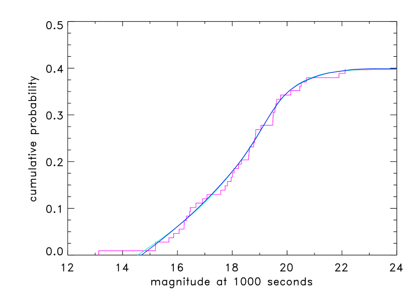
Figure 5.— The cumulative distribution of detected GRB optical afterglows. The violet “staircase” line shows the experimentally observed distribution. The least square estimates are shown in red, green, cyan and blue, corresponding respectively to 4, 5, 6 and 7 degrees of freedom of the b-spline representation.

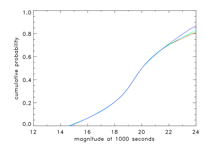
Figure 6.— The intrinsic cumulative GRB apparent optical afterglow distribution. The colors, red, green, cyan and blue, correspond respectively to b-spline curves with 4, 5, 6 and 7 degrees of freedom. Crudely speaking, 71% of all GRB afterglows have $m_{R}<22.1$ at $t_{obs}=1000~{}s$, the dimmest GRB optically detected.

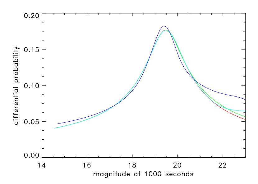
Figure 7.— The differential GRB apparent optical afterglow distribution. The colors, red, green, cyan and blue, correspond respectively to b-spline curves with 4, 5, 6 and 7 degrees of freedom. The peak at $m_{det}\approx 19.5$ seems to be an unavoidable feature.

References

- Angelini et al. (2006) Angelini, L., et al. 2006, GCN Circ. No. 4848
- Antonelli et al. (2006) Antonelli, L. A., et al. 2006, A&A, 456, 509
- Berger et al. (2005) Berger, E., Mulchaey, J., Morrell, N., & Krzeminski, W. 2005, GCN Circ. No. 3283
- Bersier et al. (2003) Bersier, D., et al. 2003, ApJ, 584, L43
- Bikmaev et al. (2005) Bikmaev, I., et al. 2005, GCN Circ. No. 3831
- Bikmaev et al. (2006) Bikmaev, I., et al. 2006, GCN Circ. No. 4652
- Boyd et al. (2005a) Boyd, P., et al. 2005, GCN Circ. No. 4096
- Boyd et al. (2005b) Boyd, P., et al. 2005, GCN Circ. No. 3230
- Boyd et al. (2006) Boyd, P., Weigand, R. E., Holland, S. T., & Blustin, A. 2006, GCN Circ. No. 4958
- Breeveld & Moretti (2006) Breeveld, A. & Moretti, A. 2006, GCN Circ. No. 4798
- Brown et al. (2005a) Brown, P. J., Band, D. L., Boyd, P., Norris, J., Hurley, K., & Gehrels, N. 2005, GCN Circ. No. 3759
- Brown et al. (2005b) Brown, P. J., Mineo, T., Chester, M., Angelini, L., Meszaros, P., & Gehrels, N. 2005, GCN Circ. No. 4200
- Burenin et al. (2003) Burenin, R., et al. 2003, GCN Circ. No. 2001
- Cenko & Fox (2005) Cenko, S. B. & Fox, D. B. 2005, GCN Circ. No. 3981
- Cenko et al. (2005) Cenko, S. B., Fox, D. B., Rich, J., Schmidt, B., Christiansen, J., & Berger, E. 2005, GCN Circ. No. 3357
- Cenko et al. (2006a) Cenko, S. B., et al. 2006, ApJ, 652, 490
- Cenko et al. (2006b) Cenko, S. B., Ofek, E. O., & Fox, D. B. 2006, GCN Circ. No. 5048
- Chen et al. (2005) Chen, Y. T., Huang, K. Y., Ip, W. H., Urata, Y., Qiu, Y., & Lou, Y. Q. 2005, GCN Circ. No. 4285
- Chester et al. (2005) Chester, M., Covino, S., Schady, P., & Roming, P. 2005, GCN Circ. No. 3670
- Cobb (2006) Cobb, B. E. 2006, GCN Circ. No. 4872
- Cobb & Bailyn (2005) Cobb, B. E. & Bailyn, C. D. 2005, GCN Circ. No. 3994
- Covino et al. (2003) Covino, S., et al. 2003, A&A, 404, L5
- Cucchiara et al. (2005) Cucchiara, A., Cummings, J., Holland, S., Gronwall, C., Blustin, A., Marshall, F., Smale, A., Cominsky, L., & Gehrels, N. 2005, GCN Circ. No. 3923
- De Pasquale et al. (2006) De Pasquale, M., et al. 2006, MNRAS, 370, 1859
- Eadie et al. (1971) Eadie, W. T., Drijard, D., James, F. E., Roos, M., & Sadoulet, B. 1971. Statistical methods in experimental physics, pp. 268-271. North-Holland Publishing Company, Amsterdam
- Fox et al. (2005) Fox, D. B., Cenko, S. B., & Schmidt, B. P. 2005, GCN Circ. No. 3931
- Fynbo et al. (2001) Fynbo, J. U., et al. Apr, 2001, A&A, 369, 373
- Gendre & Boër (2005) Gendre, B. & Boër, M. 2005, A&A, 430, 465
- Goad et al. (2006) Goad, M. R., et al. 2006, GCN Circ. No. 4985
- Guetta et al. (2007) Guetta, D., et al. 2007, A&A, 461, 95
- Guidorzi et al. (2005a) Guidorzi, C., et al. 2005, GCN Circ. No. 3625
- Guidorzi et al. (2005b) Guidorzi, C., et al. 2005, ApJ, 630, L121
- Guidorzi et al. (2005c) Guidorzi, C., et al. 2005, GCN Circ. No. 4035
- Guidorzi et al. (2006) Guidorzi, C., et al. 2006, GCN Circ. No. 4661
- Guziy et al. (2006) Guziy, S., Velarde, G. G., & Castro-Tirado, A. J. 2006, GCN Circ. No. 4896
- Halpern & Mirabal (2006) Halpern, J. P. & Mirabal, N. 2006, GCN Circ. No. 5086
- Holland et al. (2005a) Holland, S. T., Band, D., Mason, K., Marshall, F., & Gehrels, N. 2005, GCN Circ. No. 4300
- Holland et al. (2005b) Holland, S. T., et al. 2005, GCN Circ. No. 3150
- Huang et al. (2005) Huang, F. Y., Huang, K. Y., Ip, W. H., Urata, Y., Qiu, Y., & Lou, Y. Q. 2005, GCN Circ. No. 4231
- Hurkett et al. (2006) Hurkett, C., Beardmore, A., Godet, O., Kennea, J. A., Krimm, H., Marshall, F., Osborne, J., Palmer, D., & Parsons, A. 2006, GCN Circ. No. 4736
- Hurkett et al. (2005) Hurkett, C., Page, K., Kennea, J., Burrows, D., Blustin, A., Barbier, L., Markwardt, C., Parsons, A., & Gehrels, N. 2005, GCN Circ. No. 3633
- Jakobsson et al. (2004) Jakobsson, P., Hjorth, J., Fynbo, J. P. U., Watson, D., Pedersen, K., Björnsson, G., & Gorosabel, J. 2004, ApJ, 617, L21
- Jakobsson et al. (2006) Jakobsson, P., et al. 2006, A&A, 447, 897
- Jelínek et al. (2006) Jelínek, M., et al. 2006, A&A, 454, L119
- Jelinek et al. (2005) Jelinek, M., Prouza, M., Kubanek, P., Nekola, M., & Hudec, R. 2005, GCN Circ. No. 3854
- Kendall & Stuart (1979) Kendall, M. & Stuart, A. 1979. The advanced theory of statistics: Volume 2: Inference and relationship, pp. 474-476. Charles Griffin & Company Limited, London, 4th edition
- Klose et al. (2003) Klose, S., et al. 2003, ApJ, 592, 1025
- Klotz et al. (2005a) Klotz, A., Boer, M., & Atteia, J. L. 2005, GCN Circ. No. 3403
- Klotz et al. (2005b) Klotz, A., Boer, M., & Atteia, J. L. 2005, GCN Circ. No. 4386
- Klotz et al. (2006a) Klotz, A., Boer, M., & Atteia, J. L. 2006, GCN Circ. No. 4483
- Klotz et al. (2005c) Klotz, A., Boer, M., Atteia, J. L., & Stratta, G. 2005, GCN Circ. No. 3084
- Klotz et al. (2005d) Klotz, A., Boër, M., Atteia, J. L., Stratta, G., Behrend, R., Malacrino, F., & Damerdji, Y. 2005, A&A, 439, L35
- Klotz et al. (2006b) Klotz, A., Gendre, B., Stratta, G., Atteia, J. L., Boër, M., Malacrino, F., Damerdji, Y., & Behrend, R. 2006, A&A, 451, L39
- Koppelman (2006) Koppelman, M. 2006, GCN Circ. No. 4977
- Kosugi et al. (2005) Kosugi, G., Kawai, N., Aoki, K., Hattori, T., Ohta, K., & Yamada, T. 2005, GCN Circ. No. 3263
- Levan et al. (2006) Levan, A., et al. 2006, ApJ, 647, 471
- Li (2006) Li, W. 2006, GCN Circ. No. 4499
- Li et al. (2006) Li, W., Chornock, R., Butler, N., Bloom, J., & Filippenko, A. V. 2006, GCN Circ. No. 5027
- lin et al. (2005) Lin, Z. Y., Huang, K. Y., Ip, W. H., Urata, Y., Qiu, Y., & Lou, Y. Q. 2005, GCN Circ. No. 3593
- Lipunov et al. (2005) Lipunov, V., et al. 2005, GCN Circ. No. 3883
- Malesani et al. (2005) Malesani, D., D’Avanzo, P., Israel, G. L., Piranomonte, S., Chincarini, G., Stella, L., Tagliaferri, G., & Depagne, E. 2005, GCN Circ. No. 3614
- Mangano et al. (2005) Mangano, V., et al. 2005, GCN Circ. No. 3884
- Mangano et al. (2006a) Mangano, V., et al. 2006, GCN Circ. No. 5014
- Mangano et al. (2006b) Mangano, V., et al. 2006, GCN Circ. No. 5006
- Marshall et al. (2006) Marshall, F., Chester, M., & Cummings, J. 2006, GCN Circ. No. 4814
- McGowan et al. (2005a) McGowan, K., Band, D., Brown, P., Gronwall, C., Huckle, H., & Hancock, B. 2005, GCN Circ. No. 3739
- McGowan et al. (2005b) McGowan, K., et al. 2005, GCN Circ. No. 3317
- Monfardini et al. (2005) Monfardini, A., Gomboc, A., Guidorzi, C., Mundell, C. G., Steele, I. A., Mottram, C. J., Carter, D., Smith, R. J., & Bode, M. F. 2005, GCN Circ. No. 3503
- Monfardini et al. (2006a) Monfardini, A., et al. 2006, ApJ, 648, 1125
- Monfardini et al. (2006b) Monfardini, A., et al. 2006, GCN Circ. No. 4630
- Nardini et al. (2006a) Nardini, M., Ghisellini, G., Ghirlanda, G., Tavecchio, F., Firmani, C., & Lazzati, D. 2006, A&A, 451, 821
- Nardini et al. (2006b) Nardini, M., Ghisellini, G., Ghirlanda, G., Tavecchio, F., Firmani, C., & Lazzati, D. 2006, astro-ph 0612486v1
- Nelder (1965) Nelder, R. 1965, Computer Journal, 7, 308
- Norris et al. (2005) Norris, J., et al. 2005, GCN Circ. No. 4061
- Oates et al. (2006) Oates, S. R., et al. 2006, MNRAS, 372, 327
- Pagani et al. (2006) Pagani, C., et al. 2006, ApJ, 645, 1315
- Page et al. (2005) Page, M. J., Ziaeepour, H., Blustin, A. J., Chester, M., Fink, R., & Gehrels, N. 2005, GCN Circ. No. 3859
- Pandey et al. (2006) Pandey, S. B., et al. 2006, A&A, 460, 415
- Pasquale et al. (2006) Pasquale, M. D., et al. 2006, GCN Circ. No. 4455
- Pasquale et al. (2005) Pasquale, M. D., Norris, J., Kennedy, T., Mason, K., & Gehrels, N. 2005, GCN Circ. No. 4028
- Poole et al. (2005a) Poole, T., et al. 2005, GCN Circ. No. 3050
- Poole et al. (2005b) Poole, T., Hurkett, C., Hunsberger, S., Breeveld, A., Boyd, P., Gehrels, N., Mason, K., & Nousek, J. 2005, GCN Circ. No. 3394
- Poole et al. (2005c) Poole, T., Moretti, A., Holland, S. T., Chester, M., Angelini, L., & Gehrels, N. 2005, GCN Circ. No. 3698
- Poole & Boyd (2006) Poole, T. S. & Boyd, P. T. 2006, GCN Circ. No. 4951
- Press et al. (1992) Press, W. H., Teukolsky, S. A., Vetterling, W. T., & Flannery, B. P. 1992. Numerical recipes in c: The art of scientific computing. Cambridge University Press, Cambridge, 2d edition
- Quimby et al. (2003) Quimby, R., McMahon, E., & Murphy, J. 2003, GCN Circ. No. 2298
- Quimby et al. (2006a) Quimby, R., Schaefer, B. E., & Swan, H. 2006, GCN Circ. No. 4782
- Quimby et al. (2006b) Quimby, R. M., et al. 2006, ApJ, 640, 402
- Reichart & Price (2002) Reichart, D. E. & Price, P. A. 2002, ApJ, 565, 174
- Retter et al. (2005a) Retter, A., et al. 2005, GCN Circ. No. 3788
- Retter et al. (2005b) Retter, A., et al. 2005, GCN Circ. No. 3799
- Retter et al. (2005c) Retter, A., Barthelmy, S., Burrows, D., Chester, M., Gehrels, N., Kennea, J., Marshall, F., Palmer, D., & Racusin, J. 2005, GCN Circ. No. 4126
- Rol et al. (2005) Rol, E., Wijers, R. A. M. J., Kouveliotou, C., Kaper, L., & Kaneko, Y. May 2005, ApJ, 624, 868
- Romano et al. (2006) Romano, P., et al. 2006, A&A, 456, 917
- Roming et al. (2005) Roming, P., et al. 2005, GCN Circ. No. 3026
- Rosen et al. (2005) Rosen, S., et al. 2005, GCN Circ. No. 3095
- Rumyantsev et al. (2005) Rumyantsev, V., Biryukov, V., Pozanenko, A., & Ibrahimov, M. 2005, GCN Circ. No. 4087
- Rumyantsev et al. (2003) Rumyantsev, V., Pavlenko, E., Efimov, Y., Antoniuk, K., Antoniuk, O., Primak, N., & Pozanenko, A. 2003, GCN Circ. No. 2005
- Rykoff et al. (2006a) Rykoff, E. S., et al. 2006, ApJ, 638, L5
- Rykoff et al. (2006b) Rykoff, E. S., Schaefer, B. E., Yost, S. A., & Quimby, R. 2006, GCN Circ. No. 5041
- Rykoff et al. (2005a) Rykoff, E. S., et al. 2005, ApJ, 631, L121
- Rykoff et al. (2005b) Rykoff, E. S., Yost, S. A., Rujopakarn, W., Quimby, R., Smith, D. A., & Yuan, F. 2005, GCN Circ. No. 4012
- Rykoff et al. (2005c) Rykoff, E. S., Yost, S. A., & Swan, H. 2005, GCN Circ. No. 3304
- Schady et al. (2005a) Schady, P., Fox, D., Roming, P., Cucchiara, A., Still, M., Holland, S. T., Blustin, A., & Gehrels, N. 2005, GCN Circ. No. 3817
- Schady et al. (2005b) Schady, P., et al. 2005, GCN Circ. No. 3039
- Schady et al. (2006) Schady, P., et al. 2006, ApJ, 643, 276
- Schady et al. (2005c) Schady, P., Sakamoto, T., McGowan, K., Boyd, P., Roming, P., Nousek, J., & Gehrels, N. 2005, GCN Circ. No. 3276
- Schaefer et al. (2006) Schaefer, B. E., Yuan, F., Yost, S. A., & Quimby, R. 2006, GCN Circ. No. 4860
- Schlegel et al. (1998) Schlegel, D. J., Finkbeiner, D. P., & Davis, M. 1998, ApJ, 500, 525
- Sharapov et al. (2006) Sharapov, D., Ibrahimov, M., & Pozanenko, A. 2006, GCN Circ. No. 4925
- Smith (2005) Smith, D. A. 2005, GCN Circ. No. 3056
- Smith et al. (2005) Smith, D. A., Rykoff, E. S., & Yost, S. A. 2005, GCN Circ. No. 3021
- Stanek et al. (2007) Stanek, K. Z., et al. 2007, ApJ, 654, L21
- Stanek et al. (1999) Stanek, K. Z., Garnavich, P. M., Kaluzny, J., Pych, W., & Thompson, I. 1999, ApJ, 522, L39
- Still et al. (2005) Still, M., et al. 2005, ApJ, 635, 1187
- Swan et al. (2006) Swan, H., Akerlof, C., Rykoff, E., Yost, S., & Smith, I. 2006, GCN Circ. No. 4568
- Swan et al. (2007) Swan, H. F., et al. 2007, manuscript in preparation
- Torii (2005a) Torii, K. 2005, GCN Circ. No. 3943
- Torii (2005b) Torii, K. 2005, GCN Circ. No. 4112
- Torii (2006) Torii, K. 2006, GCN Circ. No. 4826
- Tristram et al. (2005a) Tristram, P., Castro-Tirado, A. J., Guziy, S., Postigo, A. d. U., Jelinek, M., Gorosabel, J., & Yock, P. 2005, GCN Circ. No. 3965
- Tristram et al. (2005b) Tristram, P., Jelinek, M., Castro-Tirado, A. J., Postigo, A. d. U., Guziy, S., Gorosabel, J., & Yock, P. 2005, GCN Circ. No. 4055
- van Paradijs et al. (1997) van Paradijs, J., et al. 1997, Nature, 386, 686
- Vergani et al. (2004) Vergani, S. D., Molinari, E., Zerbi, F. M., & Chincarini, G. 2004, A&A, 415, 171
- Wozniak et al. (2005) Wozniak, P., Vestrand, W. T., Wren, J., Evans, S., & White, R. 2005, GCN Circ. No. 3414
- Wren et al. (2005) Wren, J., Vestrand, W. T., White, R., Wozniak, P., & Evans, S. 2005, GCN Circ. No. 4380
- Yanagisawa et al. (2005) Yanagisawa, K., Sakamoto, T., & Kawai, N. 2005, GCN Circ. No. 4418
- Yanagisawa et al. (2006) Yanagisawa, K., Toda, H., & Kawai, N. 2006, GCN Circ. No. 4517
- Yost et al. (2007) Yost, S. A., et al. 2007, ApJ, 657, 925
- Zhai et al. (2006) Zhai, M., Qiu, Y. L., Wei, J. Y., Hu, J. Y., Deng, J. S., Wang, X. F., Huang, K. Y., & Urata, Y. 2006, GCN Circ. No. 5057
- Zharikov et al. (2003) Zharikov, S., Benitez, E., Torrealba, J., & Stepanian, J. 2003, GCN Circ. No. 2022
- Zheng et al. (2006) Zheng, W. K., Zhai, M., Qiu, Y. L., Wei, J. Y., Hu, J. Y., & Deng, J. S. 2006, GCN Circ. No. 4930
- Ziaeepour et al. (2006) Ziaeepour, H., et al. 2006, GCN Circ. No. 4429