Chiral vibrations in the A=135 region

Abstract

Chiral vibrations in the A=135 region are studied in the framework of a RPA plus self-consistent tilted axis cranking formalism. In this model chiral vibrations appear as a precursor towards the static chiral regime. The properties of the RPA phonons are discussed and compared to experimental data. We discuss the limits the chiral region and the transition to the non harmonic regime.

I Introduction

Chirality is an important symmetry in many physical systems. It is a static property of the geometry of molecules with more than four different atoms, which can have left-handed and right-handed enantiomers. In these cases the left- and right-handed geometry is connected by reflection in a plane. In particle physics chirality is a dynamical feature of mass-less particles, which indicates orientation of the intrinsic spin relative to the linear momentum. In a rotating nucleus it arises as a combination of a dynamical property, the angular momentum, with a static property, the reflection symmetric triaxial shape of the nucleus. If the angular momentum vector lays outside any of the three principal planes, there are a left-handed and a right-handed arrangement, which are connected by the time reversal operation. This kind of chirality is manifested as a pair of (almost) degenerate rotational bands with the same parity Fr01 . Pairs of such bands have been seen experimentally in the mass regions A=105, A=135 and A=190 and theoretically described using mean field tilted axis cranking (TAC) models DF00 ; OD04 , two-particle-rotor models FM97 ; SC02 or extensions of the IBA model BV04 ; TA06 .

Chirality appears both in molecules and nuclei as a spontaneously broken symmetry: The many-body Hamiltonian describing these systems is invariant with respect to the chiral operation (space inversion or time reversal, respectively), which has the consequence that the exact eigenfunctions are achiral. However, there exist very good approximate solutions, which are chiral, where the left-handed and right-handed configurations have the same energy. The exact eigenfunctions are odd and even superpositions of these chiral solutions. The energy splitting between these states is given by the interaction matrix element between the two chiral configurations, which is the inverse time for tunneling from one to the other. In most molecules the tunneling time is so long that they stay in one of the enantiomers, and the level splitting is unmeasurable. However, for CH₃NHF the tunneling is rapid. The splitting is in the order of 100 meV, i.e. the tunneling frequency is in the order of 3000 GHz, which is somewhat larger than the average rotational frequency of the molecule at room temperature. For the known nuclear cases, the left-right conversion is always rapid. The observed energy distance between the chiral partners is in the order of 100 keV SK01 , except in very narrow spin regions, where the bands cross. This is comparable with the rotational frequency in the observed spin range.

TAC is a microscopic mean field method that has been shown to very well describe the energy and the intra-band transition rates of the lower of the two chiral partner bands, see e.g. HB01 . However, it gives either one achiral self-consistent solution or two degenerate chiral ones. It can not describe the left-right mode, which is a well known deficiency of the mean field solution when it breaks spontaneously a symmetry (cf. e.g. RS80 ; Fr01 ). In a finite system, as the nucleus, the symmetry breaking develops in a gradual way. First a precursor appears as a slow vibration around the symmetric configuration. Becoming increasingly anharmonic, the vibration changes into tunneling between two asymmetric configurations, which is progressively inhibited.

In order to describe the splitting between the two bands one has to go beyond the mean field approximation. So far this has only be done in the framework of two-particle-core coupling models FM97 ; SC02 ; BV04 ; TA06 . These studies show a development from chiral vibrations toward tunneling between static left- and right-handed configurations with increasing angular momentum. Although the quantal nature allow the core-particle models to account well for this aspect of symmetry breaking, they are based on several assumptions the validity of which is not assured. Examples are: Rigid shape and irrotational-flow moments of inertia for a triaxial rotor core FM97 ; SC02 , which are not consistent with microscopic cranking calculations TA06 , the application of the IBA core, and the IBAFF coupling scheme BV04 ; TA06 . A microscopic treatment starting from the TAC mean field seems important for a better understanding of nuclear chirality. Obviously the transition from chiral vibrations to chiral rotation involves large amplitude collective motion, a treatment of which goes beyond the scope of this paper. However the regime of chiral vibration can be treated by the Random Phase Approximation (RPA) approach as long as the energy splitting between the bands is large enough for the assumption of a harmonic vibration remaining reasonable. As the energy splitting decreases the anharmonic effects will become more important until the transition point where the RPA energy becomes zero and the TAC mean field becomes chiral. The present paper is devoted to a study of the spin range before the transition point where the RPA approximation will allow us investigating the chiral vibrations and provide insight into the nature of nuclear chirality.

In the static chiral picture one would expect the two bands to have very similar electromagnetic transition rates. Recent experiments have shown different intra-band transition rates in the two chiral partner bands in ¹³⁴Pr TA06 ; PH06 while the bands in ¹²⁸Cs GS06 and ¹³⁵Nd MA07 have similar transition rates. The different transition rates in ¹³⁴Pr have been interpreted as being due to coupling of shape degrees of freedom to the orientation degree of freedom TA06 or even that the bands are not chiral partner bands at all PH06 .

Chiral pairs of rotational bands have mainly been suggested for nuclei with odd proton and odd neutron number. In the A=135 region, they are build on the $\pi h_{11/2}\otimes\nu h_{11/2}^{-1}$ configuration. Candidate bands have been seen in the odd-odd nuclei ^126-132Cs, ^130-134La, ^132-134Pr, ¹³⁶Pm and ^138-140Eu. In this work we focus on the N=75 isotone chain and the Z=57 isotope chain which represent the central part of this region. We have performed calculations in the framework of tilted axis cranking (TAC) and random phase approximation (RPA) for the twin bands in the N=75 isotones and the Z=57 isotopes built on the $\pi h_{11/2}\otimes\nu h_{11/2}^{-1}$ configuration. Examples for chiral partner bands exist also in odd-even nuclei ZG03 ; MA07 . The case of ¹³⁵Nd has been studied in MA07 by means of the method presented in this paper. In principle, chiral partner bands should also exist in even-even nuclei build on two-particle two-hole like configurations. For these and even more complex configurations our method can be directly applied. We describe the formalism in section II. The results for the energy, amplitudes and transition rates are presented in section III. An analysis of the structure of the phonons is given in section IV, where it will be demonstrated that for most of the cases the chiral character prevails, i.e. the coupling to the shape degrees of freedom is weak.

II Formalism

Most earlier TAC calculations for chiral bands have used the Strutinsky shell correction method for calculating energies and band properties (c.f. the SCTAC model  Fr00 ). In this paper we present selfconsistent RPA calculations which are founded on the TAC plus RPA with a residual quadrupole-quadrupole (QQ) interaction. The corresponding Hamiltonian $\hat{H}$ which similar to the one of the PQTAC model Fr00 is given by

$$\hat{H} = \sum_{\tau=\pm 1}[\,\,\hat{h}^{\circ}_{\tau}-\Delta_{\tau}(\hat{P}^{\dagger}_{\tau}+\hat{P}_{\tau})-\lambda_{\tau}\hat{N}_{\tau}\,\,]-\boldsymbol{\omega}\cdot\boldsymbol{\hat{J}}-\frac{\kappa_{{}_{0}}}{2}\sum_{m=-2,2}(-1)^{m}\hat{Q}^{(BK)}_{m}\hat{Q}^{(BK)}_{-m}.$$ (1)

The first part $\hat{h}^{\circ}_{\tau}$ is the spherical single particle term of the Hybrid TAC model DF00 which on one hand takes advantage of using single particle energies of the spherical Woods-Saxon model and on second hand it uses the same oscillator basis with the spherical quantum numbers $\{n,l,j,m\}$ as applied here. The isospin index $\tau=\pm 1$ distinguishes the neutron and proton contributions, respectively, in the Hamiltonian. The second term $\Delta_{\tau}(\hat{P}^{\dagger}_{\tau}+\hat{P}_{\tau})$ means a pair field where $\hat{P}^{\dagger}_{\tau}$ and $\hat{P}_{\tau}$ are the familiar monopole pair operators. The gap parameters $\Delta_{\tau}$ are 80% of the odd-even mass differences to the respective neighboring nuclides. The third term $\lambda_{\tau}\hat{N}_{\tau}$ implying the particle number operators $\hat{N}_{\tau}$ is introduced as usual for saving in average the numbers of protons and neutrons, Z and N, respectively by appropriate choice of the Fermi energy $\lambda_{\tau}$. The forth term $-\,\boldsymbol{\omega}\cdot\boldsymbol{\hat{J}}$ in Eq.(1) is a 3d-cranking energy term. Therein the vector $\boldsymbol{\omega}=(\omega_{1},\omega_{2},\omega_{3})$ defines the angular frequency $\omega=|\boldsymbol{\omega}|$ and the direction of the cranking axis (cf. Eq. (II)). The operator $\boldsymbol{\hat{J}}$ means the total angular momentum operator.

The last contribution in the Hamiltonian $\hat{H}$, Eq. (1) is an isoscalar QQ interaction with the strength parameter $\kappa_{{}_{0}}$. We adopt the modified quadrupole operators $\hat{Q}^{(BK)}_{m}$ of the collective model by Baranger and Kumar (BK) BK68

$$\hat{Q}^{(BK)}_{m} = \hat{Q}^{(BK)}_{m}(\tau=+1)+\hat{Q}^{(BK)}_{m}(\tau=-1)$$ (2)

$$\text{where}\quad\quad\hat{Q}^{(BK)}_{m}(\tau) = \left(\frac{n_{\rm low}-B}{\hat{n}-B}\right)\left(\frac{2A_{\tau}}{A}\right)^{1/3}r^{2}Y_{2m}(\tau),\quad\quad m=0,\pm 1,\pm 2$$

The operator $\hat{n}$ counts the number of oscillator quanta $n$, i.e. $\hat{n}\,|nljm\rangle=n\,|nljm\rangle$.

Compared to the usual isoscalar quadrupole operator $\hat{Q}_{m}=r^{2}Y_{2m}(\tau=+1)+r^{2}Y_{2m}(\tau=-1)$ the operator $Q^{(KB)}_{m}$ in Eq. (2) contains additionally quenching factors which depend on the isospin, the mass number $A$, the oscillator shell quantum number $n$ and a stiffness parameter $B$. The oscillator basis of our calculations includes all substates of the two oscillator shells $n=n_{low}=4$ and $n=5$. The value of the parameter $B$ is chosen to approximately reproducing potential energy surfaces obtained by the Strutinsky correction method Fr00 . Setting the parameter $B=0.5$ gives a similar prolate-oblate mass difference and $\gamma$-softness as SCTAC calculations in this mass region. In other mass regions a different value of $B$ may be needed. The strength parameters $\kappa_{{}_{0}}$ for the considered nuclides are listed in table 1. They are adjusted to fulfill the self-consistency conditions (c.f. Eq. (II)) at the minimum of the potential energy surfaces obtained by the Strutinsky shell correction method. This choice ensures that the two spurious RPA solutions appear at the predefined energies $E_{{}_{RPA}}=0$ and $E_{{}_{RPA}}=\hbar\omega$. In order to simplify the notation we will leave out in what follows the suffix $(BK)$ of the operator $Q^{(BK)}_{m}$ keeping in mind that we are working in this paper with the BK modification.

Table 1: Quadrupole force strength $\kappa_{{}_{0}}$.

	$\kappa_{{}_{0}}$ (MeV fm-4)
130Cs	0.00354
132La	0.00343
134Pr	0.00329
136Pm	0.00333
138Eu	0.00337
140Tb	0.00328
130La	0.00359
134La	0.00319

The first step of the calculation is the search for self-consistent (s.c.) TAC solutions, which for a fixed strength $\kappa_{{}_{0}}$ and within the considered frequency range $\omega$ = 0.1 - 0.4 MeV correspond to a tilted cranking solution. The general scheme of these calculations has been described in Ref. Fr00 . The deformed potential $v$ produced by the mean field contribution from the QQ interaction has the form

$$v=v(q_{{}_{0}},q_{{}_{2}})=\kappa_{{}_{0}}q_{{}_{0}}\hat{Q}_{{}_{0}}+\kappa_{{}_{0}}q_{{}_{2}}(\hat{Q}_{{}_{2}}+\hat{Q}_{{}_{-2}}),$$ (3)

where $q_{{}_{0}}$ and $q_{{}_{2}}$ are defined by the expectation values

$$\langle\hat{Q}_{{}_{0}}\rangle = q_{{}_{0}}$$

$$\langle\hat{Q}_{{}_{2}}\rangle = \langle\hat{Q}_{{}_{-2}}\rangle=q_{{}_{2}},$$ (4)

and $\rangle$ is the short hand notation for the TAC solution $|TAC\rangle$ for the selected configuration. The absence of the components $\hat{Q}_{{}_{\pm 1}}$ in the deformed potential (3) ensures that the condition $\langle\hat{Q}_{{}_{1}}\rangle=\langle\hat{Q}_{{}_{-1}}\rangle=0$ is satisfied and, therefore, one stays in the principal axes (P-) system of the uniformly rotating ellipsoidal potential. This holds generally, i.e. also for mean field states with a tilted cranking axis. Eqs.(II) represent the two selfconsistency conditions for the nuclear shape. Actually we are using the deformation parameters $(\varepsilon,\gamma)$ of the modified oscillator model Nilsson-Ragnarsson . Then the s.c. conditions take the form

$$\kappa_{{}_{0}}\langle\hat{Q}_{{}_{0}}\rangle=\kappa_{{}_{0}}q_{{}_{0}}(\varepsilon,\gamma) = \,\,\hbar\omega_{{}_{0}}\,2/3\,\varepsilon\cos{\gamma}$$

$$\kappa_{{}_{0}}\langle\hat{Q}_{{}_{2}}\rangle=\kappa_{{}_{0}}q_{{}_{2}}(\varepsilon,\gamma) = -\hbar\omega_{{}_{0}}\,2/3\,\varepsilon\sin{\gamma}/\sqrt{2}.$$ (5)

where $\hbar\omega_{{}_{0}}=41A^{-1/3}$ is the usual oscillator frequency.

The P-components of the rotational frequency vector $\boldsymbol{\omega}$ in Eq.(1) are expressed by the spherical angles $(\vartheta,\varphi)$:

$$\omega_{{}_{1}}~{} = ~{}\omega~{}\sin\vartheta\cos\varphi$$

$$\omega_{{}_{2}}~{} = ~{}\omega~{}\sin\vartheta\sin\varphi$$ (6)

$$\omega_{{}_{3}}~{} = ~{}\omega~{}\cos\vartheta~{}.$$

The SCTAC model includes the selfconsistency with respect to the spin orientation, i.e. the stability of the angular momentum vector $\boldsymbol{J}=\langle\boldsymbol{\hat{J}}\rangle$. The s.c. orientation of the angular momentum $\boldsymbol{J}$ is determined by the parallel condition $\boldsymbol{\omega}\|\boldsymbol{J}$  Fr00 which fixes the angles $(\vartheta,\varphi)$ in Eq.(II) for given frequency $\omega$. Because the vector $\boldsymbol{J}$ is a constant of motion in the laboratory (L-) system, it is a still-standing vector about which the deformed nucleus is uniformly rotating. Hence we can chose the laboratory $z$-axis along this direction which fixes the transformation from the P- to the L-system needed below.

In our TAC calculations for the A=135 region, chiral solutions appear as a transient phenomenon. With increasing frequency, the angular momentum vector moves from the principal axis plane $\varphi=0$ spanned by the 1- (short) and 3- (long) axis to the principal plane $|\varphi|=90^{\circ}$ spanned by the 2- (intermediate) and 3-(long) axis  DF00 . This can be seen e.g. in Tab.2 for the case ¹³⁶Pm. The RPA calculations are based on the regimes where the TAC angular momentum lays within one of these principal planes. Then the excited chiral partner band can be described in RPA as a chiral vibration, which is a periodic motion of the orientation of the deformed potential relative to angular momentum vector $\boldsymbol{J}$, i.e. a vibration of the angles $\vartheta$ and $\varphi$ about their equilibrium values. There are two critical frequencies. The first one is associated with the transition of the TAC mean field solution at $\varphi=0$ into the static chiral regime, and the second one is associated with the transition out of chiral regime at $|\varphi|=90^{\circ}$. These transitions of the mean field are accompanied by instabilities of the RPA, where the energy of the lowest RPA phonon becomes zero thus indicating that the RPA is not applicable beyond the critical frequency.

When the TAC solution has reached the static chiral regime $0<|\varphi|<90^{\circ}$ our present approach gives zero energy splitting between the two chiral configurations with $\varphi=\pm|\varphi|$. However, higher order terms in our Hamiltonian would give rise to tunneling between the left-handed and the right-handed solution which causes an energy splitting between the two bands in this region too.

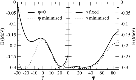
Figure 1: Potential energy in the rotating frame for ¹³⁴Pr at $\omega=0.4$ MeV/$\hbar$. The two solid curves are calculated with $\gamma$ or $\varphi$ (in degrees) fixed while the dotted curve is calculated with a full minimization.

Figure 1 shows the TAC energy in the rotating frame, spanned by the three principal axes of the triaxial density distribution, as a function of the tilt angle $\varphi$ and the triaxial deformation parameter $\gamma$. The calculation is done for the two quasi particle (2qp) configuration $\pi h_{11/2}\otimes\nu h_{11/2}$ in ¹³⁴Pr at $\omega=0.4$ MeV. The energy surface is rather shallow especially in the $\varphi$ direction. When we allow for the full minimization in the orientation degrees of freedom the surface becomes symmetric in $\pm\gamma$, because the change of sign is equivalent with a reorientation of the axes. It is therefore enough to consider $\gamma>0$ only.

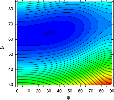
Figure 2: (Color online) Potential energy surface in the rotating frame for the 2qp configuration $\pi h_{11/2}\otimes\nu h_{11/2}$ in ¹³⁴Pr at $\omega=0.4$ MeV/$\hbar$ as a function of the tilt angles $\vartheta$ and $\varphi$ (in degrees) with constant deformation. The equipotential lines are separated by 25 keV. Darker color represent lower energy.

Table 2: Equilibrium values of the deformation parameters $\varepsilon$,$\gamma$, the tilt angles $\theta,\varphi$ and the lowest RPA phonon energy $\hbar\Omega$ as a function of the cranking frequency $\omega$.

Nuclid	$\omega$(MeV/$\hbar$)	$\varepsilon$	$\gamma$(deg)	$\vartheta$(deg)	$\varphi$(deg)	$\Omega$(MeV/$\hbar$)
130Cs	0.20	0.19	33	59	0	0.30
	0.25	0.19	33	59	0	0.27
	0.30	0.19	32	59	0	0.21
	0.35	0.19	31	60	0	0.12
	0.40	0.19	31	60	19	-
	0.45	0.19	29	61	34	-
132La	0.20	0.21	26	59	0	0.33
	0.25	0.21	26	60	0	0.30
	0.30	0.21	26	61	0	0.26
	0.35	0.21	25	62	0	0.19
	0.40	0.21	24	63	0	0.09
	0.45	0.21	22	64	24	-
134Pr	0.10	0.21	24	57	0	0.30
	0.15	0.21	24	58	0	0.32
	0.20	0.21	24	59	0	0.31
	0.25	0.21	24	60	0	0.28
	0.30	0.21	23	61	0	0.21
	0.35	0.21	22	61	0	0.11
	0.40	0.21	22	64	32	-
136Pm	0.10	0.24	24	50	0	0.14
	0.15	0.24	24	50	0	0.09
	0.20	0.24	24	55	20	-
	0.25	0.24	24	58	38	-
	0.30	0.24	24	62	52	-
	0.35	0.25	24	66	77	-
	0.40	0.25	24	69	90	0.15
	0.45	0.25	21	72	90	0.33
	0.50	0.25	19	75	90	0.42
138Eu	0.05	0.30	21	39	22	-
	0.10	0.29	21	47	90	0.07
	0.15	0.29	21	54	90	0.14
	0.20	0.29	22	58	90	0.20
	0.25	0.29	22	61	90	0.27
	0.30	0.29	22	63	90	0.34
	0.35	0.29	22	65	90	0.40
	0.40	0.29	22	67	90	0.46
140Tb	0.20	0.29	23	53	90	0.27
	0.25	0.29	24	57	90	0.35
	0.30	0.29	25	60	90	0.43
	0.35	0.28	25	64	90	0.50
	0.40	0.28	26	67	90	0.58
130La	0.10	0.26	9	61	0	0.38
	0.15	0.25	12	63	0	0.43
	0.20	0.25	13	65	0	0.48
	0.25	0.25	11	66	0	0.53
	0.30	0.25	9	68	0	0.59
	0.35	0.26	8	69	0	0.66
134La	0.10	0.15	38	51	0	0.32
	0.15	0.15	37	52	0	0.42
	0.20	0.15	36	52	0	0.43
	0.25	0.15	35	52	0	0.35
	0.30	0.15	35	52	0	0.27
	0.35	0.15	34	52	0	0.19
	0.40	0.15	33	53	0	0.10
	0.45	0.15	33	53	55	-

Figure 2 shows the potential energy surface in the rotating frame (total routhian) as a function of both angles $\vartheta$ and $\varphi$. One can see the very soft nature of the potential in the $\varphi$ direction.

The RPA accounts for the harmonic excitations above the mean field minimum. It gives an adequate description as long as we are in the chiral vibrational regime well before the transition to static chirality or after returning to the former regime. The transition point corresponds to the rotational frequency where the RPA excitation energy goes to zero. After solving the s.c. mean field problem the Hamiltonian (1) is expressed in terms of the quasiparticle creation (annihilation) operators $\hat{\alpha}_{i}^{\dagger}(\hat{\alpha}_{i})$, and it takes the form

$$\hat{H}=\hat{h}_{\rm mf}+\hat{H}_{\rm res},$$ (7)

where $\hat{h}_{\rm mf}$ is the diagonal mean field Hamiltonian

$$\hat{h}_{\rm mf}=E_{\rm mf}+\sum_{i}e_{i}\hat{\alpha}_{i}^{\dagger}\hat{\alpha}_{i},$$ (8)

and $\hat{H}_{\rm res}$ is the residual QQ interaction. We make use of the quasi-boson approximation $\hat{b}_{\mu}^{\dagger}=\hat{\alpha}_{i}^{\dagger}\hat{\alpha}_{j}^{\dagger}$, where the $\hat{b}_{\mu}^{\dagger}$ are treated as exact bosons, and introduce the combined index $\mu\equiv\{i>j,\tau\}$. The Hamiltonian $\hat{H}$ is rewritten in RPA order by only keeping terms up to second order in the boson operators RS80 , i.e.

$$\hat{H}_{\rm RPA}=E_{\rm mf}+\sum_{\mu,\nu}A_{\mu\nu}\hat{b}_{\mu}^{\dagger}\hat{b}_{\nu}+\frac{1}{2}\sum_{\mu,\nu}\left(B_{\mu\nu}\hat{b}_{\mu}^{\dagger}\hat{b}_{\nu}^{\dagger}+{\rm h.c.}\right).$$ (9)

The matrices ${\bf A}$ and ${\bf B}$ are real and symmetric,

$$A_{\mu\nu} = \delta_{\mu\nu}E_{\mu}-\kappa_{{}_{0}}\sum_{m=-2}^{2}\,q_{\mu}^{m}{q_{\nu}^{m}}^{*},$$

$$B_{\mu\nu} = -\kappa_{{}_{0}}\sum_{m=-2}^{2}\,q_{\mu}^{m}{q_{\nu}^{m}}^{*},$$ (10)

where $q_{\mu}^{m}=\langle\hat{b}_{\mu}\hat{Q}_{m}\rangle$ are the quadrupole matrix elements in quasiboson representation RS80 and $E_{\mu}=e_{i}+e_{j}$ are the 2qp energies. The quadrupole operators $\hat{Q}_{m}$ take the form

$$\hat{Q}_{m} = \sum_{\mu}(q_{\mu}^{m}\hat{b}_{\mu}^{\dagger}+{q_{\mu}^{m}}^{*}\hat{b}_{\mu}).$$ (11)

Note, the sum runs also over $\tau=\pm 1$. We solve the RPA equation

$$\left[\hat{H}_{\rm RPA},\;\,\hat{O}^{\dagger}_{\lambda}\right]=E_{{}_{RPA}}^{\lambda}\hat{O}^{\dagger}_{\lambda},$$ (12)

using the strength function method of RS80 ; KN86 . The RPA eigenmode operators $\hat{O}^{\dagger}_{\lambda}$ are

$$\hat{O}^{\dagger}_{\lambda}=\sum_{\mu}(X^{\lambda}_{\mu}\hat{b}_{\mu}^{\dagger}-Y^{\lambda}_{\mu}\hat{b}_{\mu}),$$ (13)

where the RPA amplitudes $X^{\lambda}_{\mu}$ and $Y^{\lambda}_{\mu}$ are obtained by solving the standard set of linear equations resulting from Eq. (12) together with the normalization condition

$$\left[\hat{O}_{\lambda},\;\,\hat{O}^{\dagger}_{\lambda^{\prime}}\right]=\sum_{\mu}(X^{\lambda}_{\mu}X^{\lambda^{\prime}}_{\mu}-Y^{\lambda}_{\mu}Y^{\lambda^{\prime}}_{\mu})=\delta_{\lambda\lambda^{\prime}}.$$ (14)

Since we use a separable force, this set of linear equations is strongly simplified KN86 .

As mentioned above there are two rotational spurious solutions in the RPA spectrum. One at zero energy $E_{{}_{RPA}}=0$ induced by the angular momentum operator in the L-frame, $\hat{J}_{z}$, and one at the rotational energy $E_{{}_{RPA}}=\hbar\omega$ induced by the corresponding step operator $\hat{J}_{+}=\hat{J}_{x}+i\hat{J}_{y}$. Numerically the spurious solutions decouple from the physical RPA solutions in a stable manner if the mean field problem is solved accurately enough. In the discussion below we will only refer to the physical RPA solutions. They are in all cases well decoupled from the spurious solutions in our numerical procedure. The RPA phonon energy gives the energy splitting between the zero-phonon lower band and the excited one-phonon band at a given rotational frequency $\omega$. From the calculated RPA amplitudes we derive the inter-band transition rates using the method of KN86 . Since the RPA does not give any contribution to the intra-band transition rates, we use the TAC results Fr00 for those.

II.1 Energies

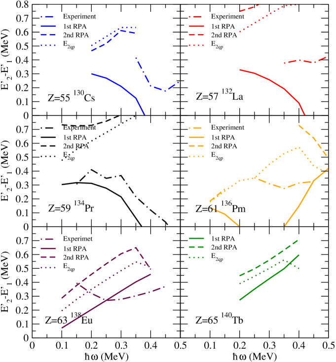
Figure 3: (Color online) Energy differences in the rotating frame between the two chiral partner bands in the N=75 isotone chain. RPA results are compared with experimental data KS03 ; SC02 ; TA06 ; HR01 ; HB01 . We also plot the second RPA phonon energy and the 2qp energy, $E_{2qp}$. The experimental values show the difference between the experimental routhians of the two bands at grid points of $\hbar\omega$ that were calculated by interpolation.

III Results

Below we discuss the results of the TAC + RPA calculations for the N=75 isotones and the Z=57 isotopes. The limits of the studied region are chosen by the following consideration. For lower Z or larger N we approach the shell closing where the deformation disappears. For smaller N the triaxiality disappears. For larger Z one approaches the proton drip line, where very little high spin data are available.

First we solved the selfconsistent TAC problem using the Hamiltonian in Eq. (1) for the 2qp configuration $\pi h_{11/2}\otimes\nu h_{11/2}$. The resulting s.c. values $\varepsilon,\gamma,\vartheta$ and $\varphi$ are summarized in table 2. For N=75, the neutron chemical potential is located in the upper part of the $h_{11/2}$ shell, and the quasi neutron has hole character. For Z=57, the proton chemical potential is located at the bottom of the $h_{11/2}$ shell, and the quasi-proton has particle character. Along the N=75 isotone chain, the proton chemical potential approaches the middle of the of the $h_{11/2}$ shell at Z=65. The change of the quasi proton is reflected by the TAC solution. For low Z and low $\omega$, the energy minimum is at $\varphi=0$, because the particle - like quasi proton aligns with the short axis and the hole - like quasi neutron with the long axis. The two axes define the short - long plane $\varphi=0$. With increasing $\omega$ the intermediate axis, which has a larger moment of inertia, becomes progressively favored until the $\varphi=0$ minimum becomes unstable and static chirality sets in Fr01 ; DF00 ; OD04 ; FM97 . The preference of the short axis over the intermediate one becomes attenuated when the quasi proton loses its particle character with increasing Z. As a consequence, the minimum moves to $\varphi=90^{o}$ into the intermediate-long plane. For Z=65 the $\varphi=90^{o}$ minimum is stable. It is very shallow for Z=63. In these cases the minimum becomes deeper with increasing $\omega$. The Z=61 case is in between. The $\varphi=0$ minimum is very shallow. Static chirality sets in at the relatively low frequency of $\hbar\omega=0.20$ MeV. The chiral minimum is very weak, such that $\varphi=90^{o}$ becomes the location of the minimum for $\hbar\omega\geq 0.40$MeV

In Figs. 3 and 4 the energy of the lowest RPA phonon is compared with the experimental energy splitting between the chiral bands. For reference we also plot the energy of the lowest 2qp excitation (relative to the $\pi h_{11/2}\otimes\nu h_{11/2}$ TAC configuration), as well as the energy of the second physical RPA phonon. In the lighter nuclides the energy of the lowest RPA phonon is substantially smaller than the 2qp excitation energy and the energy of the second RPA phonon. In the heavier nuclides the difference is smaller. For the lowest phonon being a well developed collective excitation it must have a substantially smaller energy than the next excitations. When the lowest phonon sits in a region where other excitations are located the collective strength will become fragmented, and the observed bands will be much like 2qp excitations.

Figure 3 shows the results for the N=75 isotones. The RPA results reflect the properties of the TAC mean field solutions. In the low-Z part of the A=135 region the TAC energy minimum sits at $\varphi=0$ at low spin. As we move towards larger Z the minimum moves over to $\varphi=90^{\circ}$. With increasing $\omega$, $\varphi=90^{\circ}$ is preferred, because the intermediate axis has the largest moment of inertia. In the lighter systems, where the TAC solutions have $\varphi=0$, the phonon energy decreases with spin, reaching zero at the critical frequency indicating the onset of static chirality ($\varphi>0$). In the heavier systems, where the TAC solutions have $\varphi=90^{\circ}$ already at the band head, the phonon energy increases with increasing angular momentum. ¹³⁶Pm is the limiting case where we have a chiral vibration around $\varphi=0$ and decreasing phonon energy at low spin, that goes to a static chiral regime with $0<\varphi<90^{\circ}$, and finally a second chiral vibration around $\varphi=90^{\circ}$ and increasing phonon energy. Comparing with experiment, ¹³⁰Cs, ¹³⁴Pr, ¹³⁸Eu have the right trend and magnitude of the energy splitting. ¹³²La, ¹³⁶Pm have a much more constant energy splitting in the experiment than obtained by the RPA calculations.

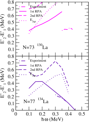
Figure 4: (Color online) Energy differences in the rotating frame between the two chiral partner bands in Z=57 isotopes. RPA results are compared with experimental data KS01 ; BB01 . We also plot the second RPA phonon energy and the 2qp energy, $E_{2qp}$.

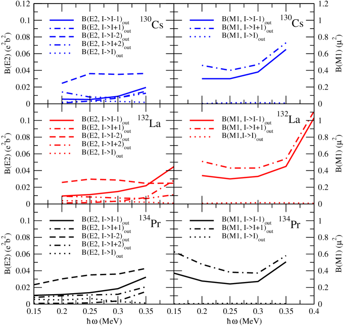
Figure 5: The RPA inter-band transition rates in ¹³⁰Cs, ¹³²La and ¹³⁴Pr.

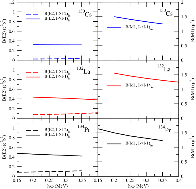
Figure 6: The TAC intra-band transition rates in ¹³⁰Cs, ¹³²La and ¹³⁴Pr.

The inter-band M1 transitions are much stronger in the lighter N=75 isotopes where the B(M1) values are typically around 1/3 of the intra-band values. In the heavier N=75 isotopes as well as in ¹³⁴La the inter-band B(M1) are weak.

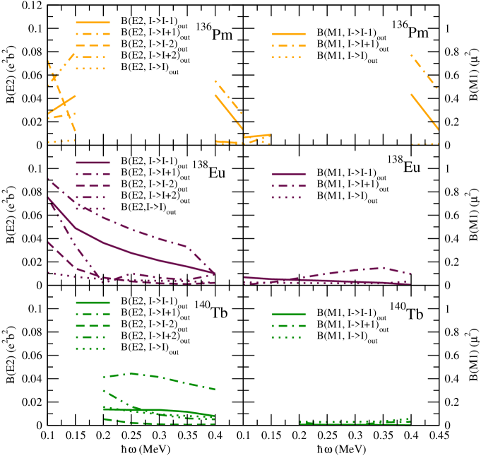
Figure 7: The RPA inter-band transition rates in ¹³⁶Pm, ¹³⁸Eu and ¹⁴⁰Tb.

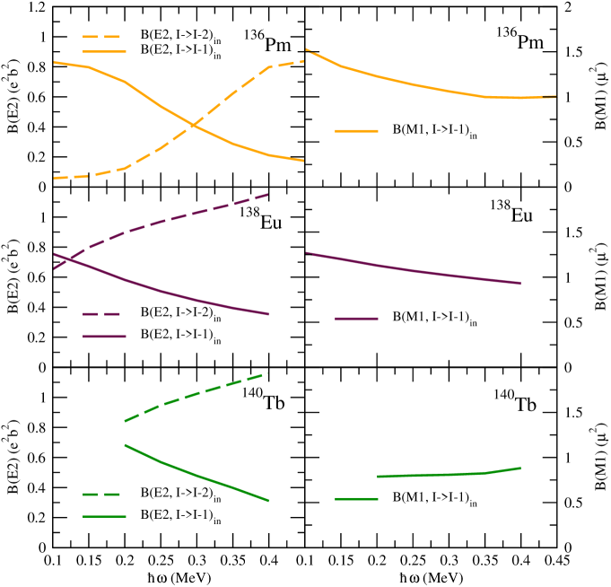
Figure 8: The TAC intra-band transition rates in ¹³⁶Pm, ¹³⁸Eu and ¹⁴⁰Tb.

Figure 4 show the results for the Z=57 isotopes. The magnitude of the energy splitting is reproduced but there is a problem with the frequency trend in ¹³²La. In experiment ¹³²La looks similar to ¹³⁰La while in the calculations it looks more like ¹³⁴La.

Our TAC+RPA calculations give the correct energy splitting away from the region where the RPA energy approaches zero, which is where we can expect the RPA to work well. However, spin dependence is not always well reproduced. The RPA phonon energy tends to approach zero faster and more often than in experiment, which indicates that anharmonic effects are needed to understand the data. The RPA phonon energy is generally increasing or decreasing with rotational frequency. The experimental energy splitting, on the other hand, does not change much with $\omega$ in some cases, which seem to appear predominantly in the frequency regions where the TAC gives static chirality, $0<\varphi<90^{\circ}$, i.e. TAC + RPA predicts zero splitting. The constant energy splitting in these regions should be attributed to the tunneling between the left- and right-handed solutions. Its relatively large value of about $300$ keV indicates strong mixing between the two chiral configurations, which is consistent with the flat potential in $\varphi$ direction in Fig. 2 and our analysis of the composition of the RPA phonon wave function discussed in section IV below. In ¹³⁴Pr the two bands cross over in experiment. In ¹³⁰Cs and ¹³⁵Nd (not shown here, see MA07 ) one sees in experiment an avoided crossing with some interaction. In all three cases, the crossing frequency correlates with the frequency where the phonon energy goes to zero. At moment, it remains unclear why these nuclei are different from ¹³²La and ¹³⁶Pm with a nearly frequency-independent energy difference between the bands. To understand this phenomenon further it is clearly necessary to take into account large amplitude anharmonic effects, which will be done in a forthcoming publication ADF11 .

III.1 Transition rates

In addition to the energy splitting, the RPA also provides the transition rates between the two chiral partner bands which are connected by E2 and M1 radiation with spin differences $\Delta I=0,\pm 1,\pm 2$ . In accordance with the RPA the transition amplitudes are calculated with the multipole operators $\hat{\cal M}_{k}(\lambda;P)$ in the P-system where $\lambda$ defines the multipole order and $k$ the 3-component of the transition. In detail the transition operators are given by

$$\hat{\cal M}_{k}(E2;L) = e_{p}r_{p}^{2}{Y}_{2k}(p)+e_{n}r_{n}^{2}{Y}_{k}(n),\qquad\qquad\qquad k=0,\pm 1,\pm 2$$ (15)

$$\hat{\cal M}_{k}(M1;L) = \frac{3}{4\pi}g^{(l)}_{p}\hat{l}_{1k}(p)+g^{(s)}_{p}\hat{s}_{1k}(p)+g^{(s)}_{n}\hat{s}_{1k}(n),\quad\quad k=0,\pm 1$$ (16)

The effective charges for the E2 are $e_{p}=1+Z/A$ for protons and $e_{n}=Z/A$ for neutrons. The orbital g-factor for M1 is $g^{(l)}_{p}=1\mu_{N}$ for protons and 0 for neutrons. The spin g-factors $g^{(s)}_{p}$ and $g^{(s)}_{n}$ are 0.7 times the values for the free proton or neutron. The above multipole operators are treated by boson expansion in linear order only. Finally we have to remember that the radition is observed in the laboratory system which is taken into account by rotating $\hat{\cal M}_{k}(\lambda;P)$ from the P- to the L-frame:

$$\hat{\cal M}_{m}(\lambda;L)=\sum_{k}D^{\lambda}_{km}(\varphi,-\vartheta,0)\hat{\cal M}_{k}(\lambda;P).$$ (17)

The expression applies to the different planar TAC solution corresponding to $\varphi=0$, i.e that angular momentum vector lies in the plane spanned by the long and short axes, and to $\varphi=90^{o}$, i.e that angular momentum vector lies in the plane spanned by the long and intermediate axes, which gives the additonal phase factor $e^{-ik\frac{\pi}{2}}$ in the sum.

The component $m$ determines the actual spin difference of the transition $I\to I-m$. Hence we obtain the reduced transition probabilities for the inter-band transitions

$$B(E2,I\rightarrow I-m)=\left|\left<1\left|\hat{\cal M}_{m}(E2;L)\right|0\right>\right|^{2}\quad\text{and }\quad B(M1,I\rightarrow I-m)=\left|\left<1\left|\hat{\cal M}_{m}(M1;L)\right|0\right>\right|^{2}$$ (18)

where $\left|0\right>$ is the RPA ground state and $\left|1\right>$ is the first excited RPA state at the rotational frequency $\omega=\omega(I)$.

In Fig. 5-10 we show the resulting B(E2) and B(M1) inter-band rates as a function of the frequency $\omega$. The intra-band values calculated by means of TAC Fr00 are also included.

For the E2 transitions in the lighter N=75 isotopes the dominant inter-band transition is $I\rightarrow I-2$, except when approaching the critical frequency the transition $I\rightarrow I\pm 1$ increases in strength. In the heavier N=75 isotopes $B(E2,I\rightarrow I+1)$ becomes the largest inter-band value. However, the $I\rightarrow I+1$ or $I+2$ will often not be seen in experiment due to their low or negative transition energy.

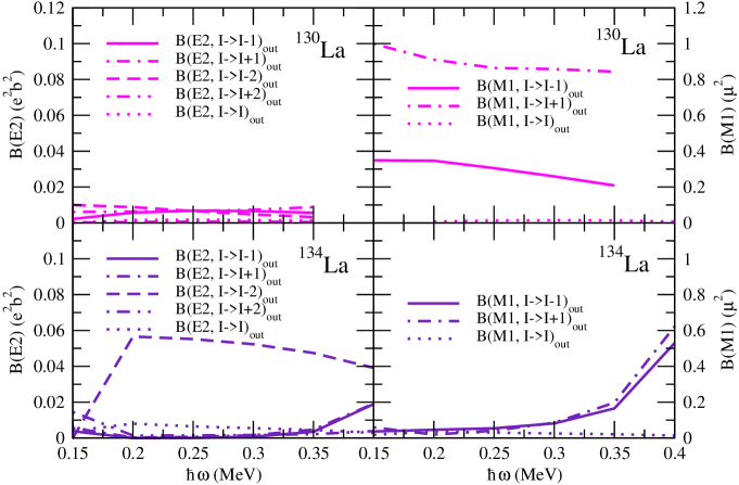
Figure 9: The RPA inter-band transition rates in ¹³⁰La and ¹³⁴La.

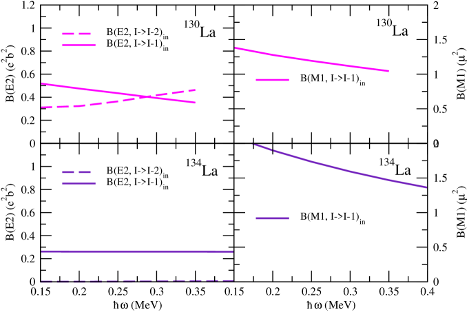
Figure 10: The TAC intra-band transition rates in ¹³⁰La and ¹³⁴La.

The ratios of the different transition probabilities vary substantially over the studied region. The $B(E2,I\rightarrow I\pm 1)$ and $B(M1,I\rightarrow I\pm 1)$ are typically the strongest.

There are experimental data for the inter-band transition rates in ¹³⁴Pr TA07 . Our calculated rates are somewhat larger than the ones seen in experiment. There are also data available for the ratio of $B(M1)_{out}/B(M1)_{in}$ in ¹³⁶Pm HR01 , but unfortunately not in the frequency range where we have RPA results.

IV Shape and orientation oscillation amplitudes

The energies and the transition rates do not give direct information about the character of the RPA phonon. The question is, if it represents predominantly oscillations of the orientation of the quadrupole tensor relative to the angular momentum vector, which we then classify as chiral vibrations, or predominantly oscillations of the deformation parameters, or a combination of both types of oscillation. From the curvature of potential energy surfaces as seen in Fig. 1 and 2 one can only make some qualitative guesses. In the following we determine quantitatively the size of shape and angle oscillations of the RPA phonon.

The RPA describes quantized oscillations of the quadrupole tensor relative to the uniformly rotating quadrupole tensor of the self-consistent TAC solution. As well known, the explicit time dependent state $|t\rangle$ corresponding to TAC+RPA is the small amplitude periodic solution of the time dependent mean field problem (TDHF, cf. e.g. Negele82 ). The TAC solutions are found in the P-coordinate system, which uniformly rotates about the z-axis of the L-system. Within the P-frame, the quadrupole tensor of the TAC solution does not depend on time, and $\langle\hat{Q}_{\pm 1}\rangle$=0 and $\langle\hat{Q}_{2}\rangle$=$\langle\hat{Q}_{-2}\rangle$. The time dependence is generated by the RPA correlations, which are reflected by transition matrix elements of the quadrupole tensor. It is useful to consider the set $\hat{Q}_{{}_{k\pm}}$ of hermitean quadrupole operators defined by

$$\hat{Q}_{{}_{1+}} = \frac{\hat{Q}_{{}_{1}}+\hat{Q}_{{}_{-1}}}{i\sqrt{2}},\quad\hat{Q}_{{}_{1-}}=\frac{\hat{Q}_{{}_{1}}-\hat{Q}_{{}_{-1}}}{\sqrt{2}},$$

$$\hat{Q}_{{}_{2+}} = \frac{\hat{Q}_{{}_{2}}+\hat{Q}_{{}_{-2}}}{\sqrt{2}},\quad\hat{Q}_{{}_{2-}}=\frac{\hat{Q}_{{}_{2}}-\hat{Q}_{{}_{-2}}}{i\sqrt{2}}.$$ (19)

As discussed in the Appendix, their mean values oscillate with the frequency $\Omega$ corresponding to RPA phonon excitation energy $E_{{}_{RPA}}=\hbar\Omega$, and the TDHF state can be normalized such that the amplitudes are equal to the transition matrix elements, i. e.

$$\langle t|\hat{Q}_{{}_{k\pm}}|t\rangle-\langle\hat{Q}_{{}_{k\pm}}\rangle=\langle 1|{\hat{Q}}_{{}_{k\pm}}|0\rangle\cos\Omega t\equiv\Delta Q_{{}_{k\pm}}\cos\Omega t.$$ (20)

The quadrupole oscillations can be decomposed into oscillations of the shape parameters $\varepsilon$ and $\gamma$ ($\beta$ and $\gamma$ vibrations, respectively) and into oscillations of the orientation angles $\vartheta$, $\varphi$, and $\psi$ of the principal axes of quadrupole tensor with respect to the uniformly rotating P-system. That is, we derive a new set of transition amplitudes $\Delta\vartheta$, $\Delta\varphi$, and $\Delta\psi$, representing the chiral vibrational part of the excitation, and $\Delta\varepsilon/\varepsilon$ and $\Delta\gamma$ representing the shape oscillation part. Exploiting the shape selfconsistency conditions (II), $\langle\hat{Q}_{{}_{0}}\rangle=C\,\varepsilon\cos{\gamma}$ and $\langle\hat{Q}_{{}_{2+}}\rangle=-C\,\varepsilon\sin{\gamma}$, where $C=2/3\,\hbar\omega_{{}_{0}}/\kappa_{{}_{0}}$, we derive in the Appendix

$$\frac{\Delta\varepsilon}{\varepsilon} = \frac{\langle\hat{Q}_{{}_{0}}\rangle\Delta Q_{{}_{0}}+\langle\hat{Q}_{{}_{2+}}\rangle\Delta Q_{{}_{2+}}}{\langle\hat{Q}_{{}_{0}}\rangle^{2}+\langle\hat{Q}_{2+}\rangle^{2}},$$ (21)

$$\Delta\gamma = \,\frac{\langle\hat{Q}_{{}_{2+}}\rangle\Delta Q_{{}_{0}}-\langle\hat{Q}_{{}_{0}}\rangle\Delta Q_{{}_{2+}}}{\langle\hat{Q}_{{}_{0}}\rangle^{2}+\langle\hat{Q}_{2+}\rangle^{2}}.$$ (22)

Considering the following small rotations

$$R_{3} = 1-i\Delta\varphi\hat{J}_{3},$$

$$R_{2} = 1-i\Delta\vartheta\hat{J}_{2},$$

$$R_{z} = 1-i\Delta\psi\hat{J}_{z}=1-i\Delta\psi(\cos{\vartheta}\hat{J}_{3}+\sin{\vartheta}\hat{J}_{1}),$$ (23)

where the angular momentum operators are taken in RPA order, and evaluating the expectation values $\langle R_{i}\hat{Q}_{{}_{k}}R_{i}\rangle$ we derive in the Appendix

$$\Delta\varphi = \frac{\Delta Q_{{}_{2-}}}{2\langle\hat{Q}_{{}_{2+}}\rangle}-\Delta\psi\cos{\vartheta},$$ (24)

$$\Delta\vartheta = \frac{\Delta Q_{{}_{1-}}}{\langle\hat{Q}_{{}_{2+}}\rangle-\sqrt{3}\langle\hat{Q}_{{}_{0}}\rangle},$$ (25)

$$\Delta\psi = \frac{\Delta Q_{{}_{1+}}}{\,\sin{\,\vartheta}\,(\langle\hat{Q}_{{}_{2+}}\rangle+\sqrt{3}\langle\hat{Q}_{{}_{0}}\rangle)}.$$ (26)

Similar equations were derived by Shimizu and Matsuzaki SM96 (cf. their Eqs.(4.21)) for the wobbling mode, which correspond to the special case $\vartheta=0$ where $\Delta\psi$ becomes zero (see Appendix).

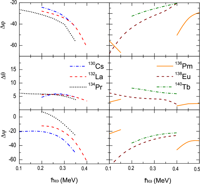
Figure 11: (Color online) The amplitudes of the Euler angles in degrees in the lowest RPA phonons of the N=75 isotone chain. Cs, La and Pr in the left panels and Pm, Eu and Tb in the right panels.

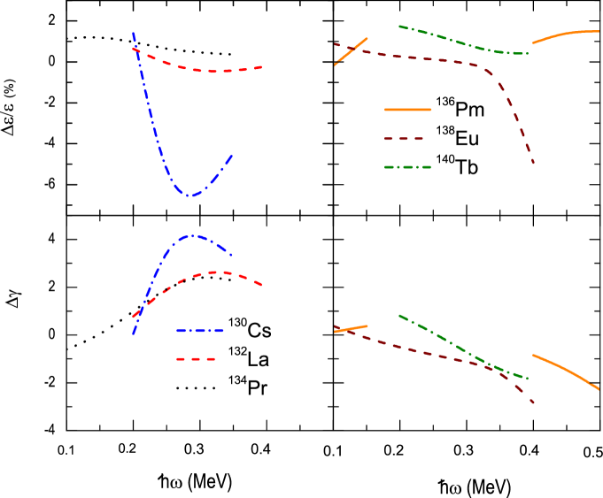
Figure 12: (Color online) The amplitudes of shape parameters in the lowest RPA phonons in the N=75 isotone chain ($\gamma$ in degrees). Cs, La and Pr in the left panels and Pm, Eu and Tb in the right panels.

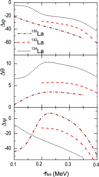
Figure 13: (Color online) The amplitudes of Euler angles in degrees in the lowest RPA phonons in the Z=57 isotones.

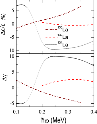
Figure 14: (Color online) The amplitudes of shape parameters in the lowest RPA phonons in the Z=57 isotones ($\gamma$ in degrees).

The results are shown in Fig. 11 and 12. One can clearly see that the lowest phonon is dominated by orientation oscillations, especially in the $\varphi$ direction, which is consistent with the TAC potential energy surface in Fig. 2. The amplitude $\Delta\varphi$ starts at 30-40^∘ and increases toward the point where the RPA energy goes to zero. It diverges at the transition to aplanar chiral rotation. As discussed above, this can happen with increasing or decreasing $\omega$, depending on the nuclide. The amplitudes $\Delta\psi$ behave in the same way, being somewhat smaller than $\Delta\varphi$. The amplitude of the $\vartheta$-oscillations is 5-10^∘. In all cases, the shape oscillations are small in amplitude compared to the orientation oscillations. The amplitudes $\Delta\varepsilon$ are few percent of the equilibrium values and $\Delta\gamma<6^{o}$ for all cases but ¹³⁴La (cf. next paragraph). This is in contrast to Ref. TA06 , which, taking into account the shape degrees of freedom in the framework of the the IBAFF two-particle-core approach, found a strong coupling between the shape and orientation degrees of freedom. In our microscopic approach, the lowest phonon is a rather clean chiral vibration.

Figures 14 and 14 show how the structure of the lowest RPA phonon develops when moving away from the N=75 chain. In the N=73 nuclide ¹³⁰La, the angle oscillations also dominate although $\gamma$ vibration becomes more important at large $\omega$. This is consistent with a reduced stability of the triaxial deformation, which eventually disappears with decreasing N. In ¹³⁴La with N=77 we are approaching the N=82 shell closure, which leads to a reduction in the deformation and increased amplitudes of the shape oscillations in the RPA phonon. The case of ¹³⁴La can no longer be thought of as a chiral vibration even though it has large components of orientation oscillations in the wave function. The large jump in several of the ¹³⁴La curves is due to the level crossing between the first and second RPA solution seen in Fig. 4.

V Conclusions

We have combined the TAC mean field approach with the RPA for a modified Quadrupole-Quadrupole interaction in order to calculate the energy splitting between chiral partner bands, which is given by the excitation energy of the lowest RPA solution. Our TAC+RPA calculations also give the intra- and inter-band transition rates.

By analyzing the RPA amplitudes we found that near Z=57 and N=75 the lowest phonon is a rather pure collective chiral vibration. It represents a slow oscillation of the quadrupole shape relative to the angular momentum vector, which takes wide excursions into the left - and right - handed arrangements of the three principal axes and the angular momentum. The amplitudes of the shape oscillations are found to be much smaller than the ones of the orientation oscillations. The large amplitude nature of the angle oscillations indicate that for a full understanding of the chiral bands one has to take into account effects that go beyond the harmonic RPA approximation in the orientation degrees of freedom. The anharmonicities will change the collective mode in a qualitative way where the energy of the first RPA solution goes to zero and the mean field attains static chirality. This transition is encountered for most of the studied cases. Since our investigation indicates that the shape degrees are well decoupled from the angle ones, it seems promising to try to describe the transition in terms of an effective Hamiltonian depending only on the components of the total angular momentum ADF11 .

Our TAC+RPA calculations give phonon energies in the order of 300 keV or lower, which is comparable with the experimental energy differences between the chiral partner bands. However the trend with increasing angular momentum is not always reproduced. The calculated phonon energy goes to zero where the TAC solution attains static chirality. One would expect TAC+RPA to describe the angular momentum dependence of the energy difference between the partners in a qualitative manner, i.e. reproduce if it is increasing a or decreasing and give zero splitting for static chirality of the TAC solution instead of a finite small splitting seen in experiment. This is the case for ¹³⁴Pr, ¹³⁰Cs, ¹³⁴La, and ¹³⁵Nd MA07 , whose phonon energy decreases with angular momentum, and ¹³⁸Eu, whose phonon energy increases. However, for ^130,132La and ¹³⁶Pm the experimental energy difference between the partner bands is nearly constant 300-400 keV in contrast to the calculations. The reason for the discrepancy is unclear, and it remains to be seen whether a large amplitude description of the chiral mode will be able to account for the experiment. It is also noted that for a number of studied nuclides only few members of the chiral partner band are observed, such that the angular momentum dependence of the phonon energy is not well established. This information would be crucial for a deeper understanding of the onset of chirality.

The calculation of the inter-band transition rates shows that the ratios of the different $\Delta I$ components of the transitions vary relatively fast with N and Z. We could not discern a systematic pattern indicating the onset of chirality.

The quite pure chiral nature of the RPA solution seems to be localized around the N=75 isotones. Moving to more neutron-rich nuclei structure of the first RPA phonon changes to a complex mixture of shape and orientation degrees of freedom, reflecting the approach of the shell closure at N=82. Towards the more neutron deficient nuclides the deformation is increasing but the triaxiality is decreasing, which reduces the collectivity of the lowest RPA solutions that takes on 2qp character.

Appendix A

We consider small-amplitude vibrations about a planar TAC solution in the P-system. The solution of the TDHF equations results in oscillating quadrupole moments

$$\hat{Q}_{{}_{k}}(t)=\langle\hat{Q}_{{}_{k}}\rangle+A\Delta Q_{{}_{k}}\cos{\Omega t},~{}~{}k=0,1\pm,~{}2\pm,$$ (27)

where we refer to the hermitean combination $\hat{Q}_{{}_{k\pm}}$ defined by Eqs. (IV). The periodic TDHF solutions are related to RPA solutions (20) (e. g. see Ref. Negele82 Eqs. (3.37), (3.38)) such that one has

$$E_{{}_{RPA}}=\hbar\Omega,\qquad\Delta Q_{{}_{k}}=\langle 1|\hat{Q}_{{}_{k}}|0\rangle$$ (28)

where $|1\rangle$ corresponds to the lowest RPA excitation. The amplitude of the oscillations is not determined by the TDHF equations. We chose it such that $A=1$.

The oscillations of the quadrupole tensor $\hat{Q}_{{}_{k}}(t)$ can be expressed as oscillations of the shape parameters $\varepsilon$ and $\gamma$ and oscillations of the Euler angles $\varphi$, $\vartheta$ and $\psi$ which determine the orientation of the principal axes of the oscillating quadrupole tensor relative to the P-frame.

We start the derivations with the shape amplitudes $\Delta\varepsilon$ and $\Delta\gamma$. The self consistency conditions (II) state

$$\langle\hat{Q}_{{}_{0}}\rangle\, = \,\,C\,\varepsilon\cos{\gamma},$$

$$\langle\hat{Q}_{{}_{2+}}\rangle = -C\,\varepsilon\sin{\gamma}.$$ (29)

Variation of both sides gives

$$\Delta Q_{{}_{0}}\,\, = \,\,\,C\,(\Delta\varepsilon\cos{\gamma}-\varepsilon\sin{\gamma}\Delta\gamma),$$

$$\Delta Q_{{}_{2+}} = -C\,(\Delta\varepsilon\sin{\gamma}+\varepsilon\cos{\gamma}\Delta\gamma).$$ (30)

Inverting yields the desired relations for the shape amplitudes

$$\frac{\Delta\varepsilon}{\varepsilon} = \frac{\langle\hat{Q}_{{}_{0}}\rangle\Delta Q_{{}_{0}}+\langle\hat{Q}_{{}_{2+}}\rangle\Delta Q_{{}_{2+}}}{\langle\hat{Q}_{{}_{0}}\rangle^{2}+\langle\hat{Q}_{2+}\rangle^{2}},$$ (31)

$$\Delta\gamma = \,\frac{\langle\hat{Q}_{{}_{2+}}\rangle\Delta Q_{{}_{0}}-\langle\hat{Q}_{{}_{0}}\rangle\Delta Q_{{}_{2+}}}{\langle\hat{Q}_{{}_{0}}\rangle^{2}+\langle\hat{Q}_{2+}\rangle^{2}}.$$ (32)

Now we perform rotations $R_{2,3}$ with small angles $\Delta\vartheta$ and $\Delta\varphi$ about the respective axes 2 and 3 of the P-frame and a rotation $R_{z}$ with a small angle $\Delta\psi$ about the $z$-axis of the L-frame (direction of angular momentum). We calculate the change of the quadrupole moments generated by the reoriention, i. e. we take the expectation values with respect to the states $R_{i}|TAC\rangle$. Inverting these relations, will provide us with the angles $\Delta\varphi,\Delta\vartheta,\Delta\psi$ of the principal axes of $\hat{Q}_{k}(t)$ within the P-system. Expanding the corresponding exponential rotational operators up to first order we have

$$R_{{}_{3}} = 1-i\Delta\varphi\hat{J}_{{}_{3}},$$

$$R_{{}_{2}} = 1-i\Delta\vartheta\hat{J}_{{}_{2}},$$

$$R_{{}_{z}} = 1-i\Delta\psi\hat{J}_{{}_{z}}=1-i\Delta\psi(\cos{\vartheta}\hat{J}_{{}_{3}}+\sin{\vartheta}\hat{J}_{{}_{1}}).$$ (33)

In this linear order the rotation operators $R_{i}$ commute and we can arrange them in a new set that performs small rotations about the axes 1,2 and 3:

$$\tilde{R}_{{}_{3}} = 1-i(\Delta\varphi+\Delta\psi\cos{\vartheta})\hat{J}_{{}_{3}},$$

$$R_{{}_{2}} = 1-i\Delta\vartheta\hat{J}_{{}_{2}},$$

$$\tilde{R}_{{}_{1}} = 1-i\Delta\psi\sin{\vartheta}\hat{J}_{{}_{1}}.$$ (34)

We begin with the calculation of the change of the expectation values of the components $\hat{Q}_{{}_{\pm 2}}$ with respect to the rotated state $\tilde{R}_{{}_{3}}|TAC\rangle$. Using Eqs. (A) we obtain

$$\langle\tilde{R}^{\dagger}_{3}\hat{Q}_{{}_{\pm 2}}\tilde{R}_{3}\rangle=\langle\hat{Q}_{{}_{\pm 2}}\rangle+i(\Delta\varphi+\Delta\psi\cos{\vartheta})\langle[\hat{J}_{{}_{3}},\hat{Q}_{{}_{\pm 2}}]\rangle=\langle\hat{Q}_{{}_{\pm 2}}\rangle\pm 2i(\Delta\varphi+\Delta\psi\cos{\vartheta})\langle\hat{Q}_{{}_{\pm 2}}\rangle.$$ (35)

For the hermitian operators $\hat{Q}_{{}_{2\pm}}$ defined by Eqs. (IV) it follows

$$\Delta Q_{{}_{2-}} = 2(\Delta\varphi+\Delta\psi\cos{\vartheta})\langle\hat{Q}_{{}_{2+}}\rangle,$$ (36)

$$\langle\tilde{R}^{\dagger}_{{}_{3}}\hat{Q}_{{}_{2+}}\tilde{R}_{{}_{3}}\rangle = \langle\hat{Q}_{{}_{2+}}\rangle,$$ (37)

where $\langle\hat{Q}_{{}_{2-}}\rangle=0$ was used. Eq.(36) shall be used below to determine $\Delta\varphi$ whereas the last relation (37) expresses the fact that the rotation $\tilde{R}_{{}_{3}}$ does not lead to a shape change $\Delta Q_{{}_{2+}}$. The same is valid for the other components

$$\langle\tilde{R}^{\dagger}_{3}\hat{Q}_{{}_{\pm 1}}\tilde{R}_{3}\rangle = \langle\hat{Q}_{{}_{\pm 1}}\rangle+i\Delta\varphi\langle[\hat{J}_{{}_{3}},\hat{Q}_{{}_{\pm 2}}]\rangle=\langle\hat{Q}_{{}_{\pm 1}}\rangle\pm i(\Delta\varphi+\Delta\psi\cos{\vartheta})\langle\hat{Q}_{{}_{\pm 1}}\rangle=0,$$ (38)

$$\langle\tilde{R}^{\dagger}_{3}\hat{Q}_{{}_{0}}\tilde{R}_{3}\rangle = \langle\hat{Q}_{{}_{0}}\rangle,$$ (39)

where $\langle\hat{Q}_{{}_{1\pm}}\rangle=0$ was used. Now we calculate the components of $\hat{Q}_{{}_{\pm 1}}$ for the rotated state $R_{{}_{2}}|TAC\rangle$. We have

$$\langle R^{\dagger}_{{}_{2}}\hat{Q}_{{}_{\pm 1}}R_{{}_{2}}\rangle=i\Delta\vartheta\langle[\hat{J}_{{}_{2}},\hat{Q}_{{}_{\pm 1}}]\rangle=\pm\frac{\Delta\vartheta}{2}\,(2\langle\hat{Q}_{{}_{2}}\rangle-\sqrt{6}\langle\hat{Q}_{{}_{0}}\rangle)=\Delta Q_{{}_{\pm 1}},$$ (40)

where we used $\hat{J}_{{}_{2}}=-i/2\,(\hat{J}_{{}_{+}}-\hat{J}_{{}_{-}})$ and $\langle\hat{Q}_{{}_{\pm 1}}\rangle=0$ . This gives for the hermitian combination $\hat{Q}_{{}_{1-}}$

$$\Delta Q_{{}_{1-}}=\Delta\vartheta\,(\langle\hat{Q}_{{}_{2+}}\rangle-\sqrt{3}\langle\hat{Q}_{{}_{0}}\rangle),$$ (41)

which yields expression for the amplitude $\Delta\vartheta$, Eq.(25). The other components of the quadrupole tensor do not change because $\langle[\hat{J}_{\pm},\hat{Q}_{\pm 2}]\rangle$ and $\langle[\hat{J}_{\pm},\hat{Q}_{0}]\rangle$ are proportional to $\langle\hat{Q}_{\pm 1}\rangle=0$. Finally we calculate the expectation values of the quadrupole operators $\hat{Q}_{{}_{\pm 1}}$ for $\tilde{R}_{{}_{3}}|TAC\rangle$. Using $\hat{J}_{{}_{1}}=1/2\,(\hat{J}_{{}_{+}}+\hat{J}_{{}_{-}})$ we obtain analogously

$$\langle\tilde{R}^{\dagger}_{1}\hat{Q}_{{}_{\pm 1}}\tilde{R}_{1}\rangle=i\Delta\psi\,\langle[\sin{\vartheta}\hat{J}_{{}_{1}},\hat{Q}_{{}_{\pm 1}}]\rangle=i\frac{\Delta\psi}{2}\,\sin{\vartheta}\,(2\langle\hat{Q}_{{}_{2}}\rangle+\sqrt{6}\langle\hat{Q}_{{}_{0}}\rangle).$$ (42)

Considering the combination $\hat{Q}_{{}_{1+}}$ we get

$$\Delta Q_{{}_{1+}}=\Delta\psi\sin{\vartheta}\,(\langle\hat{Q}_{{}_{2+}}\rangle+\sqrt{3}\langle\hat{Q}_{{}_{0}}\rangle),$$ (43)

which gives the amplitude $\Delta\psi$ by Eq.(26). With help of Eq.(36) the amplitude $\Delta\varphi$ given by Eq.(24) is found.

References

- (1) S. Frauendorf, Rev. Mod. Phys. 73, 463 (2001)
- (2) V.I. Dimitrov, S. Frauendorf and F. Dönau, Phys. Rev. Lett 84, 5732 (2000)
- (3) P. Olbratowski, J. Dobaczewski, J. Dudek and W. Plociennik, Phys. Rev. Lett. 93, 052501 (2004)
- (4) S. Frauendorf and J. Meng, Nucl. Phys. A617, 131 (1997)
- (5) K. Starosta et al., Phys. Rev. C 65, 044328 (2002)
- (6) S. Brant, D. Vretenar and A. Ventura, Phys. Rev. C 69, 017304 (2004)
- (7) D. Tonev et al., Phys. Rev. Lett. 96, 052501 (2006)
- (8) K. Starosta et al., Phys. Rev. Lett 86, 971 (2001)
- (9) A.A. Hecht et al., Phys. Rev. C 63, 051302(R) (2001)
- (10) P. Ring and P. Schuck, The Nuclear Many-Body Problem, (Springer, New York, 1980)
- (11) C.M. Petrache, G.B. Hagemann, I. Hamamoto and K. Starosta, Phys. Rev. Lett. 96, 112502 (2006)
- (12) E. Grodner et al., Phys. Rev. Lett. 97, 172501 (2006)
- (13) S. Mukhopadhyay et al., Phys. Rev. Lett. (2007)
- (14) S. Zhu et al., Phys. Rev. Lett. 91, 132501 (2003)
- (15) S. Frauendorf, Nucl. Phys. A677, 115 (2000)
- (16) M. Barranger and K. Kumar, Nuc. Phys. A110, 490 (1968)
- (17) S. G. Nilsson and I. Ragnarsson, Shapes and Shells in Nuclear Physics (Cambridge University Press, Cambridge, 1995).
- (18) . J. Kvasil and R. Nazmitdinov, Sov. J. Part. Nucl. 17, 265 (1986)
- (19) T. Koike, K. Starosta, C.J. Chiara, D.B. Fossan, and D.R. LaFosse, Phys. Rev. C 67, 044319 (2003)
- (20) D.J. Hartley et al., Phys. Rev. C 64, 031304(R) (2001)
- (21) T. Koike, K. Starosta, C.J. Chiara, D.B. Fossan, and D.R. LaFosse, Phys. Rev. C 63, 061304(R) (2001)
- (22) R.A. Bark et al., Nucl. Phys. A 691, 577 (2001)
- (23) D. Almehed, F. Dönau, and S. Frauendorf, to be published
- (24) D. Tonev et al., Phys. Rev. C 76, 044313 (2007)
- (25) J. W. Negele, Rev. Mod. Phys. 54, 914 (1982)
- (26) Y.R. Shimizu and M. Matsuzaki, Nucl. Phys. A588, 559 (1996)