Multifractal regime transition in a modified minority game model

Abstract

The search for more realistic modeling of financial time series reveals several stylized facts of real markets. In this work we focus on the multifractal properties found in price and index signals. Although the usual Minority Game (MG) models do not exhibit multifractality, we study here one of its variants that does. We show that the nonsynchronous MG models in the nonergodic phase is multifractal and in this sense, together with other stylized facts, constitute a better modeling tool. Using the Structure Function (SF) approach we detected the stationary and the scaling range of the time series generated by the MG model and, from the linear (nonlinear) behavior of the SF we identified the fractal (multifractal) regimes. Finally, using the Wavelet Transform Modulus Maxima (WTMM) technique we obtained its multifractal spectrum width for different dynamical regimes.

I Introduction

In the last years several agents based models for asset returns have been proposed in the literature lux99 ; levylevy . One of the reasons for this interest is that the traditional models derived from the geometrical Brownian motion do not explain adequately many properties of real markets. The Minority Game (MG) and its variants constitute one of the most promising models Challet due to their capability of explaining a wider range of properties found in price and index signals. It is usual to characterize economic time series from their empirical properties called stylized facts rama2001 , which includes multifractal long range correlations. There are several ways to characterize the long-range correlations from the real time series and from its models. Some of these methods are the autocorrelation functions, power spectral densities (either from Fourier or wavelets transforms) and probability distribution functions. In addition, the fractal and the multifractal analysis provide more insights, respectively, on the self-similar and self-affine scaling exponents. Here we use the Hurst exponent obtained from the Structure Function (SF) method sf , and the singularity spectrum obtained from the Wavelet Transform Modulus Maxima (WTMM) method muzy91 ; arneodo95 to determine, respectively, the fractal and the multifractal structure of signals generated by the Minority Game model.

The MG models are an oversimplified version of complex systems. Their peculiarity is that several modifications on the original model are possible in order to make it more realistic and analytically tractable in the stationary state via replica or generating functional methods Challet98 ; Challet99 ; fgeratriz ; Coolen . Such methods have led to a deep understanding of their macroscopic properties. Unfortunately, many interesting phenomena occur in the nonergodic phase where the analytical approach fails. Here we address a version of MG where the synchronicity of time transactions is removed andersen2006 ; matteo2002 ; andrea2003 allowing agents to trade on different time-scales. Remarkably, for different distribution of frequencies, it has been shown that these models essentially preserve many of the statistical features of synchronized MG versions such as phase transition, volatility clustering, fat tail PDFs and so on. However, these features now depend on the distribution of the trading frequency. In the present work we will focus on the case where the amount of information processed by agents is the same.

This investigation is part of our continuing quest to find models that comply with all known stylized facts in financial time evolution fff2003 . Thus it is important to explore the property of multiscaling in the artificially generated data. Many empirical studies have indicated the presence of multifractal behavior in real data as a stylized fact. Surprisingly, MG models incorporate this effect through a more realistic trading rules of agents.

The paper is organized as follows. In Section 2 we describe the model, and then we discuss in Section 3 the statistical properties of the return time series. In Section 4 we explain the multifractal concept and the method used to detect it. The results of the multifractal analysis are discussed in the Section 5. Finally, in the last section we present our conclusions.

II Minority Game with different time-scales

The simplest version of the Minority Game Challet97 consists on a set of $N_{s}$ adaptive agents, also called speculators. They are endowed with $S$ strategies that map public information $\mu\in[{0,\dots,P-1}]$ to the decision of buying or selling assets, $a^{\mu}_{i,s}(t)=\pm 1$, $i=1\ldots N_{s}$, $s=1\ldots S$. Each strategy is generated at the beginning of the game and is kept frozen along the dynamics. Besides, the strategies have a payoff function, $U_{i,s}(t)$, that describes their performance all the time according to the following payoff function:

$$U_{i,s}(t+1)=U_{i,s}(t)-a_{i,s}^{\mu}(t)A(t),$$ (1)

where $A(t)=\sum_{i}a^{\mu}_{i,s^{*}}(t)$ is the excess demand. This rule is applied to all strategies independently of their previous scores. The public information is a non negative integer number drawn at random each round uniformly from in the interval $[0,P)$. The decisions are made according to $a^{\mu}_{i,s^{*}}(t)$, where $s^{*}$ is the label for the best ranked strategy $(s^{*}=max_{s}~{}U_{i,s})$. In case of a tie, the decision is made based on coin tossing.

An improved model is the grand canonical minority game which consists of two distinct groups, namely, producers and speculators. The producers have one strategy, their decisions are a function of $\mu$ only, and hence they are always doing transactions in the market. The speculators now have an extra strategy, $s=0$, that allows them not to trade when their strategies are not profitable enough. We compute the strategies’ performance with the following payoff function

$$U_{i,s}(t+1)=U_{i,s}(t)-a_{i,s}^{\mu}(t)A(t)+\epsilon\delta_{0,s}$$ (2)

where $\epsilon$ is a small real number, which can be positive (interest rate) or negative (agent’s risk aversion measure). Thanks to the null strategy, the number of traders fluctuate along the time evolution.

Agents in the standard MG models trade on the same time-scales and different events also occur with the same frequency. We can improve this simplified assumption by introducing $g$ groups of $N_{s}$ speculators, each one with different time scale $ts_{j}$, where one group $g_{j}$ play a singular minority game or grand canonical minority game for $j=1\ldots g$. All agents, independently of the group, have access to the same information $\mu$ and their payoff function are updated virtually all the time. We will implement the grand canonical version, with only one producer’s group with $N_{p}$ members taking action in the smallest timescale. Those timescales are chosen to be daily, weekly and monthly to resemble the real market. The order parameters take into account the total number of agents and it is written as $\alpha=\frac{P}{gN}$.

Other authors andersen2006 ; matteo2002 ; andrea2003 have studied similar models. The basic picture of the behavior of the MG, even considering different distribution of trading time-scales, remains analogous to the synchronized trading frequency model. The control parameter $\alpha$ exhibits some dependence with the distribution frequency parameter. When the time-scale difference $|ts_{i}-ts_{j}|$ increases, for $i\neq j$, the groups become independent and behave as a monochromatic MG. Curiously, the market has the largest fluctuations for small time-scale difference, i.e., when the groups process data that are very close in time.

III Statistical analysis

The minority game models and their variants were extensively explored in several studies. Their capability to generate universal statistical properties qualitatively similar to the financial market have been the main reason for this interest. From the statistical point of view, the known fact is that the probability distribution of returns in the minority game time series is Gaussian except around a critical point. In the subcritical region it is possible to find certain realizations with fat tails but not necessarily following a power law decay. When one allows interaction between groups composed by the players trading in different time scales, the statistical properties are qualitatively preserved.

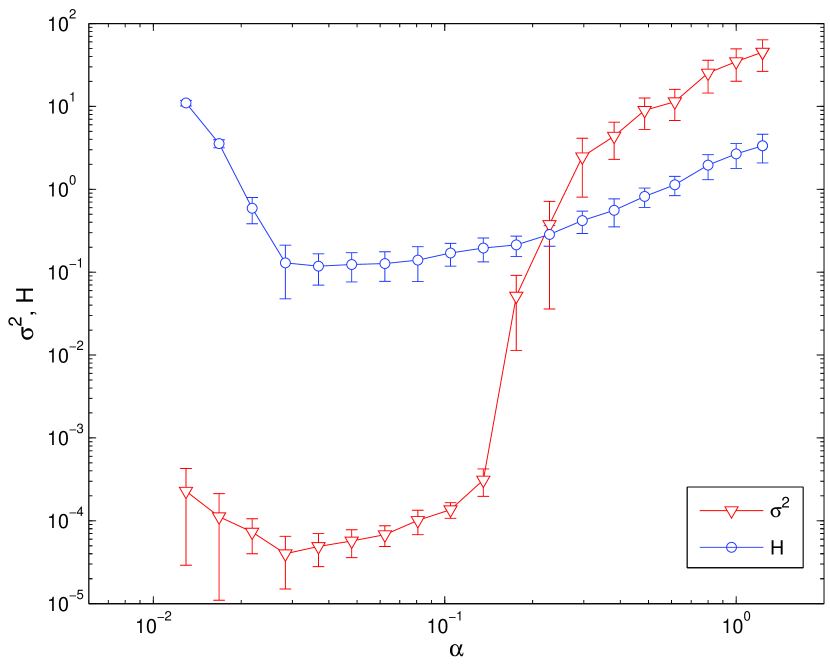
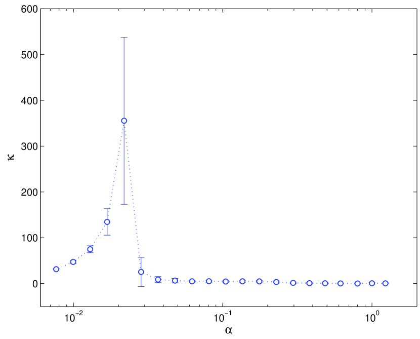
Figure 1: Top: phase diagram for $\sigma$ and H function. Bottom: Kurtosis. The critical value of $\alpha$ occurs for the minimum of the $\sigma$ curve, around $\alpha_{c}=0.2$. The error bars were obtained from 40 realizations of different initial conditions.

Fig. 1(a) presents the variance $\sigma^{2}$ and the predictability $H$ (as a function of $\alpha$) of the return $A(t)$ defined as:

$$H=\frac{1}{P}\sum_{\mu=0}^{P-1}\langle A|\mu\rangle^{2}$$ (3)

where $\langle\ldots\rangle$ is the temporal average. From this plot we can see the phase transition. The critical $\alpha_{c}$ separates the ergodic phase from the nonergodic phase. For $\alpha>\alpha_{c}$ the time series generated by this model has a normal distribution. Fig. 1(a) shows the plots of $\sigma^{2}$ (upper plot) and $H$ (lower plot) against $\alpha$. Qualitatively these these diagrams agree with the synchronous MG model and also they help to locate the value of $\alpha_{c}$. Using the criterion that $\alpha_{c}$ is the minimum of $\sigma$ we find that this value is near 0.2. In Fig. 1(b) we exhibit the kurtosis, denoted by $\kappa$ also as a function of $\alpha$. Firstly, in the low $\alpha$ region, many realizations have high kurtosis and large error bars around $\alpha=0.02$, caused by eventual coordination among agents. It can be shown that for small values of $\alpha$ the time series is leptokurtic.

The next measure we looked at were the probability density functions (PDF) of the fluctuations at different scales. These are simply histograms of the height differences

$$\Delta Y_{\tau}=Y(t+\tau)-Y(t),$$ (4)

where $Y(t)=\sum_{{t^{\prime}}=0}^{t}A(t^{\prime})$ and $\tau$ is the scale. We will also refer to $\tau$ as the scale of analysis.

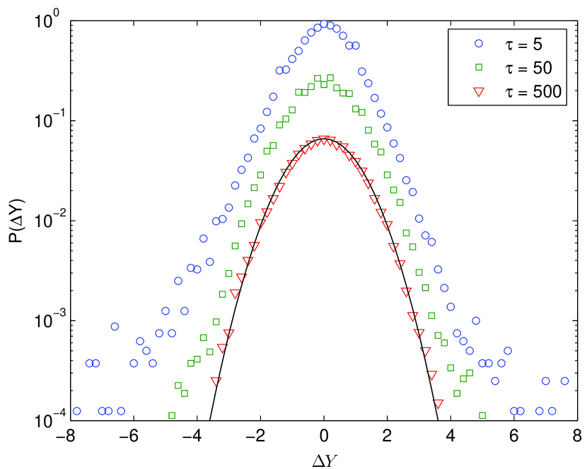
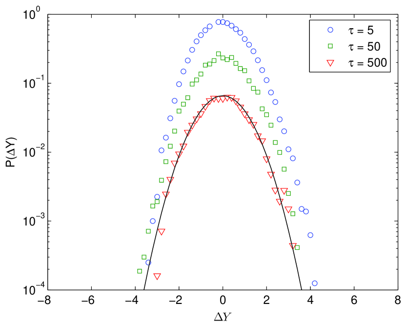
Figure 2: Probability distribution functions for two values of $\alpha$. Top: for $\alpha=0.05$ the PDFs for small scales are fat tailed. Bottom: for $\alpha=0.84$ the PDFs for all scales are gaussians. Shown as reference, the continuous line, the upside down parabola in both panels are gaussians PDFs with zero mean and unit standard deviation.

In the Fig. 2 it is shown the PDFs for two values of $\alpha$, for different dynamical regimes. In the bottom panel, for $\alpha=0.84$, the two groups play independently from each other, and the PDFs for all scales are gaussians. In the top panel, for $\alpha=0.05$, the two groups play interactively and the PDFs are fat tailed for small scales. This is a sign of intermittency frequently found to be related to multifractal processes frisch95 .

IV Structure function analysis

It is usual to characterize the MG dynamics only from the statistical analysis point of view as was done in the section III. In the following we introduce the Structure Function (SF) analysis as a preliminary study to the multifractal scaling.

SF have been largely used in the study of turbulence frisch95 and are defined in the following way sf :

$$S_{q}(\tau)\equiv\langle|Y(t+\tau)-Y(t)|^{q}\rangle\propto\tau^{qh(q)},$$ (5)

where $\langle~{}\rangle$ denotes the ensemble average. The SF can be regarded as a generalization of the correlation functions (when $q=2$). A signal that is scale invariant and self-similar is called fractal when $h(q)$ is the same for all $q$, otherwise it is multifractal paladin87 . Another feature of the SF method is its capability to identify nonstationarity in the data: for stationary time series the exponent of the SF is zero, due to the translational invariance of all statistics.

The time series analysis of the standard MG was done in fff2003 using the unit root test and it was found that the MG time series returns are stationary. To extend the analysis to the present model, we first verified that the SF of the returns, $A(t)$, for $q$ in the range $[1,6.5]$ were all flat for time series $100,000$ points long, indicating that the signal is stationary. Although the time series for the returns was found stationary in a broad range, ones still needs to determine the scaling regime for the cumulative sum of the returns, $Y(t)$, since its scaling range does not necessarily follows the stationary range.

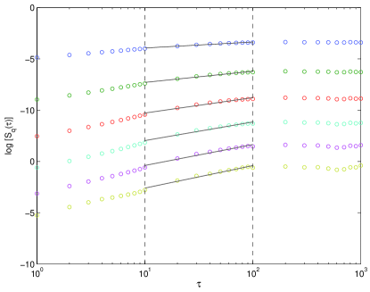
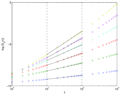
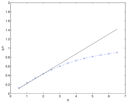
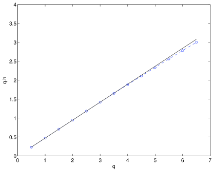
Figure 3: Top row: structure functions, $S_{q}(\tau)$, for the signal $Y(t)$, in arbitrary vertical scales, with dashed vertical lines indicating the scaling range. From top to bottom, the curves are for $q=1.0,2.0,...6.0$. Bottom row: the scaling of the structure functions as given by Eq. 5: when $h(q)$ is not constant with $q$, the signal is said multifractal (bottom, left panel), otherwise the signal is fractal (bottom, right panel). In these panels, the continous line slope gives $h(q=2)$, the Hurst exponent. The left column is for $\alpha=0.05$ and, the right one, for $\alpha=0.84$.

This difference between the stationary range and the scaling range is seen in the SF of $Y(t)$ for $\alpha=0.05$, panel a) in the Fig. 3. These curves are clearly flat for $\tau>1000$. This does not occur for $\alpha=0.84$, panel b) in the same figure, that seems to have a scaling range broader than for $\alpha=0.05$. The superior limit for the scaling range is in general different for different values of $\alpha$: we chose the value $\tau=100$, indicated by the dashed vertical line in the panels a) and b), as the superior limit that is met for all values of $\alpha$. While the scaling range limit on the right is believed to be due information limits, on the left the scaling range is limited by a different reason. Close to the interaction scale, $\tau=5$ in the present simulations, that is below the scaling range, the system does not have yet statistical similarity. We will return to this left limit in the next section. In short, panels a) and b) of Fig. 3 show clearly that the statistical $q$ order moments follow scaling laws. Now we need to identify what is the dependence of these scaling exponents with $q$.

The bottom line of Fig. 3 shows the scaling of the SF as given by Eq. 5, $qh(q)$, against $q$. For $\alpha=0.05$, panel c), the dependence is nonlinear with $q$, indicating that the signal is multifractal, but for $\alpha=0.84$, panel d), the dependence is linear, indicating that the signal is fractal. For reference, in the bottom panels, the slope of the continuous line gives $H$, the Hurst exponent. Although $q$ may be in principle any real number, negative moments are difficult to evaluate due to divergence problems and will be treated using the WTMM method in the next section.

V Multifractal analysis

A given signal can be considered as self-similar with scaling exponent $h$ if its statistical properties are invariant under simultaneous transformation of time $t$ and amplitude $Y(t)$ feder88 ,

$$t\rightarrow bt\equiv t^{\prime};\hskip 56.9055ptY\rightarrow b^{h}Y\equiv Y^{\prime};$$ (6)

where $b$ is an arbitrary positive constant and $h$ is a scaling exponent given by the equation (5). A usual method to compute $h$ is based on the SF approach, as shown in the section IV.

To obtain the full multifractal spectrum we make use of the Wavelet Transform Modulus Maxima (WTMM) method. The wavelet family used in this paper is the $n^{th}$-derivative of the Gaussian density function(DOG$n$), whose wavelet transform has $n$ vanishing moments and removes polynomial trends of order $n-1$ from the signal. Because the scaling properties of the signal are preserved by the wavelet transform, it is possible to obtain its multifractal spectrum using this method. The number of vanishing moments for the wavelet basis, $n$, is chosen to match the order up to ($n-1$) of the polynomial trends in the signal.

The wavelet transform of a signal $Y(t)$ is defined as:

$$T_{\psi}(\tau,b_{0})=\frac{1}{\tau}\sum^{N}_{t=1}Y(t)\psi^{*}\Big{(}\frac{t-b_{0}}{\tau}\Big{)},$$ (7)

where $\tau>0$ is the scale being analyzed, $\psi$ is the mother wavelet DOG$n$ and $N$ is the number of points in $j$ direction. In this paper we used $n=4$ for all analyses.

The statistical scaling properties of the singular measures found in time series can be characterized by the singularity spectrum, $D(h)$, of the Hölder exponents, $h$. A possible approach to obtain the singularity spectrum directly from the time series is the WTMM method muzy91 ; arneodo95 . The singularity spectrum, $D(h)$, and the Hölder exponents, $h$, are obtained from the time series by the following equations:

$$h(q) = \lim_{\tau\rightarrow 0}\frac{1}{\ln\tau}\sum_{\{b_{i}(\tau)\}}\hat{T}_{\psi}[q;\tau,b_{i}(\tau)]\ln\left|T_{\psi}[\tau,b_{i}(\tau)]\right|$$ (8)

$$\equiv \lim_{\tau\rightarrow 0}\frac{1}{\ln\tau}Z(q;\tau)$$

$$D(h) = \lim_{\tau\rightarrow 0}\frac{1}{\ln\tau}\sum_{\{b_{i}(\tau)\}}\hat{T}_{\psi}[q;\tau,b_{i}(\tau)]\ln\big{|}\hat{T}_{\psi}[q;\tau,b_{i}(\tau)]\big{|}$$ (9)

$$\equiv \lim_{\tau\rightarrow 0}\frac{1}{\ln\tau}Z^{*}(q;\tau)$$

where

$$\hat{T}_{\psi}[q;\tau,b_{i}(\tau)]=\frac{\left|T_{\psi}[\tau,b_{i}(\tau)]\right|^{q}}{\sum_{\{b_{i}(\tau)\}}\left|T_{\psi}[\tau,b_{i}(\tau)]\right|^{q}}$$ (10)

and the sum is over the set of the WT modulus maxima footnote at scale $\tau$, ${\{b_{i}(\tau)\}}$. The singularity spectrum, $D(h)$, and the Hölder exponents, $h$, are obtained from scaling range of the plots of Equations (8) and (9), indicated by the dashed vertical lines in the Fig. 4. Each curve on the figure corresponds to different values of $q$. For large and small scales, the scaling regime is broken: to the right, it saturates when the system reaches some physical limits and, to the left, the system is in the range where the agents interacts. The multifractal spectrum is in the Fig. 5.

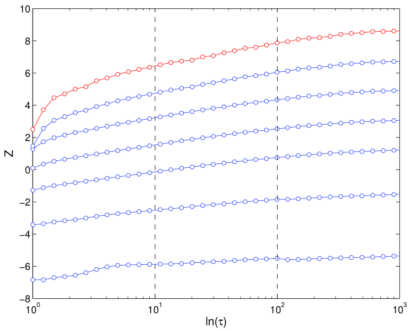
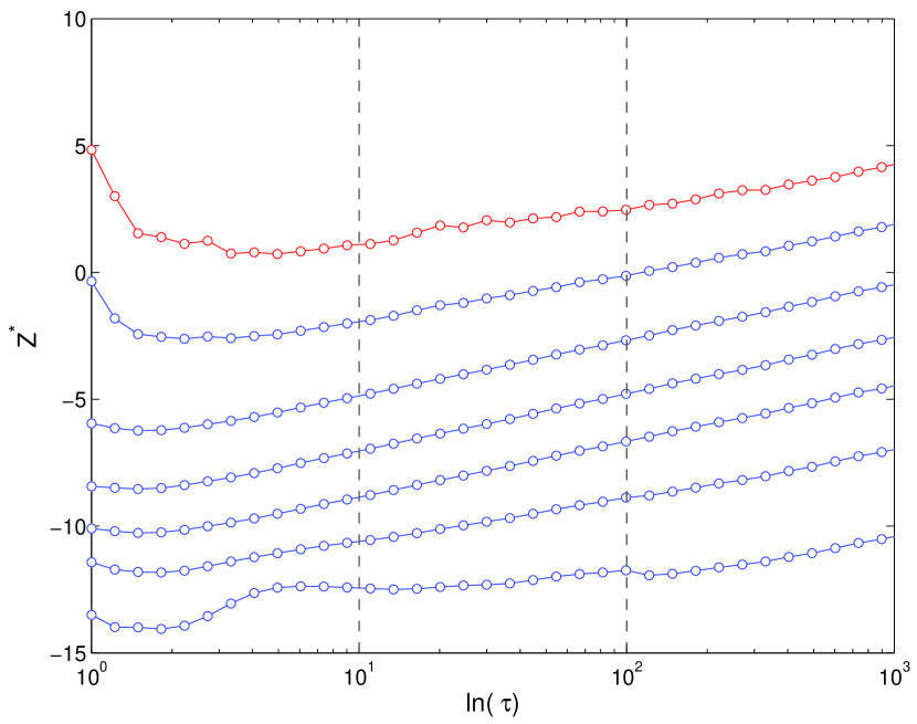
Figure 4: The functions $Z$ (top panel) and $Z^{*}$ (bottom panel), as given by Eq. 8 and Eq. 9, for $\alpha=0.05$. The dashed vertical lines show the scaling region used to obtain $h(q)$. Each curve corresponds to different values of $q$.

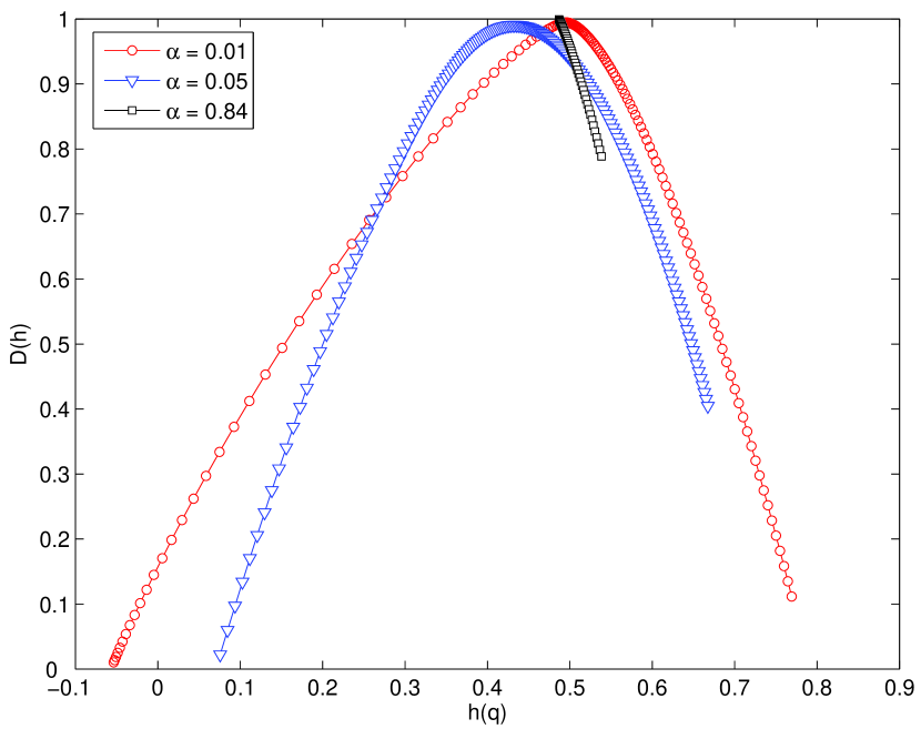
Figure 5: Multifractal spectra for three values of $\alpha=0.01,0.05$ and $0.84$. These values of $\alpha$ are, respectively, for a multifractal regime in the non-ergodic phase, a multifractal regime in the transition region and a fractal regime in the ergodic phase.

One way to interpret the multifractal spectrum in a physical sense is by comparison with the Hurst exponent for known signals, for instance, the fractional Brownian motion feder88 ; mandelbrot68 . The fractional Brownian motion can be classified according to the probabilities of its fluctuations. The usual Brownian motion, obtained from a Gaussian white noise, has the same probability of having positive or negative fluctuations and $H=0.5$. A fractional Brownian motion with $H<0.5$ is more likely to have the next fluctuation with opposite sign with respect to last one – it is said to be antipersistent. Conversely, a fractional Brownian motion with $H>0.5$ is more likely to have the next fluctuation with the same sign as the last one – it is said to be persistent. Antipersistent signals have more local fluctuations and seem more irregular in small scales. Their variance diverges slower with time than the variance of persistent signals. Such signals fluctuate on larger scales and look smoother. This discussion is done in superficie2006 and a similar, but more detailed interpretation, is given in whatcolor2000 .

Now we will analyse for the fractal/multifractal properties of the models’ dynamics as a function of the control parameter $\alpha$. In the ergodic regime, $\alpha=0.84$, Fig. 5 shows that the multifractal spectrum is narrow, almost collapsed to a single point. As already expected, this region is clearly fractal, since the time series for the returns is Gaussian. Just before the transition, in the subcritical regime, the spectrum is wide, a sign of multifractality.

The multifractal spectrum may be represented by its extrema points, i.e., its minima on the left, $h_{l}$, and on the right, $h_{r}$, as well as the maximum (top), $h_{0}$. It is worth to note that a wide spectrum (difference between $h_{r}$ and $h_{l}$) is a clear evidence for the multifractal character of the time series.

We studied the behavior of the extrema points as a function of $\alpha$ to characterize the transition from the fractal to the multifractal regime, as shown in the Fig. 6. This figure shows that the spectrum width increases as $\alpha$ decreases, going from a fractal to multifractal regime. This transition is smooth and exhibits large fluctuation of $h_{l}$ in the nonergodic phase. The point $h_{l}$, which shows the scaling of the fluctuation of the signal, is sensitive to the realization of the trajectory. On the other hand, $h_{r}$ captures the scaling of the small fluctuation. The point $h_{0}$ fluctuates slightly close to 0.5 which is the value observed for random walks.

In the nonergodic, sub-critical phase, the system is said to represent an efficient market, where no arbitrage is possible: this is coherent with the multifractal nature of the time series since this dynamics is richer than the fractal one, that is typical on the ergodic phase.

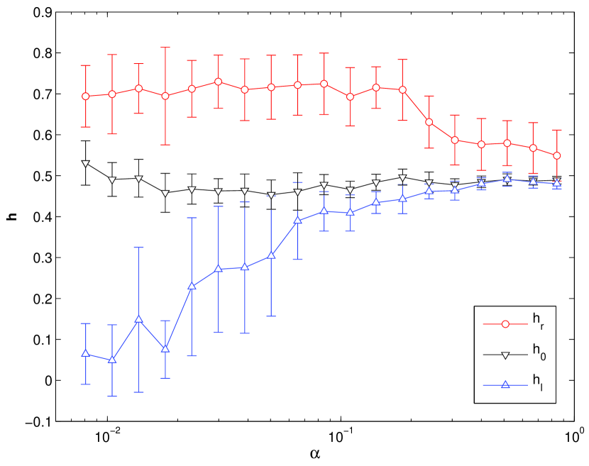
Figure 6: Extrema points of the Multifractal spectra, $h_{l}$, $h_{0}$ and $h_{r}$, for $\alpha$ values from $0.008$ to $0.84$. The signature of multifractality is in the fact that the difference $h_{r}-h_{l}$ increases as $\alpha$ decreases below $\alpha_{c}=0.2$. In the region $\alpha>\alpha_{c}$, where data are Gaussian, this difference should be vanishingly small for time series with infinite number of points. The error bars were obtained from 20 realizations of different initial conditions.

VI Conclusion

We showed that the MG model presents a very rich dynamics with anomalous fluctuations that arise due to strong correlation similar to the one observed in systems driven out of equilibrium. One of the more difficult stylized fact to obtain from models for financial systems are the long range correlations that generate the fractal and multifractal properties present in real time series. The synchronous MG model does not present multifractality. However, only one ingredient added to the model generates multifractal region on the space control parameter $\alpha$. This ingredient was the broken of synchronicity. As the statistical properties of the MG are preserved, the observed multifractal regime belongs to the nonergodic phase, where the market is informationally efficient.

Although the MG time series are not stationary, their increments are. Using the SF approach we detected the stationary range of the increments and the scaling range from the time series. From the linear (non-linear) behavior of the SF we identified the fractal (multifractal) regimes as functions of $\alpha$. To look at the negative values of the moments $q$ we used the WTMM and obtained the full multifractal spectrum against $\alpha$.

- (1) T. Lux and M. Marchesi, Nature 397, 498–500 (1999)
- (2) M.Levy, H.Levy and S.Solomon, Economics Letters 45, 103–111 (1994)
- (3) D.Challet, M.Marsili and Y.-C.Zhang, Minority Games – interacting agents in financial markets (Oxford University Press, New York, 2005)
- (4) Rama Count, Quantitative Finance 1, 223–236 (2001)
- (5) C.X.Yu, M.Gilmore, W.A.Peebles and T.L.Rhodes, Physics of Plasmas 10 (7), 2772–2779 (2003)
- (6) J.Muzy, E.Bacry and A.Arneodo, Phys. Rev. Lett. 67(25), 3515–3518 (1991)
- (7) A.Arneodo, E.Bacry and J.Muzy, Physica A 213, 232–275 (1995)
- (8) D.Challet, and Y.-C.Zhang, Physica A 256, 514–532 (1998)
- (9) D.Challet, and M.Marsili, Physical Review E 60, R6271–R6274 (1999)
- (10) C.De Dominicis, Physical Review B 18, 4913 (1978)
- (11) A.C.C.Coolen, J.A.F.Heimel and D.Sherrington, Physical Review E 65, 016126 (2001)
- (12) J.Wohlmuth and J.V.Andersen, Physica A 363, 459–468 (2006)
- (13) M.Marsili and M.Piai, Physica A 310, 234–244 (2002)
- (14) A.De Martino, Eur. Phys. J. B 35, 143– 152 (2003)
- (15) F.F.Ferreira, G.Francisco, B.S.Machado and P.Muruganandam, Physica A 321, 619–632 (2003)
- (16) D.Challet and Y.-C.Zhang, Physica A 246, 407–418 (1997)
- (17) U.Frisch Turbulence (Cambridge University Press, Cambridge, 1995)
- (18) G.Paladin and A.Vulpiani, Phys. Rep. 156(4), 147–225 (1987)
- (19) While we used routines for the wavelet transforms from C. Torrence and G. Compo, available at URL: http://paos.colorado.edu/research/wavelets/, the WTMM method itself was our own implementation.
- (20) J.Feder, Fractals (Plenum Press, New York, 1988)
- (21) B.Mandelbrot and J.van Ness SIAM Review 10, 422–437 (1968)
- (22) K.Bube, C. Rodrigues Neto, R.Donner, U.Schwarz and Ulrike Feudel, Journal of Physics D: Applied Physics 39, 1405–1412 (2006)
- (23) J.B.Cromwell and W.CLabys and E.Kouassi, Empirical Economics 25, 563–580 (2000)