The combinatorics of associated Hermite polynomials

Abstract.

We develop a combinatorial model of the associated Hermite polynomials and their moments, and prove their orthogonality with a sign-reversing involution. We find combinatorial interpretations of the moments as complete matchings, connected complete matchings, oscillating tableaux, and rooted maps and show weight-preserving bijections between these objects. Several identities, linearization formulas, the moment generating function, and a second combinatorial model are also derived.

The associated Hermite polynomials are a sequence of orthogonal polynomials considered by Askey and Wimp in [AW84], who analytically derived a number of results about these polynomials. They are also treated in [Ism05, Section 5.6]. In section 1 we provide a combinatorial interpretation of these polynomials, their moments, and describe an involution that proves the orthogonality and $L^{2}$ norms of the polynomials with respect to those moments. Then in section 2 we shall describe several linearization formulas involving associated Hermite polynomials. We finish with weight-preserving bijections between a number of classes of combinatorial objects whose generating functions all yield the moments of the associated Hermites, and a second combinatorial model for the polynomials.

We will assume that the reader is familiar with Viennot’s general combinatorial theory of orthogonal polynomials [Vie83, Vie85] and with the combinatorics of Hermite polynomials; see [AGV82, dSCV85, LY89] and also [Vie83, §II.6]. In this paper we use $[n]$ to mean the set of integers $1$ to $n$, inclusive, and write $[n]\sqcup[m]$ for the disjoint union of two such sets.

1. Definition and orthogonality

The associated Hermite polynomials may be defined by shifting the recurrence relation for the usual Hermite polynomials, which is

$$H_{n+1}(x)=xH_{n}(x)-nH_{n-1}(x),$$

to

(1.1) $$H_{n+1}(x;c)=xH_{n}(x;c)-(n-1+c)H_{n-1}(x;c),$$

with $H_{0}(x)=H_{0}(x;c)=1$ and polynomials with negative indices equal to zero. Askey and Wimp use a different normalization than we do; one obtains our normalization from plugging $x/\sqrt{2}$ and $c-1$ into their associated Hermites and dividing by $\left(\sqrt{2}\right)^{n}$.

The usual Hermite polynomial $H_{n+1}(x)$ is the generating function for incomplete matchings of $[n+1]$, in which fixed points have weight $x$ and edges have weight $-1$; that combinatorial interpretation can be derived from the recurrence relation as follows: the vertex $n+1$ may be fixed with weight $x$, times the weight of all matchings on $[n]$; or we may connect vertex $n+1$ to any of the $n$ vertices to its left, give the edge weight $-1$ and multiply by all matchings on the $n-1$ remaining vertices.

For the associated Hermites, we’ll build the matchings recursively as described above and think of the parameter $c$ as meaning that one special choice for the edge from $n+1$ will have weight $-c$. Two natural choices are to make the special choice be the leftmost available vertex, or the rightmost available vertex. Choosing the rightmost available vertex happens to make the orthogonality involution easy to prove, and yields the following result:

Theorem 1.1.

The $n$th associated Hermite polynomial is the sum over weighted incomplete matchings $M$ of $[n]$:

(1.2) $$H_{n}(x;c)=\sum wt(M),$$

in which fixed points have weight $x$, edges that nest no fixed points or edges and have no left crossings have weight $-c$, and all other edges have weight $-1$.

Proof.

We build the matching from right to left, and if at some point we add an edge and do not choose the rightmost available vertex, then that edge will nest a vertex, and when we come to that vertex, we will either leave it fixed (resulting in a fixed point underneath that edge), connect to another vertex underneath the edge (resulting in an edge nested by the original edge), or connect to a vertex to the left of the edge, resulting in a left crossing for the original edge. Any of these possibilities indicate that the rightmost vertex was not chosen, so edges for which none of those happen must have weight $-c$. ∎

An example of such a weighted matching is shown in Figure 1.1.

Figure 1.1. A matching on $7$ points using the rightmost-choice weighting. This weighting is used throughout this paper.

With nothing more than this model, we can easily explain an “unexpected” limit that Askey and Wimp derive [AW84, eq. (5.9)]. (In their paper, there is a small typo: it should be $H_{n}(x\sqrt{2c};c)$.) Using our normalizations, the limit is

(1.3) $$\lim_{c\to\infty}c^{-n/2}H_{n}(x\sqrt{c};c)=U_{n}(x),$$

where $\{U_{n}(x)\}_{n\geq 0}$ are the Chebyshev polynomials of the second kind, also known as Fibonacci polynomials [Vie83, §II.1], [dSCV85]. $U_{n}(x)$ may be thought of as the generating function for incomplete matchings on $n$ vertices in which edges always connect adjacent vertices and have weight $-1$, and fixed points have weight $x$.

Using that combinatorial interpretation for $U_{n}(x)$ and the above interpretation for $H_{n}(x;c)$, there is nothing unexpected about this limit: take $H_{n}(x\sqrt{c};c)$ and give each vertex, whether fixed or incident to an edge, weight $1/\sqrt{c}$, so that $c^{-n/2}H_{n}(x\sqrt{c};c)$ is the generating function for incomplete matchings with fixed points weighted $x$, and all edges weighted $-1/c$ except those which nest no fixed points or edges, and have no left crossings—such edges have weight $-1$. As $c$ goes to infinity, we effectively restrict the generating function to matchings in which no edge has weight $-1/c$; i.e., every edge nests no fixed points or edges, and has no left crossings, so every edge must connect adjacent vertices.

We want a linear functional $\mathcal{L}_{c}$ with respect to which the associated Hermite polynomials are orthogonal. This linear functional is determined by its moments $\mathcal{L}_{c}(x^{n})$, which according to Viennot’s general combinatorial theory of orthogonal polynomials, can be expressed as a sum over weighted Dyck paths in which a northeast edge has weight $1$ and a southeast edge leaving from height $j$ has weight $j-1+c$. There are no Dyck paths of odd length, so the odd moments are zero. The first few nonzero moments are

$$\mu_{0} =1, \mu_{4} =2c^{2}+c,$$

$$\mu_{2} =c, \mu_{6} =5c^{3}+7c^{2}+3c.$$

Using the bijection from weighted Dyck paths to complete matchings from [Vie83, §II.6], we have two combinatorial interpretations for the moments:

Theorem 1.2.

The $n$th moment $\mu_{n}(c)$ of the associated Hermite polynomials is the generating function for complete matchings of $[n]$ weighted by either: (1) edges which are not nested by any other edge have weight $c$, and all other edges have weight $1$; or (2) edges with no right crossings have weight $c$ and all other edges have weight $1$.

The two weightings correspond to giving weight $c$ to the leftmost and rightmost choice, respectively, in the matchings. These interpretations also explain why the odd moments are zero, since there are no complete matchings on an odd number of vertices. For the proof of orthogonality, we shall use the rightmost weighting; later we shall use the leftmost weighting. Figures 1.2 and 1.3 show a matching using the two weightings.

Figure 1.2. A complete matching on $6$ points under the leftmost-choice weighting for the moments, in which nonnested edges have weight $c$ and others have weight $1$.

Figure 1.3. The same complete matching under the rightmost-choice weighting, in which edges with no right crossing have weight $c$ and others have weight $1$. This is used in the orthogonality proof.

1.1. Proof of orthogonality

We wish to prove the following theorem in a combinatorial manner:

Theorem 1.3.

The associated Hermite polynomials $H_{n}(x;c)$ are orthogonal with respect to the linear functional $\mathcal{L}_{c}$ with the above moments. They satisfy

(1.4) $$\mathcal{L}_{c}(H_{n}(x;c)H_{m}(x;c))=\begin{cases}0&n\neq m,\\ (c)_{n}&n=m.\end{cases}$$

Here $(a)_{n}$ denotes the rising factorial $a(a+1)\cdots(a+n-1)$.

Proof.

The proof proceeds very similarly to the proof of orthogonality for usual Hermite polynomials. The product $H_{n}(x;c)H_{m}(x;c)$ is the generating function for pairs of matchings with, say, black edges, using the rightmost weighting. Applying $\mathcal{L}_{c}$ has the effect of putting a complete matching with the rightmost weighting with, say, green edges on the fixed points. We will use the phrase paired matching to refer to such an object, with black homogeneous edges and arbitrary green edges, weighted as above. This is not standard terminology; it is only for our convenience.

Using Theorems 1.1 and 1.2, the left side of (1.4) is the generating function for paired matchings, where black edges have weight $-c$ if they nest no edges, have no green crossings and no left black crossing; otherwise black edges have weight $-1$. Green edges have weight $c$ if they have no right green crossing and weight $1$ otherwise. See Figure 1.4 for an example of such an object for $n=5$ and $m=3$.

Figure 1.4. A paired matching for $n=5$ and $m=3$.

We need an involution that shows the generating function for paired matchings equals zero when $n\neq m$, and equals $(c)_{n}$ otherwise. Assume that $n\geq m$ and put $[n]$ to the left of $[m]$. The involution is the very similar to that used in the combinatorial proof of orthogonality for usual Hermite polynomials:

Find the leftmost homogeneous edge that nests no other edges and change its color.

For example, in Figure 1.4, one would change the color of the leftmost green edge that connects vertices $2$ and $4$ to black. This operation is evidently an involution and will certainly change the sign; we need to verify that the weight of no other edge is affected by this change, and that if we change the color of an edge weighted $\pm c$ or $\pm 1$, the new edge has weight of $\mp c$ or $\mp 1$, respectively.

We begin with the following observation: the leftmost homogeneous edge in $[n]$ that nests no edges can have no left crossing. We must check the four possibilities of color and weight for the edge whose color we flip:

• Edge is black, weight $-1$: the edge has no left crossing, and we’ve assumed the edge nests no edges, so if it has weight $-1$ it must have a right crossing by a green edge—so as green, it will have weight $+1$.

• Edge is black, weight $-c$: to get weight $-c$, the edge must in particular have no green crossing, and therefore as green, it will have weight $c$.

• Edge is green, weight $1$: the edge must have a right crossing by a green edge, so as black it will have weight $-1$.

• Edge is green, weight $c$: the edge nests no edges by assumption, and has no right green crossing. By our observation above, it has no left crossings, hence will be eligible for weight $-c$ as a black edge.

Thus the weight of the edge is preserved and the sign is reversed. We leave it to the reader to check that the weight and sign of no other edge is affected by this operation. It is only necessary to consider an edge that has a left crossing by the edge whose color changes.

If $n>m$, there must be a homogeneous edge in $[n]$; in that case, the above involution has no fixed points, and we have proved that $H_{n}(x;c)$ is orthogonal to $H_{m}(x;c)$.

Now we shall prove that the $L^{2}$ norm of the associated Hermites is $(c)_{n}$ by interpreting the paired matchings as something whose generating function is known to be $(c)_{n}$: permutations weighted by left-to-right maxima. See [dMV94, FS84] for proofs of this fact in the context of Laguerre polynomials. (“Left-to-right maxima” is “éléments saillants inférieurs gauches” in French.) This bijection naturally generalizes the usual combinatorial proof that the $L^{2}$ norm of the Hermite polynomials is $n!$.

First, apply the above involution to paired matchings with $n=m$; that involution will cancel all matchings with a homogeneous edge. To set up the bijection, begin with a matching on $[n]\sqcup[n]$ with no homogeneous edges. (Recall that $[n]\sqcup[n]$ means the disjoint union of $[n]$ with itself, or, what will work equally well, the ordinary union $\{1,\dots,n\}\cup\{n+1,\dots,2n\}$.) Number the vertices as shown in Figure 1.5 and think of the right side as the domain, and the left side as the range. A simple induction argument demonstrates that edges that get weight $c$ correspond exactly to digits in the permutation that are left-to-right maxima.

Figure 1.5. The permutation $3142$ as a matching. The right side is the domain, the left is the range. The digits $3$ and $4$ are left-to-right maxima in the permutation, and indeed the green edges connecting to $3$ and $4$ on the left have weight $c$ under the associated Hermite moment weighting.

This bijection from the fixed points of the involution to permutations preserves weight, hence the $L^{2}$ norms of the associated Hermite polynomials are $(c)_{n}$. This completes the proof of Theorem 1.3. ∎

We also note that by [FS84, Lemma 2.1], the $L^{2}$ norm can also be interpreted as the generating function for permutations with cycles weighted by $c$.

2. Linearizations

In [Mar94, theorem 3.1], Markett shows that the linearization coefficients in

(2.1) $$H_{N}(x;c)H_{M}(x;c)=\sum_{j=0}^{\mathchoice{\hbox to0.0pt{\hss$\displaystyle{\min(N,M)}$\hss}}{\hbox to0.0pt{\hss$\textstyle{\min(N,M)}$\hss}}{\hbox to0.0pt{\hss$\scriptstyle{\min(N,M)}$\hss}}{\hbox to0.0pt{\hss$\scriptscriptstyle{\min(N,M)}$\hss}}}f(N,M,j)\ H_{N+M-2j}(x;c)$$

are

(2.2) $$f(N,M,j)=(N+M-2j+c)_{j}\ {}_{3}F_{2}\left(\begin{matrix}j-N&j-M&-j\\ &j-N-M-c+1&1\end{matrix}\right),$$

where the ${}_{3}F_{2}$ notation indicates a hypergeometric function evaluated at $x=1$. We can prove

Theorem 2.1.

The linearization coefficients $f(N,M,j)$ of equation  (2.2) are polynomials in $c$ with nonnegative integer coefficients.

Proof.

Take the rising factorial in front and reverse the order of multiplication: it becomes $(-1)^{j}(j-N-M-c+1)_{j}$. We have two $k!$ factors in the denominator of the ${}_{3}F_{2}$; combine them with the $(j-N)_{k}$ and $(j-M)_{k}$ in the numerator to get $(-1)^{k}\binom{N-j}{k}$ and $(-1)^{k}\binom{M-j}{k}$. The $(-1)^{k}$ factors cancel. Finally rewrite $(-j)_{k}=(j-k+1)_{k}(-1)^{k}$.

Put $(-1)^{j}(j-N-M-c+1)_{j}$ inside the sum. There is a factor of $(j-N-M-c+1)_{k}$ in the denominator; those cancel and yield $(-1)^{j}(j-N-M-c+1+k)_{j-k}$ in the numerator of the sum. Reverse the order again and it turns into $(-1)^{k}(N+M-2j+c)_{j-k}$. This $(-1)^{k}$ cancels with the earlier one from the $(-j)_{k}$.

The sum is now

$$\sum_{k\geq 0}\binom{N-j}{k}\binom{M-j}{k}(j-k+1)_{k}(N+M-2j+c)_{j-k}.$$

This is clearly a polynomial in $c$ with nonnegative coefficients. ∎

Note that when $c=1$, the ${}_{3}F_{2}$ of (2.2) sums by the Pfaff-Saalschütz identity to

$$\frac{(N+1-j)_{j}(M+1-j)_{j}}{j!},$$

and we recover the linearization coefficients for usual Hermite polynomials; the expression above, after multiplying by $(N+M-2j)!$, counts inhomogeneous matchings on $[N]\sqcup[M]\sqcup[N+M-2j]$, as shown by de  Sainte-Catherine and Viennot in [dSCV85] and, using different methods, by Zeng in [Zen92]. A combinatorial interpretation of the coefficients  (2.2), refining the results of [dSCV85] and [Zen92], is quite desirable, but the problem is still open; see section 2 below.

Since the linearization coefficients are known to be multiples of a ${}_{3}F_{2}$ hypergeometric series, the best starting points for a combinatorial interpretation seem to be [And75, Nan58, AB84]; the first two papers concern the usual Pfaff-Saalschütz identity, the third features a combinatorial proof of the $q$-Pfaff-Saalschütz identity. It seems very difficult to even prove, in analogy to the case for usual Hermite polynomials, that $\mathcal{L}_{c}(H_{N}(x;c)H_{M}(x;c)H_{N+M-2j}(x;c))$ is the generating function for inhomogeneous matchings on $[N]\sqcup[M]\sqcup[N+M-2j]$.

In fact, using the “nonnested” weighting for the moments, the generating function for inhomogeneous matchings doesn’t even equal the integral of three associated Hermites: $\mathcal{L}_{c}(H_{2}(x;c)^{3})=c^{3}+4c^{2}+3c$, but the $8$ inhomogeneous matchings on $[2]\sqcup[2]\sqcup[2]$ have total weight $2c^{3}+4c^{2}+2c$.

However, even if we use the “no left crossing” moments, it can be shown that no involution that simply flips the color of an edge can work with this model of the polynomials. For example, in $\mathcal{L}_{c}(H_{1}(x;c)H_{2}(x;c)H_{3}(x;c))$, the matching $(1,2)(3,5)(4,6)$ has a homogeneous edge—the one connecting $4$ and $6$—which as a black edge has weight $-1$ and as a green edge has weight $+c$. That matching has only one inhomogeneous edge, but changing its color does not preserve weight.

One might try different weightings for the polynomials and the moments. We could reverse the matchings with the rightmost-choice weighting and give edges with no left crossing weight $c$. For the polynomials, one could build them from left to right or right to left, and have weight $-c$ given to the rightmost or leftmost choice. That yields two moment weightings and four polynomial weightings, and counterexamples like the one above are known for all eight combinations of weightings.

The order in which the sets of vertices are arranged is also important. The integral $\mathcal{L}_{c}(H_{3}(x;c)\cdot H_{3}(x;c)\cdot H_{4}(x;c))$ equals $c(c+1)(c+2)(c+3)(c+8)$, but even if one considers only inhomogeneous matchings, the three ways to arrange the sets of vertices yield three different generating functions for inhomogeneous matchings with the rightmost-choice moment weighting:

$$[3]\sqcup[3]\sqcup[4]: \ c(c+1)(c+2)(c+3)(c+8)$$

$$[3]\sqcup[4]\sqcup[3]: \ c(c+1)(c+2)(c^{2}+7c+28)$$

$$[4]\sqcup[3]\sqcup[3]: \ c(c+1)(c+2)(c^{2}+8c+27).$$

The nonnested weighting for the moments also fails in all three of these cases: it gives $6c(c+1)^{2}(c+2)^{2}$ for $[3]\sqcup[4]\sqcup[3]$ and $3c(c+1)(c+2)^{2}(c+3)$ for the other two. To get the correct answer, we had to order the sets of vertices in weakly increasing order by size: $[3]\sqcup[3]\sqcup[4]$. This observation (and much computational evidence) leads us to conjecture the following:

Conjecture 2.1.

Let $n_{1},n_{2},\dots,n_{k}$ be positive integers. The integral

$$\mathcal{L}_{c}\left(\prod_{i=1}^{k}H_{n_{i}}(x;c)\right)$$

is the generating function for inhomogeneous matchings on $\bigsqcup_{i=1}^{k}[n_{i}]$ in which the sets of vertices are arranged in weakly increasing order by size and the edges are weighted with the rightmost-choice moment weighting (so edges with no right crossing have weight $c$).

2.1. A mixed linearization formula

In this section we will prove

Theorem 2.2.

If $n\geq m-1$, then

(2.3) $$H_{n}(x;c)H_{m}(x)=\sum_{k}\binom{n-1+c}{k}\binom{m}{k}k!H_{n+m-2k}(x;c),$$

where the sum runs from $0$ to $\min(m,\lfloor(n+m)/2\rfloor)$.

Proof.

Fix $n$; we’ll induct on $m$. For $m=0$ and $m=1$ the formula is a tautology and the recurrence relation, respectively. Assume that the formula works for some $m\leq n$; multiply both sides of the formula by $x$ and use the recurrence:

$$H_{n}(x;c)(H_{m+1}(x)+mH_{m-1}(x))=\\ \sum_{k}\binom{n-1+c}{k}\binom{m}{k}k!(H_{n+m+1-2k}(x;c)+(n+m-2k-1+c)H_{n+m-1-2k}(x;c)).$$

If we move the $mH_{n}(x;c)H_{m-1}(x)$ term over and use the induction hypothesis, we find that the coefficient of $H_{n+m+1-2k}(x;c)$ on the left side is

$$\binom{n-1+c}{k}\binom{m}{k}k!+(n+m-2k+1+c)\binom{n-1+c}{k-1}\binom{m}{k-1}(k-1)!-m\binom{n-1+c}{k-1}\binom{m-1}{k-1}(k-1)!$$

which simplifies to

$$\binom{n-1+c}{k}\binom{m+1}{k}k!,$$

exactly the coefficient we want. ∎

One must be careful with that recurrence, though. If $k$ gets too large the recurrence fails, because

$$xH_{-1}(x;c)=H_{0}(x;c)+(-2+c)H_{-2}(x;c)$$

is false. The induction argument works to go from $m=n$ to $m=n+1$ because $xH_{0}=H_{1}+(-1+c)H_{-1}$, as long as one assumes polynomials with negative indices are zero.

Is there is a natural extension or modification of the sum in (2.3) when $n<m-1$? The coefficient of $H_{n+m-2k}(x;c)$ given in the sum is correct for $0\leq k\leq n$ regardless of the relationship between $n$ and $m$ because of the recurrence argument above, but there appears to be no particularly nice or easy pattern to the coefficients of $H_{n+m-2k}(x;c)$ for $k>n$ when $n<m-1$.

3. Associated Hermite moments and oscillating tableaux

In this section we will describe a statistic on oscillating tableaux, also known as up-down tableaux, and a bijection between these tableaux and complete matchings which is weight-preserving when using the weight for associated Hermite moments. Oscillating tableaux were described by Sundaram [Sun90]; see section $5$ of [CDD⁺07] for discussion of their origins and the bijection to complete matchings, and [Kra06] for an extension of the results of [CDD⁺07] to fillings of Ferrers diagrams.

Briefly, an oscillating tableau is a path in the Hasse diagram of the Young lattice in which at each point one either moves up to a partition that covers the current partition, or moves down to a partition covered by the current partition. For our purposes, the path will always begin and end with the empty shape. The length of an oscillating tableau is the number of edges in the path. Figure 3.2 has an example of an oscillating tableau of length $8$.

In this section, we use Theorem 1.2’s “leftmost-available” weighting of complete matchings, in which edges that are not nested by other edges have weight $c$, and all other edges have weight $1$.

Roughly speaking, the bijection from complete matchings to oscillating tableaux works by RSK-inserting numbers when edges start, and deleting them when edges end. More precisely, given a complete matching, number the edges from right to left as in Figure 3.1. (Equivalently, write the matching as a double occurrence word; see section 4.) We will map this matching to a sequence of Ferrers shapes. Begin with the empty Ferrers shape and read the matching left to right. When edge $j$ starts, RSK-insert a $j$ into the tableau; when edge $j$ ends, delete the box containing $j$. When done, erase the numbers in the Ferrers shapes. Figure 3.1 has an example.

There is a possible point of confusion here. A tableau in this context is a path in the Hasse diagram of the Young lattice—a sequence of Ferrers shapes. A standard Young tableau is a path that continually moves up, and therefore it is simple to record the path with a single Ferrers shape filled with numbers that strictly increase in rows and columns. In Figure 3.1, the Ferrers shapes are written as Young tableaux, which is only for our convenience. The actual image of the complete matching is the same sequence without the numbers in the shapes. The reason for this is that RSK is a bijection, and one can unbump numbers.

Figure 3.2 describes the inverse map from tableaux to matchings. We read the sequence of Ferrers shapes from right to left. Because of how we number the edges, the first box must have a $1$ in it. In general, when the shape gets larger, we put the next-largest number into the new box, because we’ve started a new edge. The third shape from the right is $\begin{smallmatrix}1&2\\ 3\end{smallmatrix}$, and the shape to its left must be $\begin{smallmatrix}1\\ 3\end{smallmatrix}$, because unbumping the $2$ is the only way to produce the second shape. This oscillating tableau corresponds to the matching $43412321$, using the vertex-numbering scheme described above.

Figure 3.1. A complete matching and the corresponding oscillating tableau. The numbers in the Ferrers shapes are not, strictly speaking, part of the oscillating tableau; they are only used in the bijection from the matching to the tableau.

Figure 3.2. An oscillating tableau that corresponds to the complete matching $(13)(26)(48)(57)$.

Let us weight oscillating tableaux with the following statistic: numbers that appear in the first column only have weight $c$, and all other numbers have weight $1$. That statistic is exactly what we need to prove the following theorem.

Theorem 3.1.

There is a weight-preserving bijection between oscillating tableaux of length $2n$ weighted with the above statistic and complete matchings weighted with the leftmost-available associated Hermite weighting.

We will use several preliminary results to prove this theorem.

Lemma 3.1.

In an oscillating tableau, when a number is added to a shape, the corresponding edge is nested by all edges whose corresponding number in the shape is smaller, and has a left crossing from all edges whose corresponding number in the shape is bigger. Edges whose corresponding numbers never appear together in a shape neither nest nor cross one another.

For example, when we move from $\begin{smallmatrix}2&4\\ \phantom{4}\end{smallmatrix}$ to $\begin{smallmatrix}2&3\\ 4\end{smallmatrix}$ in Figure 3.1, edge $3$ is nested by edge $2$ and has a left crossing from edge $4$. The proof of this is left to the reader; it follows from the way the edges are numbered and in what order we add numbers to the tableau.

The above lemma implies the following facts:

Proposition 3.1.

In an oscillating tableau, edges that get nested by other edges are exactly those whose number appears in the $2$nd, $3$rd, etc, column of a shape. Edges that have a right crossing are exactly those whose number appears in the $2$nd, $3$rd, etc row of a shape.

Proof of Theorem 3.1.

The bijection between complete matchings and oscillating tableaux clearly preserves weight: edges that do not get nested by another edge must appear in the first column only. Note also that we could have used the rightmost-available weighting from Theorem 1.2; in that case, we would have needed to make our statistic “entries that appear in the first row and stay there get weight $c$”. ∎

4. Associated Hermite moments, rooted maps, and connected matchings

In addition to the weight-preserving bijection between associated Hermite moments and oscillating tableaux of section 3, there is a weight-preserving bijection between associated Hermite moments and rooted maps. See [Tut73, JV00] for introductions to maps, which may be thought of as a graph along with an embedding into a surface. A rooted map is a map in which one edge has been oriented. There is an axiomatic construction of maps that makes it natural to think of the edges in a map as pairs of half-edges or edge ends and we will speak of edge ends in this section.

This connection is motivated by the normalizations used by [Mar94] and [AW84], both of which use (rescaled versions of) $H_{n}(x;c+1)$. The first few moments for those polynomials are

$$\mu_{0}(c+1) =1, \mu_{4}(c+1) =2c^{2}+5c+3,$$

$$\mu_{2}(c+1) =c+1, \mu_{6}(c+1) =5c^{3}+22c^{2}+32c+15.$$

On the one hand, those moments are simply the moments we’ve been working with all along, except that now edges with no right crossing (or nonnested edges, depending on which weighting one uses) may have weight $1$ or weight $c$. On the other hand, if those polynomials in $c$ are generating functions for some objects in which $c$, and not $c+1$, is the weight, setting $c$ to $1$ gives us a count of how many objects there are, which facilitates searching. Doing so yields

$$1,1,2,10,74,706,8162,110410,1708394,\dots$$

which is sequence A000698 in [Slo]. This sequence likely first appeared in [Tou52]; it counts connected matchings (see below).

In Table 1 of [AB00, page 10], Arquès and Béraud count rooted maps by number of edges and vertices; that table also describes associated Hermite moments: the entry in the $n$th row and $m$th column is the number of rooted maps with $n$ edges and $m$ vertices, and is also the coefficient of $c^{m-1}$ in $\mu_{2n}(c+1)$. We will weight each vertex in such a map by $c$ except the vertex at the head of the root edge, and use the bijection between rooted maps in orientable surfaces and connected matchings found in the work of Ossona de Mendez and Rosenstiehl [OdMR05, OdMR99]. A connected matching on $2n$ vertices is one in which all vertices except $1$ and $2n$ are nested by an edge. Equivalently, one can write a matching as a double occurrence word in the letters $1,2,\dots,n$ where each letter appears exactly twice; then a matching is connected if the corresponding double occurrence word cannot be written as the concatenation of two double occurrence words.

A double occurrence word corresponds to the vertex-numbering scheme used in section 3. We shall weight connected matchings by giving weight $c$ to all nonnested edges except the edge containing vertex $1$. Then we have

Theorem 4.1.

The function given in [OdMR05] and [OdMR99] is a weight-preserving bijection from rooted maps in orientable surfaces with $k$ vertices and $n$ edges to connected matchings on $2n+2$ vertices of weight $c^{k-1}$.

Proof.

The idea of the bijection is this: number the edges in the rooted map, add a new loop at the vertex adjacent to the root, then build a double occurrence word by visiting each vertex and adding the edge numbers adjacent to the vertex to the word.

The bijection is weight-preserving because when deciding the next vertex to visit, the algorithm chooses the vertex in the rooted map corresponding to the leftmost unattached vertex in the partially-constructed matching. As we add edge ends to the list, we will add a new edge to the matching that contains that leftmost unattached vertex. No edge can then nest the newly created edge, so every visit to a new vertex in the rooted map results in exactly one nonnested edge in the matching. ∎

Figure 4.1. A rooted map to which we’ll apply the bijection to connected matchings. Green vertices have weight $c$. We have already added the extra edge, labeled $\alpha$; the original root was the end of edge $1$ incident with vertex $A$.

Figure 4.1 shows an example of the bijection. We will color green the vertices of weight $c$ in the rooted map and the edges of weight $c$ in the connected matching. We start at the head of edge $\alpha$ and read counterclockwise around vertex $A$; our double occurrence word begins with

$$\alpha\ 1\ 2\ 3\ \alpha.$$

We have visited both ends of $\alpha$, so we move to the unvisited end of edge $1$, go around vertex $B$ and add $4\ 4\ 5\ 2\ 5\ 1$ to the word, which is now

$$\alpha\ 1\ 2\ 3\ \alpha\ 4\ 4\ 5\ 2\ 5\ 1.$$

Now move to the unvisited end of edge $3$ and do the same thing; we just append $3$ to the word. We end up with

$$\alpha\ 1\ 2\ 3\ \alpha\ 4\ 4\ 5\ 2\ 5\ 1\ 3,$$

which is double-occurrence word for the connected matching $(1,5)(2,11)(3,9)(4,12)(6,7)(8,10)$ where the edges $(2,11)$ and $(4,12)$ have weight $c$ because edges $1$ and $3$ in the rooted map were the edges along which we first visited vertices $B$ and $C$, and $1$ and $3$ appeared in the double-occurrence word n positions $2$ and $11$, and $4$ and $12$ respectively.

Now we need another weight-preserving bijection, this time from weighted connected matchings to one of our original definitions for $\mu_{n}(c+1)$, the moments of associated Hermite polynomials. We will demonstrate such a bijection to the moments weighted with the leftmost-available weighting of Theorem 1.2, in which nonnested edges are may have weight $1$ or $c$. Call the edge containing vertex $1$ the “fake edge”.

The bijection works as follows: If the fake edge has no crossings, remove it; the remaining matching on $2n$ vertices, of weight $1$, is the result of the bijection. Otherwise, swap the tails of the fake edge and that edge crossing the fake edge which has the leftmost endpoint. That crossing edge must have weight $c$; give the new edge, which is now nested by the fake edge, weight $c$ also. Continue this tail-swapping process with the fake edge until the fake edge has no crossings, then remove it. An example is shown in Figure 4.2.

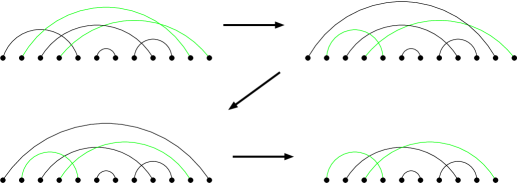
Figure 4.2. The steps of the tail-swapping bijection applied to the connected matching corresponding to the rooted map in Figure 4.1; the result is a complete matching (in the lower right) in which nonnested edges are eligible for weight $c$.

This map is a bijection because it can be reversed: given such a weighted matching on $2n$ vertices, add a new edge that nests the entire matching, and swap tails with the green edges (those of weight $c$) from right to left. Observe that the green edges in the connected matching—which are nonnested—will end up nonnested after the tail-swapping bijection, and vice versa, so this bijection is weight-preserving. Note that in the example of Figure 4.2 and subsection 4.1, the connected matching corresponded to a complete matching which was also connected. Of course this does not always happen: the connected matching $(1,5)(2,4)(3,8)(6,7)$ corresponds to the unconnected complete matching $(1,3)(2,4)(5,6)$ under this bijection.

Theorem 4.1 established that the generating functions for rooted maps and connected matchings are the same; that theorem, together with the bijection between connected matchings and arbitrary complete matchings, provides a proof of the following theorem.

Theorem 4.2.

The generating functions for rooted maps with $n$ edges, connected matchings on $2n+2$ vertices, and complete matchings on $2n$ vertices all equal the moment $\mu_{2n}(c+1)$ of the associated Hermite polynomials.

4.1. The moment generating function

Let $f(t;c)$ be the ordinary generating function for the moments of the associated Hermite polynomials:

$$f(t;c):=\sum\mu_{n}(c)t^{n}.$$

With the results of this section, we see that a continued fraction for $f(t;c)$ is implicit in [AB00, Theorem 3]: their function $M(y,z)$ counts rooted maps with the exponent of $y$ counting the number of vertices, and the exponent of $z$ counting the number of edges. We know that $\mu_{2n}(c+1)$ is the generating function for rooted maps with $n$ edges, in which all vertices except one get weight $c$, which means

(4.1) $$f(t;c+1)=\frac{M(c,t^{2})}{c}=\cfrac{1}{1-\cfrac{(c+1)t^{2}}{1-\cfrac{(c+2)t^{2}}{1-\cfrac{(c+3)t^{2}}{1-\cdots}}}}.$$

This continued fraction can also be obtained with the method of [Vie83, p. V-4], where Viennot shows a continued fraction expansion for the moment generating function for any set of orthogonal polynomials where the recurrence coefficients are known.

In the last two sections, we’ve shown bijections between the moments of the associated Hermites, connected matchings, rooted maps and oscillating tableaux. We summarize these correspondences by going all the way from a rooted map, to a connected matching, to a regular complete matching, to an oscillating tableau in subsection 4.1.

Table 1. A rooted map, a connected matching, a complete matching, and an oscillating tableau, all of weight $c^{5}$, that correspond to each other using the weight-preserving bijections of this paper. In the tableau, we have only colored the first box that corresponds to a number which gets weight $c$.

Object	What gets weight $c$
	Vertices not adjacent to head of root edge.

& Non-nested edges except edge containing vertex $1$. Non-nested edges may have weight $1$ or $c$. Numbers that appear in first column may have weight $1$ or $c$.

4.2. A second model for associated Hermite polynomials

The above discussion of connected matchings meshes nicely with a second combinatorial model of the associated Hermites, which is motivated by identity  (4.2) below. The key features of this second model are very similar to those of the connected matching model for the moments: we are using $c+1$ but there are no choices for the weights of parts of the matching, and the resulting matching is connected. The identity is found in Askey and Wimp [AW84, equation  (4.18)] and we present a combinatorial proof.

Theorem 4.3.

The associated Hermites may be written as a sum of usual Hermite polynomials:

(4.2) $$H_{n}(x;c+1)=\sum_{k\geq 0}(-1)^{k}(c)_{k}\binom{n-k}{k}H_{n-2k}(x).$$

We will need two lemmas to prove Theorem 4.3.

Lemma 4.3.

$(-1)^{k}(c)_{k}$ is the generating function for complete matchings on $2k$ vertices, with the $c+1$ associated Hermite polynomial weighting, such that all edges of weight $-1$ have a left crossing by an edge of weight $-c$. Furthermore, in such matchings there are exactly $k$ “slots” available underneath the edges weighted $-c$ where one could place the left endpoint of a new edge of weight $-1$, and only one “slot” available for the left endpoint of a new edge of weight $-c$.

Figure 4.3 shows an example of such a configuration.

Figure 4.3. A matching on $6$ vertices of the type described by subsection 4.2. If the new edge on the right is to have weight $-1$ and satisfy the conditions of the lemma, it must connect to a new vertex in one of the three available slots, indicated by the solid arrows.

Proof.

The proof goes by induction. The base cases are clear, and if true for some $k$, given any configuration for that $k$, we can either:

• add a new edge connecting vertices $2k+1$ and $2k+2$ which has weight $-c$, and hence we multiply the generating function for $2k$ vertices by $-c$ and add a new slot, or

• add a new edge from the rightmost vertex and put its left endpoint in any one of the $k$ “slots” underneath one of the $-c$ edges. Such an edge must have weight $-1$, and there are $k$ ways to place this edge, hence we effectively multiply the generating function by $k$, and since we put a new edge into one of the $k$ slots, there are now $k+1$ slots available below edges weighted $-c$.

See Figure 4.3 for an example of case 2. Altogether we’ve multiplied $(-1)^{k}(c)_{k}$, the generating function for $2k$ vertices, by $-(c+k)$, so the lemma is true by induction. ∎

Lemma 4.3.

For such a configuration on $2k$ vertices as described in subsection 4.2, there are $k+1$ places where the left endpoint of one or more green edges of weight $1$ could be placed without affecting the weight of the configuration.

Proof.

Induction again. The green edges cannot cross the $-c$ edges. For example, in Figure 4.3, there are four places where one could place such an edge, indicated by the dotted arrows. ∎

Proof of Theorem 4.3.

Since $H_{n}(x;c)$ is an even or odd polynomial if $n$ is even or odd, respectively, we can certainly write

(4.3) $$H_{n}(x;c+1)=\sum_{k\geq 0}a_{nk}H_{n-2k}(x)$$

for some coefficients $a_{nk}$. We show that those coefficients equal $(-1)^{k}(c)_{k}\binom{n-k}{k}$. Fix $k$ between $0$ and $n/2$, multiply both sides by $H_{n-2k}(x)$, and apply the usual Hermite linear functional $\mathcal{L}_{1}$. On the right side, we use orthogonality and equation (4.3) becomes

$$\mathcal{L}_{1}(H_{n}(x;c+1)H_{n-2k}(x))=a_{nk}(n-2k)!.$$

Thinking of the left side as paired matchings on $[n]$ and $[n-2k]$ with black edges of weight $-1$ and $-c$ as appropriate, and green edges all of weight $1$, we may apply the following involution: find the leftmost homogeneous edge of weight $\pm 1$ in $[n]$ or $[n-2k]$ and flip its color, unless that edge has a left crossing with an edge of weight $-c$. Swapping the colors on such edges does not preserve the weight of the paired matching.

subsection 4.2 tells us the generating function of the configurations of edges that remain in $[n]$ after applying the involution; subsection 4.2 tells us that such configurations may be viewed as consisting of $k$ “chunks” of vertices. Placing the green edges into those chunks is equivalent to forming a weak composition of $k$ into $n-2k+1$ parts; there are $\binom{n-k}{k}$ such compositions, and having chosen where the $n-2k$ edges in $[n]$ start, we can choose their endpoints in $[n-2k]$ in $(n-2k)!$ ways. Together we have

$$(-1)^{k}(c)_{k}\binom{n-k}{k}(n-2k)!=\mathcal{L}_{1}(H_{n}(x;c)H_{n-2k}(x))=a_{nk}(n-2k)!$$

which proves the identity of Theorem 4.3. ∎

The above proof relies crucially on being able to give weight $-1$ or $-c$ to edges; if we used $H_{n}(x;c)$, the above involution would not cancel as many edges, and we would need to replace subsection 4.2 with something more complicated in order to handle the $(c-1)_{k}$ factor.

Our first model for the associated Hermite polynomials (Theorem 1.1) involved incomplete matchings on $n$ vertices; the above identity motivates the following model for $H_{n}(x;c+1)$ as matchings on $n+2$ vertices.

Theorem 4.4.

The associated Hermite polynomial $H_{n}(x;c+1)$ is the generating function for certain connected incomplete matchings on $n+2$ vertices with the following weights:

• The edge containing vertex $1$ has weight $1$. Call this edge the “fake edge”.

• Fixed points have weight $x$.

• Non-nested edges (except the fake edge) have weight $-c$.

• Nested edges have weight $-1$.

In such matchings, fixed points must be nested by the fake edge. All edges other than the fake edge must either cross or be nested by the fake edge.

An example of such a matching for $H_{7}(x;c+1)$ is shown in Figure 4.4. It is clear that the requirement for nesting and crossing the fake edge yields a connected matching. Note that the connected matching moments of section 4 also have a fake edge.

Figure 4.4. A matching on $9$ vertices that contributes $cx$ to $H_{7}(x;c+1)$ using the combinatorial interpretation of Theorem 4.4. Note the “fake edge” of weight $+1$.

First proof.

Consider the $k$th term in the sum (4.2):

$$(-1)^{k}(c)_{k}\binom{n-k}{k}H_{n-2k}(x).$$

Begin with the fake edge and put $k$ vertices to the right of it. Put the remaining $n-k$ vertices underneath the fake edge and choose $k$ of them to connect with the edges that will come from the $k$ vertices on the right of the fake edge; that accounts for the binomial coefficient. On the remaining $n-2k$ vertices underneath the fake edge, we put a regular Hermite-style matching; all the edges will have weight $-1$ since they are nested by the fake edge.

The last thing to do is account for the $k$ edges that come from the right of the fake edge and show that they contribute $(-1)^{k}(c)_{k}$. According to subsection 4.2, the generating function for such a configuration with edges of weight $+1$ and $+c$ is $(c+1)_{k-1}$, but in our subset, the leftmost edge also gets weight $c$, so the correct factor is $(c+1)_{k-1}\cdot c=(c)_{k}$. Also, we must correct for the signs: our edges have weight $-1$ and $-c$, so we multiply by $(-1)^{k}$. ∎

Second proof.

Verify that the generating function described in the theorem satisfies the three-term recurrence for the associated Hermites  (1.1). We proceed very much like the usual combinatorial proof of the recurrence relation for Hermite polynomials: any such restricted matching on $n+3$ vertices may be obtained by placing the fake edge and considering the rightmost vertex nested by the fake edge. There are three possibilities: one, we can leave that vertex fixed, and fill in the remaining $n+2$ vertices with any restricted matching; two, we can add an edge from that vertex to the very rightmost vertex, and fill in the remaining $n+1$ vertices with any restricted matching; three, we can attach that vertex to any vertex except the rightmost vertex and fill in the remaining $n+1$ vertices as before. The first case contributes $x$ times the generating function for $n+2$ vertices. The second cases contributes $-c$ times the generating function for $n+1$ vertices, since that new edge cannot be nested, and it will not nest any of the other edges. In the third case, there are $n$ vertices to choose from and all of them will result in a nested edge of weight $-1$, so we add $-n$ times the generating function for $n+1$ vertices. This exposition is simply another way of stating (1.1):

$$H_{n+1}(x;c+1)=xH_{n}(x;c+1)-(n+c)H_{n-1}(x;c+1).\qed$$

The following lemma was used in the first proof of Theorem 4.4. It may be proved by induction, similar to subsection 4.2 and Theorem 1.3.

Lemma 4.4.

The generating function for complete matchings on $2n$ vertices in which all edges go from the “left $n$” vertices to the “right $n$” vertices , with all nonnested edges having weight $c$ except the edge containing the leftmost vertex, is $(c+1)_{n-1}$.

There is a weight-preserving bijection between such matchings and permutations $\pi$ of $[n]$ weighted by $c^{\,\operatorname{LRM}(\pi)-1}$ where $\operatorname{LRM}(\pi)$ is the number of left-to-right-maxima of the permutation.

At this point, we have a combinatorial interpretation for both the associated Hermite polynomials (Theorem 4.4) and their moments (Theorem 4.2) in terms of connected matchings with a fake edge; the natural thing to do is combine these to get another proof of orthogonality. This will be quite difficult because it is not at all obvious how to combine a pair of matchings for the polynomials and a matching for the moments to get a paired matching; one would have two fake edges from the polynomials and would need to somehow incorporate the fake edge from the moments into that configuration. However, it is interesting to note that the above theorem tells us how we would derive the $L^{2}$ norm using such a setup: $H_{n}(x;c)^{2}$ would be a pair of matchings on $2n+4$ vertices, but because of the extra fake edge mentioned above, after canceling all homogeneous edges we would effectively get complete matchings on $2n+2$ vertices in which all the edges go from the left $n+1$ vertices to the right $n+1$. The generating function for such a configuration, according to subsection 4.2, is $(c+1)_{n}$, which agrees with the known $L^{2}$ norm for the associated Hermites at $c+1$.

5. Unanswered questions and future directions

We have taken the basic combinatorial model in section 1 for associated Hermite polynomials and their moments and gone in two directions: to oscillating tableaux, and to rooted maps. The appeal of oscillating tableaux is in the recent flurry of work on $k$-crossings and $k$-nestings in matchings and set partitions; see [CDD⁺07, Kra06, dM07, Kla06, KZ06, Jel07]. The moments of Charlier polynomials are generating functions for set partitions and it seems likely that some of this work could be used to treat the associated Charlier polynomials.

Observe that in the connected matchings, the rooted maps, and in the second combinatorial model for the associate Hermite polynomials of Theorem 4.4, each model has some sort of “fake edge”. Combining the models for the moments and polynomials which both involve connected matchings would be interesting, but this has not yet shown promise. A major problem is that each incomplete matching for the polynomial is weighted by $x$ to the number of fixed points—say there are $2k$ fixed points—but the corresponding matchings are matchings on $2k+2$ vertices. It is not clear how to combine these two objects in a geometric or graph-theoretical way that allows a natural and easy proof of orthogonality.

Using rooted maps holds promise, though: Ossona de Mendez and Rosenstiehl have generalized the bijection between connected matchings and rooted maps to a bijection between permutations and hypermaps [OdMR04, OdMR99]. This suggests an intriguing connection to Laguerre polynomials since hypermaps are built out of permutations in the same way that maps are built out of complete matchings. The paper of Askey and Wimp [AW84] which inspired this work devotes much more attention to the associated Laguerres than to Hermites—about two thirds of the article. It is natural, then, to work out a corresponding combinatorial treatment of those polynomials, especially given the connections between rooted maps and hypermaps. There is also the work of Ismail et al. [ILV88] who work with the associated Laguerres as birth and death processes—there has been work on birth and death processes and lattice paths [FG00] which suggests another avenue for a combinatorial theory of those polynomials.

6. Acknowledgements

This work is based on part of the author’s doctoral thesis, completed at the University of Minnesota under the direction of Dennis Stanton. The author thanks Professor Stanton for his assistance and patience and the University of Minnesota math department for their support. This work was presented at FPSAC 2007 and the author thanks the FPSAC referees for their careful reading and helpful comments. Thanks also to Bill Chen and Jang Soo Kim, who helped correct some minor errors.

References

- [AB84] George E. Andrews and David M. Bressoud, Identities in combinatorics. III. Further aspects of ordered set sorting, Discrete Math. 49 (1984), no. 3, 223–236, doi:10.1016/0012-365X(84)90159-6. MR 743793.
- [AB00] Didier Arquès and Jean-François Béraud, Rooted maps on orientable surfaces, Riccati’s equation and continued fractions, Discrete Math. 215 (2000), no. 1-3, 1–12, doi:10.1016/S0012-365X(99)00197-1. MR 1746444.
- [AGV82] Ruth Azor, J. Gillis, and J. D. Victor, Combinatorial applications of Hermite polynomials, SIAM J. Math. Anal. 13 (1982), no. 5, 879–890, doi:10.1137/0513062. MR 668329.
- [And75] George E. Andrews, Identities in combinatorics. I. On sorting two ordered sets, Discrete Math. 11 (1975), 97–106, doi:10.1016/0012-365X(75)90001-1. MR 389609.
- [AW84] Richard Askey and Jet Wimp, Associated Laguerre and Hermite polynomials, Proc. Roy. Soc. Edinburgh Sect. A 96 (1984), no. 1-2, 15–37. MR 741641.
- [CDD+07] William Y. C. Chen, Eva Y. P. Deng, Rosena R. X. Du, Richard P. Stanley, and Catherine H. Yan, Crossings and nestings of matchings and partitions, Transactions of the American Mathematical Society 359 (2007), no. 4, 1555–1575, arXiv:math/0501230, doi:10.1090/S0002-9947-06-04210-3. MR 2272140.
- [dM07] Anna de Mier, -noncrossing and -nonnesting graphs and fillings of Ferrers diagrams, Combinatorica 27 (2007), no. 6, 699–720. MR 2384413.
- [dMV94] Anne de Médicis and Xavier G. Viennot, Moments des -polynômes de Laguerre et la bijection de Foata-Zeilberger, Adv. in Appl. Math. 15 (1994), no. 3, 262–304, doi:10.1006/aama.1994.1010. MR 1291053.
- [dSCV85] Myriam de Sainte-Catherine and Gérard Viennot, Combinatorial interpretation of integrals of products of Hermite, Laguerre and Tchebycheff polynomials, Orthogonal polynomials and applications (Bar-le-Duc, 1984), Lecture Notes in Math., vol. 1171, Springer, Berlin, 1985, pp. 120–128. MR 0838977.
- [FG00] Philippe Flajolet and Fabrice Guillemin, The formal theory of birth-and-death processes, lattice path combinatorics and continued fractions, Adv. in Appl. Probab. 32 (2000), no. 3, 750–778, doi:10.1239/aap/1013540243. MR 1788094.
- [FS84] Dominique Foata and Volker Strehl, Combinatorics of Laguerre polynomials, Enumeration and design (Waterloo, Ont., 1982), Academic Press, Toronto, ON, 1984, pp. 123–140. MR 782311.
- [ILV88] Mourad E. Ismail, Jean Letessier, and Galliano Valent, Linear birth and death models and associated Laguerre and Meixner polynomials, J. Approx. Theory 55 (1988), no. 3, 337–348, doi:10.1016/0021-9045(88)90100-1. MR 968940.
- [Ism05] Mourad E. H. Ismail, Classical and quantum orthogonal polynomials in one variable, Encyclopedia of Mathematics and its Applications, Cambridge University Press, November 2005. ISBN 0521782015.
- [Jel07] Vít Jelínek, Dyck paths and pattern-avoiding matchings, European J. Combin. 28 (2007), no. 1, 202–213, doi:10.1016/j.ejc.2005.07.013. MR 2261812.
- [JV00] David Jackson and Terry Visentin, An atlas of the smaller maps in orientable and nonorientable surfaces, Chapman & Hall/CRC, September 2000. ISBN 1584882077.
- [Kla06] Martin Klazar, On identities concerning the numbers of crossings and nestings of two edges in matchings, SIAM J. Discrete Math. 20 (2006), no. 4, 960–976 (electronic), doi:10.1137/050625357. MR 2272241.
- [Kra06] C. Krattenthaler, Growth diagrams, and increasing and decreasing chains in fillings of Ferrers shapes, Adv. in Appl. Math. 37 (2006), no. 3, 404–431, doi:10.1016/j.aam.2005.12.006. MR 2261181.
- [KZ06] Anisse Kasraoui and Jiang Zeng, Distribution of crossings, nestings and alignments of two edges in matchings and partitions, Electron. J. Combin. 13 (2006), no. 1. MR 2212506.
- [LY89] Jacques Labelle and Yeong N. Yeh, The combinatorics of Laguerre, Charlier, and Hermite polynomials, Stud. Appl. Math. 80 (1989), no. 1, 25–36. MR 1002302.
- [Mar94] Clemens Markett, Linearization of the product of symmetric orthogonal polynomials, Constr. Approx. 10 (1994), no. 3, 317–338, doi:10.1007/BF01212564. MR 1291053.
- [Nan58] T. S. Nanjundiah, Remark on a note of P. Turàn, Amer. Math. Monthly 65 (1958), 354–354. MR 98042.
- [OdMR99] Patrice Ossona de Mendez and Pierre Rosenstiehl, Connected permutations and hypermaps, Tech. Report 183, Centre d’Analyse et de Mathématique Sociales, July 1999, http://citeseer.ist.psu.edu/demendez99connected.html.
- [OdMR04] by same author, Transitivity and connectivity of permutations, Combinatorica 24 (2004), no. 3, 487–501, doi:10.1007/s00493-004-0029-4. MR 2085369.
- [OdMR05] by same author, Encoding pointed maps by double occurrence words, August 2005, http://hal.ccsd.cnrs.fr/ccsd-00007477.
- [Slo] N. J. A. Sloane, The on-line encyclopedia of integer sequences, http://www.research.att.com/~njas/sequences/.
- [Sun90] Sheila Sundaram, The Cauchy identity for , J. Combin. Theory Ser. A 53 (1990), no. 2, 209–238, doi:10.1016/0097-3165(90)90058-5. MR 1041446.
- [Tou52] Jacques Touchard, Sur un problème de configurations et sur les fractions continues, Canadian J. Math. 4 (1952), 2–25. MR 46325.
- [Tut73] William T. Tutte, What is a map?, New directions in the theory of graphs (Proc. Third Ann Arbor Conf., Univ. Michigan, Ann Arbor, Mich., 1971), Academic Press, New York, 1973, pp. 309–325. MR 376413.
- [Vie83] Gérard Viennot, Une théorie combinatoire des pôlynomes othogonaux generaux, Sep-Oct 1983, http://web.mac.com/xgviennot/iWeb/Xavier_Viennot/671870C1-94C7-4617-AF8%A-DE8ABFE701E3.html.
- [Vie85] by same author, A combinatorial theory for general orthogonal polynomials with extensions and applications, Orthogonal polynomials and applications (Bar-le-Duc, 1984) (Berlin), Lecture Notes in Math., vol. 1171, Springer, 1985, pp. 139–157. MR 838979.
- [Zen92] Jiang Zeng, Weighted derangements and the linearization coefficients of orthogonal Sheffer polynomials, Proc. London Math. Soc. (3) 65 (1992), no. 1, 1–22, doi:10.1112/plms/s3-65.1.1. MR 1162485.