Identification of shallow two-body bound states in finite volume

Abstract:

We discuss signatures of bound-state formation in finite volume via the Lüscher finite size method. Assuming that the phase-shift formula in this method inherits all aspects of the quantum scattering theory, we may expect that the bound-state formation induces the sign of the scattering length to be changed. If it were true, this fact provides us a distinctive identification of a shallow bound state even in finite volume through determination of whether the second lowest energy state appears just above the threshold. We also consider the bound-state pole condition in finite volume, based on Lüscher’s phase-shift formula and then find that the condition is fulfilled only in the infinite volume limit, but its modification by finite size corrections is exponentially suppressed by the spatial lattice size $L$. These theoretical considerations are also numerically checked through lattice simulations to calculate the positronium spectrum in compact scalar QED, where the short-range interaction between an electron and a positron is realized in the Higgs phase.

1 Introduction

Signatures of bound-state formation in finite volume are of main interest in this paper. In the infinite volume, the bound state is well defined since there is no continuum state below threshold. However, in a finite box on the lattice, all states have discrete energies. Even worse, the lowest energy level of the elastic scattering state appears below threshold in the case if an interaction is attractive between two particles [1]. Therefore, there is an ambiguity to distinguish between the shallow (near-threshold) bound state and the lowest scattering state in finite volume in this sense.

We may begin with a naive question: what is the legitimate definition of the shallow bound state in the quantum mechanics? In the scattering theory, poles of the $S$-matrix or the scattering amplitude correspond to bound states [2]. It is also known that the appearance of the $S$-wave bound state is accompanied by an abrupt sign change of the $S$-wave scattering length [2]. It is interpreted that formation of one bound-state raises the phase shift at threshold by $\pi$. This particular feature is generalized as Levinson’s theorem [2]. Thus, it is interesting to consider how the formation condition of bound states is implemented in Lüscher’s finite size method, which is proposed as a general method for computing low-energy scattering phases of two particles in finite volume [1].

In this paper, we discuss bound-state formation on the basis of the Lüscher’s phase-shift formula and then present our proposal for identifying the shallow bound state in finite volume. To exhibit the validity and efficiency of our proposal, we perform numerical studies of the positronium spectroscopy in compact scalar QED model. In the Higgs phase of $U(1)$ gauge dynamics, the photon is massive. Then, massive photons give rise to the short-ranged interparticle force between an electron and a positron, which is exponentially damped. In this model, we can control positronium formation in variation with the strength of the interparticle force and then explore distinctive signatures of the bound-state formation in finite volume. The contents of this paper are based on our published work [3].

2 Bound-state formation in Lüscher’s formula

In quantum scattering theory, the formation condition of bound states is implemented as a pole in the $S$-matrix or scattering amplitude. Here, an important question naturally arises as to how bound-state formation is studied through Lüscher’s phase-shift formula [1]. Intuitively, the pole condition of the $S$-matrix: $S={\rm e}^{2i\delta_{0}(p)}=\frac{\cot\delta_{0}(p)+i}{\cot\delta_{0}(p)-i}$ is expressed as

$$\cot\delta_{0}(p)=i,$$ (1)

which is satisfied at $p^{2}=-\gamma^{2}$ where positive real $\gamma$ represents the binding momentum. In fact, as we will discuss in the following, such a condition is fulfilled only in the infinite volume. However the finite-volume corrections on this pole condition are exponentially suppressed by the size of spatial extent $L$.

It was shown by Lüscher that the $S$-wave phase shift $\delta_{0}$ can be calculated by measuring the relative momentum of two particles $p$ in a finite box $L^{3}$ with a spatial size $L$ through the relation

$$\tan\delta_{0}(p)=\frac{\pi^{3/2}\sqrt{q^{2}}}{{\cal Z}_{00}(1,q^{2})}\;\;\;\;{\rm at}\;\;q=Lp_{n}/2\pi,$$ (2)

where the generalized zeta function ${\cal Z}_{00}(s,q^{2})\equiv\frac{1}{\sqrt{4\pi}}\sum_{{\bf n}\in Z^{3}}({\bf n}^{2}-q^{2})^{-s}$ is defined through analytic continuation in $s$ from the region $s>3/2$ to $s=1$ [1]. For negative $q^{2}$, an exponentially convergent expression of the zeta function ${\cal Z}_{00}(s,q^{2})$ has been derived in Ref. [4]. For $s=1$, it is given by

$${\cal Z}_{00}(1,q^{2})=-\pi^{3/2}\sqrt{-q^{2}}+\sum_{{\bf n}\in{\bf Z^{3}}}{}^{\prime}\frac{\pi^{1/2}}{2\sqrt{\bf n^{2}}}e^{-2\pi\sqrt{-q^{2}{\bf n^{2}}}},$$ (3)

where $\sum^{\prime}_{{\bf n}\in Z^{3}}$ means the summation without ${\bf n}=(0,0,0)$. We now insert Eq. (3) into Eq. (2) and then obtain the following formula, which is mathematically equivalent to Eq. (2) for negative $q^{2}$:

$$\cot\delta_{0}(p)=i+\frac{1}{2\pi i}\sum_{{\bf n}\in{Z^{3}}}{}^{\prime}\frac{1}{\sqrt{-q^{2}{\bf n}^{2}}}e^{-2\pi\sqrt{-q^{2}{\bf n}^{2}}}.$$ (4)

The second term in the r.h.s. of Eq. (4) vanishes in the limit of $q^{2}\rightarrow-\infty$. It clearly indicates that negative infinite $q^{2}$ is responsible for the bound-state formation. Therefore, in this limit, the relative momentum squared $p^{2}$ approaches $-\gamma^{2}$, which must be non-zero. Meanwhile, the negative infinite $q^{2}$ turns out to be the infinite volume limit.

According to the original paper [1], for negative $q^{2}$, we introduce the phase $\sigma_{0}(\kappa)$, which is defined by an analytic continuation of $\delta_{0}$ into the complex $p$ plane through the relation $\tan\sigma_{0}(\kappa)=-i\tan\delta_{0}(p)$, where $\kappa=-ip$. As a result, the bound-state pole condition in the infinite volume reads $\cot\sigma_{0}(\gamma)=-1$ for the binding momentum $\gamma$ [1]. Then, Eq. (4) can be rewritten in terms of the phase $\sigma_{0}$ as

$$\lim_{\kappa\rightarrow\gamma}\cot\sigma_{0}(\kappa)=-1+\sum_{\nu=1}^{\infty}\frac{N_{\nu}}{\sqrt{\nu}L\gamma}e^{-\sqrt{\nu}L\gamma}\\ =-1+\frac{6}{L\gamma}\left[e^{-L\gamma}+{\cal O}(e^{-\sqrt{2}L\gamma})\right],$$ (5)

where the factor $N_{\nu}$ is the number of integer vectors ${\bf n}\in Z^{3}$ with $\nu={\bf n}^{2}$. Therefore, it is found that although a bound-state pole condition is fulfilled only in the infinite volume limit, its modification by finite size corrections is exponentially suppressed by the spatial extent $L$ in a finite box $L^{3}$ . We can learn from Eq. (5) that “shallow bound states” are supposed to receive larger finite volume corrections than those of “tightly bound states” since the expansion parameter is scaled by the binding momentum $\gamma$.

3 Novel view from Levinson’s theorem

If the $S$-wave scattering length $a_{0}$, which is defined through $a_{0}=\lim_{p\rightarrow 0}\tan\delta_{0}(p)/p$, is sufficiently smaller than the spatial size $L$, one can make a Taylor expansion of the phase-shift formula (2) around $q^{2}=0$, and then obtain the asymptotic solution of Eq. (2). Under the condition $p^{2}\ll\mu^{2}$ where $\mu$ represents the reduced mass of two particles, the solution is given by

$$\Delta E\approx-\frac{2\pi a_{0}}{\mu L^{3}}\left[1+c_{1}\frac{a_{0}}{L}+c_{2}\left(\frac{a_{0}}{L}\right)^{2}\right]+{\cal O}(L^{-6}),$$ (6)

which corresponds to the energy shift of the lowest scattering state from the threshold energy. The coefficients are $c_{1}=-2.837297$ and $c_{2}=6.375183$ [1]. An important message is received from Eq. (6). The lowest energy level of the elastic scattering state appears below threshold ($\Delta E<0$) on the lattice if an interaction is weakly attractive ($a_{0}>0$) between two particles. This point makes it difficult to distinguish between near-threshold bound states and scattering states on the lattice.

Here, a crucial question arises: once the $S$-wave bound states are formed, what is the fate of the lowest $S$-wave scattering state? The answer to this question might provide a hint to resolve our main issue of how to distinguish between “shallow bound states” and scattering states. A naive expectation from Levinson’s theorem in quantum mechanics is that the energy shift relative to a threshold turns out to be opposite in comparison to the case where there is no bound state. Levinson’s theorem relates the elastic scattering phase shift $\delta_{l}$ for the $l$-th partial wave at zero relative momentum to the total number of bound states ($N_{l}$) in a beautiful relation $\delta_{l}(0)=N_{l}\pi$ . Therefore, if an $S$-wave bound state is formed in a given channel, the $S$-wave scattering phase shift should always be positive at low energies. This positiveness of the scattering phase shift is consistent with a consequence of the attractive interaction. Conversely, the $S$-wave scattering length may become negative ($a_{0}<0$), especially for the shallow bound-states [2]. Consequently, according to Eq. (6), possible negativeness of the scattering length gives rise to a positive energy-shift of the lowest scattering state relative to the threshold energy. In other words, the lowest scattering state is pulled up into the region above threshold. Therefore, the spectra of the scattering states quite resembles the one in the case of the repulsive interaction. If it were true, we can observe a significant difference in spectra above the threshold between the two systems: one has at least one bound state (bound system) and the other has no bound state (unbound system).

4 Numerical results

To explore signatures of bound-state formation on the lattice, we consider a bound state (positronium) between an electron and a positron in the compact QED with scalar matter [3]:

$$S_{\rm SQED}[U,\Phi,\Psi]=\beta\sum_{\rm plaq.}\left[1-\Re\{U_{x,\mu\nu}\}\right]-h\sum_{\rm link}\Re\{\Phi^{\ast}_{x}U_{x,\mu}\Phi_{x+{\mu}}\}+\sum_{\rm sites}\overline{\Psi}_{x}D_{\rm W}[U]_{x,y}\Psi_{y},$$ (7)

where $\beta=1/e^{2}$ and the constraint $|\Phi_{x}|=1$ is imposed. This action is described by the compact $U(1)$ gauge theory coupled to both scalar matter (Higgs) fields $\Phi$ and fermion (electron) fields $\Psi$. In this study, we treat the fermion fields in the quenched approximation.

Our purpose is to study the $S$-wave bound state and scattering states through Lüscher’s finite size method, which is only applied to the short-ranged interaction case. Thus, we fix $\beta=2.0$ and $h=0.6$ for the compact $U(1)$-Higgs action to simulate the Higgs phase of $U(1)$ gauge dynamics, where massive photons give rise to the short-ranged interparticle force between an electron and a positron. We generate $U(1)$ gauge configurations with a parameter set, $(\beta,h)=(2.0,0.6)$, on $L^{3}\times 32$ lattices with several spatial sizes, $L=12,16,20,24,28$ and 32. Details of our simulations are found in Ref.  [3].

Once the parameters of the compact $U(1)$-Higgs part, $(\beta,h)$, are fixed, the strength of an interparticle force between electrons should be frozen on given gauge configurations. However, if we consider the fictitious $Q$-charged electron, the interparticle force can be controlled by this charge $Q$ since the interparticle force is proportional to (charge $Q)^{2}$. Within the quenched approximation, this trick of the $Q$-charged electron is easily implemented by replacing $U(1)$ link fields as $U_{x,\mu}\longrightarrow U^{Q}_{x,\mu}=\Pi_{i=1}^{Q}U_{x,\mu}$ into the Wilson-Dirac matrix [3]. According to our previous pilot study [5], numerical simulations are performed with two parameter sets for fermion (electron) fields, $(Q,\kappa)$=(3, 0.1639) and (4, 0.2222). As we will see later, the former case ($Q=3$) corresponds to the unbound system, while the latter case ($Q=4$) corresponds to the bound system where the positronium state can be formed. Here $\kappa$, which is the hopping parameter of the Wilson-Dirac matrix, is adjusted to yield almost the same electron masses $M_{e}\approx 0.5$ for both charges.

We are especially interested in the ${}^{1}S_{0}$ and ${}^{3}S_{1}$ states of the $e^{-}e^{+}$ system, where the electron-positron bound state (positronium) could be formed even in the Higgs phase. ${}^{1}S_{0}$ and ${}^{3}S_{1}$ positronium are described by the bilinear pseudo-scalar operator $\overline{\Psi}_{x}\gamma_{5}\Psi_{x}$ and vector operator $\overline{\Psi}_{x}\gamma_{\mu}\Psi_{x}$ respectively. Therefore, we may construct the four-point functions of electron-positron states based on the above operators. We are interested in not only the lowest level of two-particle spectra, but also the 2nd and 3rd lowest levels. In order to extract a few low-lying energy levels of two-particle system, we utilize the diagonalization method [6]. We consider three types of operators for this purpose: $\Omega_{P}(t)={L^{-3}}\sum_{\bf x}{\overline{\Psi}}({\bf x},t)\Gamma\Psi({\bf x},t)$, $\Omega_{W}(t)={L^{-6}}\sum_{{\bf x},{\bf y}}{\overline{\Psi}}({\bf y},t)\Gamma\Psi({\bf x},t)$ and $\Omega_{M}(t)={L^{-6}}\sum_{{\bf x},{\bf y}}{\overline{\Psi}}({\bf y},t)\Gamma\Psi({\bf x},t)e^{i{\bf p}_{1}\cdot({\bf x}-{\bf y})}$ where ${\bf p}_{1}=\frac{2\pi}{L}(1,0,0)$ and $\Gamma=\gamma_{5}$ ($\gamma_{\mu}$) for the ${}^{1}S_{0}$ (${}^{3}S_{1}$) $e^{-}e^{+}$ state. We construct the $3\times 3$ matrix correlator from above three operators $G_{ij}(t)=\langle 0|\Omega_{i}(t)\Omega^{\dagger}_{j}(0)|0\rangle$ and then employ a diagonalization of a transfer matrix. As shown in Fig. 1, the diagonalization method with our chosen three operators successfully separates the first excited state and the second excited state from the ground state [3].

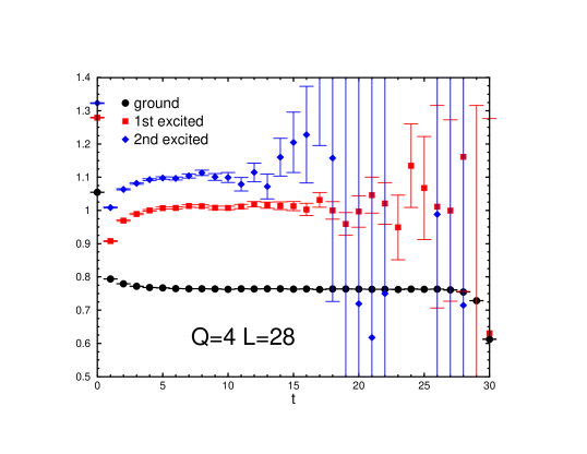
Figure 1: The effective mass plots for each eigenvalue of the transfer matrix in the ${}^{1}S_{0}$ channel on the lattice with $L=28$. Full circles, squares and diamonds represent the ground state, the first excited state and the second excited state. The left (right) panel is for $Q=3$ ($Q=4$).

4.1 Sign of energy shift

In Figs. 2, we show energies of the ground state and also excited states in the $e^{-}e^{+}$ system as a function of spatial lattice size $L$. The dashed lines and curves represent the threshold energies $2M_{e}$ and $2E_{e}({\bf p}_{1})$, which are evaluated by measured energies of the single electron with zero momentum ${\bf p}_{0}=\frac{2\pi}{L}(0,0,0)$ and nonzero lowest momenta ${\bf p}_{1}=\frac{2\pi}{L}(1,0,0)$ respectively. Two left panels are for the ${}^{1}S_{0}$ channels, while the right panel is for the ${}^{3}S_{1}$ channel.

Let us focus on results in the ${}^{1}S_{0}$ channel. The energy level of the ground state for $Q=3$ in the left panel appears close to the threshold. An upward tendency of the $L$-dependence toward the threshold energy is observed as spatial size $L$ increases. This is consistent with a behavior of the lowest scattering state predicted by Eq. (6) for the weakly attractive interaction without bound states. On the other hand, we clearly see the presence of a bound state for $Q=4$, which certainly remains finite energy gap from the threshold even in the infinite-volume limit. The most striking feature is our observed $L$-dependence of the energy level of the second lowest state for ($Q=4$). Clearly, this energy level approach the threshold energy from above. The energy shift vanishes as the spatial size $L$ increases. Therefore, the second lowest energy state must be the lowest scattering state with the repulsivelike scattering length ($a_{0}<0$). In addition, the level of the second lowest scattering state are located near and below (above) the threshold energy $2E_{e}({\bf p}_{1})$ for $Q=3$ ($Q=4$).

In the ${}^{1}S_{0}$ channel for $Q=4$, the binding energy $B$ is rather large as $B\approx M_{e}/2$. The observed bound state should be a “tightly bound state” rather than a “shallow bound state”. On the other hand, we observe that the bound state in the ${}^{3}S_{1}$ channel (the right panel) is much near the threshold energy. Although the ${}^{3}S_{1}$ ground state lies too close to the threshold energy to be assured of bound-state formation, the distinctive signature of bound state is given by an information of the excited state spectra. The second lowest state appears just above the first threshold $2M_{e}$, but far from the second threshold $2E_{e}({\bf p}_{1})$. Therefore, we can conclude: the ${}^{3}S_{1}$ ground state should be the shallow bound state, of which formation clearly induces the sign of the scattering length to change [3].

Figure 2: Energies of the ground state and excited states in the ${}^{1}S_{0}$ (the left and middle panels) and ${}^{3}S_{1}$ (the right panel) channels of the $e^{-}e^{+}$ system as functions of spatial lattice size. The left figure is for $Q=3$, while the middle and right panels are for $Q=4$.

4.2 Bound-state pole condition

A rigorous way to test for bound-state formation would be to use an asymptotic formula for finite volume correction to the pole condition as Eq. (5). In Figs.3, we plot the value of $\cot\sigma_{0}$ versus the spatial lattice extent $L$ for either ${}^{1}S_{0}$ (left) and ${}^{3}S_{1}$ (right) channels. Full circles are measured value at five different lattice volumes. At first glance, we observe that the phase $\cot\sigma_{0}$ gradually approaches $-1$ as spatial lattice extent $L$ increases for either channels.

We next examine the $L$-dependence of $\cot\sigma_{0}$ by reference to Eq. (5), where the finite volume corrections on the bound-state pole condition are theoretically predicted. The solid and dashed curves represent fit results with a single leading exponential term and three (six) exponential terms in the ${}^{1}S_{0}$ (${}^{3}S_{1}$) channel. All five data points are used for those fits in the ${}^{1}S_{0}$ channel, while the four data points in the region $20\leq L\leq 32$ are used in the ${}^{3}S_{1}$ channel. The fitting with the three (six) exponential terms yields a convergent result of $\gamma$ in the ${}^{1}S_{0}$ (${}^{3}S_{1}$) channel. Either fit curves in Figs. 3 reproduce all data points except for data at the smallest $L$ in the ${}^{3}S_{1}$ channel. Therefore, we confirm that the ground state in the ${}^{3}S_{1}$ channel at least for $L\geq 20$ can be identified as a shallow bound state without ambiguity.

Figure 3: $\cot\sigma_{0}$ in the ${}^{1}S_{0}$ (left) and ${}^{3}S_{1}$ (right) channel for $Q=4$ as a function of the spatial lattice size $L$.

5 Summary and conclusion

In this paper, we have discussed formation of an S-wave bound-state in finite volume on the basis of Lüscher’s phase-shift formula. We have first showed that although a bound-state pole condition is fulfilled only in the infinite volume limit, its modification by the finite size corrections is exponentially suppressed by the spatial extent $L$ in a finite box $L^{3}$. We have also confirmed that the appearance of the S-wave bound state is accompanied by an abrupt sign change of the S-wave scattering length even in finite volume through numerical simulations. This distinctive behavior may help us to discriminate the shallow bound state from the lowest energy level of the scattering state in finite volume simulations.

References

- [1] M. Lüscher, Commun. Math. Phys. 104, 177 (1986), Nucl. Phys. B 354, 531 (1991).
- [2] R. G. Newton, “Scattering Theory of Waves and Particles”, 2nd ed. (Springer, New York, 1982).
- [3] S. Sasaki and T. Yamazaki, Phys. Rev. D 74, 114507 (2006).
- [4] E. Elizalde, Commun. Math. Phys. 198, 83 (1998).
- [5] S. Sasaki and T. Yamazaki, PoS LAT2005, 061 (2006).
- [6] M. Lüscher and U. Wolff, Nucl. Phys. B 339, 222 (1990).