Origin of Chromatic Features in Multiple Quasars

Abstract

Aims. In some of the lensed quasars, color differences between multiple images are observed at optical/near-infrared wavelengths. There are three possible origins of the color differences: intrinsic variabilities of quasars, differential dust extinction, and quasar microlensing. We examine how these three possible scenarios can reproduce the observed chromaticity.

Methods. We evaluate how much color difference between multiple images can be reproduced by the above three possible scenarios with realistic models; (i) an empirical relation for intrinsic variabilities of quasars, (ii) empirical relations for dust extinction and theoretically predicted inhomogeneity in galaxies, or (iii) a theoretical model for quasar accretion disks and magnification patterns in the vicinity of caustics.

Results. We find that intrinsic variabilities of quasars cannot be a dominant source responsible for observed chromatic features in multiple quasars. In contrast, either dust extinction or quasar microlensing can nicely reproduce the observed color differences between multiple images in most of the lensed quasars. Taking into account the time interval between observations at different wavebands in our estimations, quasar microlensing is a more realistic scenario to reproduce the observed color differences than dust extinction. All the observed color differences presented in this paper can be explained by a combination of these two effects, but monitoring observations at multiple wavebands are necessary to disentangle these.

1 Introduction

Gravitational lensing represents a major observational tool in modern astronomy and astrophysics. Although its practical application has been mainly focused on cosmological aspects at the beginning (e.g., Zel’dovich, 1964; Refsdal, 1964; Paczyński, 1986), the subjects extend to studies of galactic structure (e.g., Oguri et al., 2002), searches for exo-planets including earth mass planets (e.g., Beaulieu et al., 2006) and others. A fundamental feature of gravitational lensing is achromaticity; this means that in principle gravitational lensing effects show no dependence on wavelength. In many situations, this achromaticity is important to discriminate gravitational lensing effects from other annoying phenomena for the detection; for instance, variable stars in galactic microlensing surveys (e.g., Alcock et al., 1996). However, some gravitational lensing phenomena are associated with unexpected chromatic features; that is, observed properties have wavelength dependence (e.g., Falco et al., 1999). In such cases, the gravitational lensing hypothesis has been confirmed using other supporting observations; studying these objects is important to obtain deeper insight into the effect of chromaticity in lensed objects.

An important example appears as the color difference between multiple images of lensed quasars. Although multiple images of lensed quasars should have the same color as the non-lensed image according to the principle of gravitational lensing, some lensed quasars show a clear color difference between different images. One possible explanation for the observed chromaticity is differential dust extinction inside the lens galaxy. It is apparent that the spatial distribution of interstellar gas and dust is inhomogeneous in galaxies. The light path of different images pass different parts of the lens galaxy, and it is natural to consider that different images are affected by spatially varying dust extinction characteristics. Within this scenario, the amount of color difference between images at given wavebands is mainly determined by three quantities: the redshift of the lens galaxy, the column density of dust, and the extinction properties of dust. Thus, we can probe these three quantities from photometric data of more than three wavebands. Falco et al. (1999) have investigated a method to probe the dust extinction in distant galaxies, Toft et al. (2000); Muñoz et al. (2004); Elíasdóttir et al. (2006); Mediavilla et al. (2005) have explored the extinction law at high-redshift galaxies, and Dai et al. (2006) have probed the dust-to-gas ratio of galaxies at cosmological distance by combining the hydrogen column density obtained with the Chandra X-ray Observatory and the color excess obtained by Falco et al. (1999). This enables us to measure the absorption properties at distant galaxies directly, and it is complement to emission-weighted measurements of dust properties. In contrast, Jean & Surdej (1998) have proposed a method to estimate the redshift of the lens galaxy under an assumption on the extinction properties. Direct detection of the emission from the lens galaxy is not necessary for this method, and it can be a strong tool to estimate redshift of faint or so-called “dark” lens galaxies.

Unfortunately, differential extinction is not the only scenario able to explain the observed chromaticity in multiple quasars. Because multiple images have different light paths, a delay in the arrival time is always present between the images. This indicates that we observe slightly different epochs of the lensed quasar at the same time via multiple images. Quasars intrinsically change not only their luminosity but also their color with time (e.g., Wilhite et al., 2005). Incorporating time delay and intrinsic color variabilities, one could explain the observed chromaticity to some degree. In addition, quasar microlensing can be yet another candidate to explain the observed chromaticity. A theoretical investigation of chromatic features of quasar microlensing has initially been made by Wambsganss & Paczyński (1991) in the case of so-called “Huchra’s lens (Q2237+0305)”. In other systems, possible evidence for chromaticity due to microlensing has been reported, for example, by Burud et al. (2002a); Nakos et al. (2005). Since there is no essential difference between Huchra’s lens and other multiple quasars, color changes due to quasar microlensing can be an origin of the observed chromaticity and can work as a contaminant in exploring dust extinction in the lens galaxy.

In summary, there are three possibilities for the chromaticity in a multiple quasar: (i) intrinsic quasar variability, (ii) differential dust extinction, and (iii) quasar microlensing. In this paper, we consider all these three possible scenarios to explain the observed chromaticity with realistic theoretical models and reliable empirical relations. We will briefly introduce the observed chromaticity in section 2. The three possible scenarios for the observed chromaticity are individually examined in sections 3, 4, and 5. Discussions about possible and realistic origin of the observed chromaticity are presented in section 6. Throughout this paper, we adopt the following cosmological parameters: $\Omega_{\rm M}=0.3$, $\Omega_{\rm\Lambda}=0.7$, and $H_{0}=70\leavevmode\nobreak\ {\rm kms^{-1}Mpc^{-1}}$ (Spergel et al., 2006).

2 Observed Chromaticity

Several observational programs for lensed quasars are currently carried out, and we here use the data taken by one of such programs, CASTLES . CASTLES provides us with photometric data of lensed quasars of high and equal quality, and the data are suitable for comparison with theoretical models and predictions. Roughly 100 lensed quasars have been listed so far, but we pick up only 25 objects whose photometric data at F160W of Hubble Space Telescope (HST) NICMOS, and at F555W and F814W of HST WFPC2 are publically available online . This sample enables us to use two independent colors to disentangle the origin of the observed chromaticity. This is useful for breaking some degeneracy which will easily occur from a single color information, for example, degeneracy between extinction properties of dust and amount of dust. Details of the sample lensed quasars and lens galaxies are summarized in Tables Origin of Chromatic Features in Multiple Quasars, and 2.

Here, we briefly summarize how the photometric data are analyzed and obtained by Lehár et al. (2000). The brightness of objects was measured by $\chi^{2}$ minimization among the observed images and models for lensed quasars and lens galaxies. A lensed quasar image is modeled by a PSF with a sharp central core (FWHM $\sim 0.1\leavevmode\nobreak\ {\rm arcsec}$) and an outer skirt of low intensity ($\leq 1\%$ of the peak intensity), and lens galaxies are modeled by an ellipsoidal exponential disk or de Vaucouleurs models. Each lensed quasar image has 3 parameters for fitting (2-dimensional position and flux), and each lens has 6 parameters for fitting (2-dimensional position, flux, major axis, axis ratio, position angle of major axis). Uncertainties of these decomposition procedures are included in errors presented in Tables Origin of Chromatic Features in Multiple Quasars, and 2.

Table 2: Summary of lens galaxies in the current sample. Their magnitude and error at F160W, at F555W and at F814W are presented. All the data are taken from CASTLES web page. Types of the lens galaxies indicated by their spectrum, color or brightness profile are also shown. Early and late type is presented by ‘E’ and ‘L’, respectively. For a sample with two lens galaxies, they are denoted by G and G’. References. (1) Lehár et al. 2000; (2) Tonry & Kochanek 1999; (3) Fassnacht & Cohen 1998; (4) Keeton et al. 1998; (5) Burud et al. 1998; (6) Lubin et al. 2000; (7) Young et al. 1980; (8) Angonin-Willaime et al. 1994; (9) Kochanek et al. 2000; (10) Remy et al. 1998; (11) Impey et al. 1998; (12) Impey et al. 1996; (13) Chavushyan et al. 1997; (14) Koopmans & Treu 2002; (15) Fassnacht et al. 1999; (16) Lopez et al. 1998; (17) Huchra et al. 1985.

Object Name	$m_{F160W}$	$m_{F555W}$	$m_{F814W}$	Galaxy Type
				Spectrum	Color	Profile
Q0142-100 G	$16.63\pm 0.03$	$20.81\pm 0.02$	$18.72\pm 0.05$	-	E(1)	E(1)
B0218+357 G	$17.50\pm 0.04$	$21.95\pm 0.24$	$20.06\pm 0.14$	-	L(1), E(1)	L(1)
MG0414+0534 G	$17.54\pm 0.14$	$24.17\pm 0.15$	$20.91\pm 0.05$	-	E(2)	-
B0712+472 G	$17.16\pm 0.15$	$21.75\pm 0.10$	$19.56\pm 0.07$	E(3)	E(4)	-
RXJ0911+0551 G	$17.93\pm 0.08$	$22.97\pm 0.22$	$20.47\pm 0.09$	-	-	E(5), L(5)
SBS0909+523 G	$16.75\pm 0.74$	$18.29\pm 0.55$	$17.12\pm 1.12$	E(6)	E(1)	-
BRI0952-0115 G	$18.95\pm 0.16$	$23.67\pm 0.08$	$21.21\pm 0.04$	-	E(4)	E(1)
Q0957+561 G	$15.14\pm 0.09$	$19.05\pm 0.06$	$17.12\pm 0.03$	-	E(4)	E(7)
G’	$17.92\pm 0.04$	$21.87\pm 0.25$	$19.99\pm 0.24$	E(8)	-	-
LBQS1009-0252 G	$19.30\pm 0.12$	$24.05\pm 0.54$	$21.99\pm 0.04$	-	-	E(1)
B1030+071 G	$17.64\pm 0.15$	$22.71\pm 0.12$	$20.24\pm 0.13$	E(3)	E(1)	E(1)
G’	$19.11\pm 0.08$	$24.56\pm 0.20$	$22.04\pm 0.13$	-	E(1)	L(1)
HE1104-1805 G	$17.47\pm 0.27$	$23.14\pm 0.58$	$20.01\pm 0.10$	-	E(9,10)	-
PG1115+080 G	$16.66\pm 0.04$	$20.74\pm 0.04$	$18.92\pm 0.02$	-	E(4)	E(11)
B1422+231 G	$17.57\pm 0.20$	$21.80\pm 0.17$	$19.66\pm 0.25$	-	E(12)	-
SBS1520+530 G	$17.84\pm 0.06$	$21.96\pm 1.24$	$20.16\pm 0.13$	-	L(13)	-
B1600+434 G	$18.30\pm 0.13$	—	$20.78\pm 0.41$	L(4)	-	-
MG2016+112 G	$18.46\pm 0.09$	$25.12\pm 1.06$	$21.95\pm 0.09$	-	-	E(14)
G’	$23.08\pm 0.62$	$24.92\pm 0.30$	$24.56\pm 0.09$	-	-	-
B2045+265 G	$18.25\pm 0.26$	$23.86\pm 0.22$	$21.15\pm 0.19$	L(15)	-	-
HE2149-2745 G	$17.61\pm 0.10$	$21.18\pm 0.09$	$19.56\pm 0.03$	-	-	E(16)
Q2237+0305 G	$12.22\pm 0.22$	$15.49\pm 0.22$	$14.15\pm 0.20$	E(17)	-	L(17)
QJ0158-4325 G	$19.75\pm 0.27$	$22.96\pm 0.22$	$22.42\pm 0.83$	-	-	-
APM08279+5255 G	$15.11\pm 0.04$	$18.70\pm 0.07$	$16.93\pm 0.05$	-	-	-
FBQ0951+2635 G	$17.86\pm 0.23$	$21.02\pm 0.20$	$19.67\pm 0.23$	-	-	-
G’	$18.50\pm 0.30$	$20.06\pm 0.38$	$20.33\pm 0.17$	-	-	-
Q1017-207 G	$19.26\pm 0.06$	$25.48\pm 0.73$	$21.82\pm 0.48$	-	E(9)	E(1)
Q1208+101 G	—	—	—	-	-	-
FBQ1633+3134 G	$16.80\pm 1.10$	$19.21\pm 3.38$	$18.26\pm 0.89$	-	-	-

Figure 1: The lens redshift ($z_{l}$) and the source redshift ($z_{s}$) of the current samples are presented by the filled circles in this figure. Objects without the lens redshift are indicated by the filled squares with arrows.

The redshifts of the lens ($z_{l}$) and the source ($z_{s}$) listed in Tables Origin of Chromatic Features in Multiple Quasars are also taken from CASTLES, and presented in Figure 1. The redshifts of all the lensed quasars are known as presented in Tables Origin of Chromatic Features in Multiple Quasars. In contrast, the redshifts of the lens galaxies are not known in all cases. Objects with unknown redshifts or with tentative redshifts are listed at the bottom of Table Origin of Chromatic Features in Multiple Quasars. For these objects, the upper limits of their lens redshifts are set to be the source redshifts and are denoted by the filled squares with arrows in Figure 1. The source quasars and the lens galaxies are distributed at $z\simeq 1$–$4$ and at $z\simeq 0$–$1$, respectively . In total, now we have 25 objects (or 40 image pairs) for our current purpose.

In Table Origin of Chromatic Features in Multiple Quasars, the colors of each lensed quasar image for F555W – F160W and F814W – F160W, and the F160W magnitudes of each image are also presented together with their errors. The errors are evaluated in the usual manner, namely by calculating the square root of the sum of the squares of the individual error. It is apparent from Table Origin of Chromatic Features in Multiple Quasars that some of the lensed quasars show color differences between different images. This feature can also be found more clearly in Figure 2; the color differences of multiple images relative to that of the brightest image at F160W, $\Delta(m_{F555W}-m_{F160W})$ and $\Delta(m_{F814W}-m_{F160W})$. Images located at the lower left part in Figure 2 are relatively bluer than the brightest image at F160W in the system. Gravitational lensing effect has no wavelength dependence in principle, and the magnification factor should be the same at different wavebands. Since the magnitude differences between images correspond to the ratio of magnification factors only if the macro lensing contributes to the magnification, the magnitude difference should be identical among any wavebands. That is, observational data points should be located at the origin, $(0,0)$, in Figure 2 within the error. Though some of the multiple quasars show achromaticity as expected, others show anomalous chromaticity; i.e., some data points in Figure 2 significantly deviate from the origin, ranging up to $\sim 2\leavevmode\nobreak\ {\rm mag}$.

Although there is a wavelength overlap among these two combinations of the color differences, F555W – F160W and F814W – F160W, we choose these combinations because of their small errors compared to combinations of F555W – F814W. The lower-left to upper-right trend of observational data points in Figure 2 or following similar figures is a natural consequence of the wavelength overlap, and hereafter we just focus on deviations of observational data from the expected values of our calculations rather than the trend.

Figure 2: Color differences between multiple images are plotted with error bars. For each system, the brightest image in F160W has been used as color reference. The abscissa and ordinate represent the color difference derived from F555W and F160W ($\Delta(m_{F555W}-m_{F160W})$), and that from F814W and F160W ($\Delta(m_{F814W}-m_{F160W})$), respectively. Panel (a) is for lensed quasars for which the redshift of the lens galaxy is known, while Panel (b) is for lensed quasars for which the redshift of the lens galaxy is unknown.

Here, we review what kind of effect should be included for interpretation of the observed chromaticity. By using the intrinsic magnitude of a quasar ($m_{\rm int}$), the expected magnitude of an image of multiple quasars ($m_{\rm obs}$) at wavelength ($\lambda$) at any given time ($t$) is written as follows:

$$m_{\rm obs}(\lambda,t)=m_{\rm int}(\lambda,t-\tau)+A\left(\frac{\lambda}{1+z_{l}}\right)-2.5\log\left[\mu(\lambda,t)\right],$$ (1)

where $\tau$, $A$, and $\mu$ indicate the arrival time delay due to gravitational lensing, the extinction along a path from the source to observer, and the magnification due to gravitational lensing, respectively. To include the finite source size effect, as is different from a usual expression, the magnification due to gravitational lensing is presented as a function of wavelength and time in equation 1 (see section 5 for more details). These three terms all affect the multiple images with different magnitudes for different images. Thus, they can be possible origins of the observed chromaticity. In the following three sections, we examine how these effects may produce the observed chromaticity.

3 Intrinsic Variabilities of Quasars

It is well known that quasars show temporal flux variabilities at any wavebands, and the color becomes bluer when the flux gets brighter (e.g., Wilhite et al., 2005; Cristiani et al., 1997). This means that the color of quasars changes with time according to the flux variabilities. Additionally, the arrival time delay due to gravitational lensing is different at different images. This produces the relative time delay between multiple images of the same quasar, and multiple images observed at the same epoch correspond to images at intrinsically different epochs. Therefore, it is probable that multiple images observed at the same time show different colors. To estimate this effect, we evaluate typical time delays between images and typical color change of quasars for a given time interval.

Though the actual time delay is determined by the density profile of the lens galaxy, the location of the source respective to the lens on the sky, the source redshift, and the lens redshift, we can roughly evaluate the typical time delay from observed properties of multiple quasars. By assuming that the density profile of a lens galaxy is approximated by a singular isothermal sphere (SIS; e.g., Schneider et al., 1992), the time delay between two images, one image with positive parity (located at $\theta_{+}$ from the lens galaxy) and another image with negative parity (located at $\theta_{-}$ from the lens galaxy), is expressed by

$$\tau = \frac{1+z_{l}}{2c}\frac{D_{ol}D_{os}}{D_{ls}}\left(\theta_{+}^{2}-\theta_{-}^{2}\right)$$ (2)

$$= 30\left(\frac{1+z_{l}}{2}\right)\left(\frac{D_{ol}D_{os}/D_{ls}}{1\leavevmode\nobreak\ {\rm Gpc}}\right)\left(\frac{\theta_{+}^{2}-\theta_{-}^{2}}{1\leavevmode\nobreak\ {\rm arcsec}^{2}}\right)\leavevmode\nobreak\ {\rm days},$$

where $D_{ol}$, $D_{os}$, and $D_{ls}$ represent the angular diameter distances from observer to the lens, from observer to the source, and from the lens to the source, respectively. Since the image separation is on the order of $1\leavevmode\nobreak\ {\rm arcsec}$ in most multiple quasars, we can roughly estimate $\theta_{+}^{2}-\theta_{-}^{2}$ to be $\sim 1\leavevmode\nobreak\ {\rm arcsec}^{2}$. Thus, we adopt $30\leavevmode\nobreak\ {\rm days}$ for a typical time delay between multiple images.

Further, by using recent studies of intrinsic variabilities of quasars, we can also evaluate the color change of quasars on any given timescale. Vanden Berk et al. (2004); Ivezić et al. (2004) have investigated how quasar variabilities in the rest-frame optical/UV regime depend on other observational quantities such as rest-frame time lag. They analyzed relations among these quantities and the structure function a commonly used statistical measure for variabilities; e.g., Kawaguchi et al., 1998 by using imaging data of quasars obtained by Sloan Digital Sky Survey. The resulting structure function ($V$) is expressed as

$$V=\left(1+0.024M_{i}\right)\left(\frac{\Delta t_{\rm RF}}{\lambda_{\rm RF}}\right)^{0.3}\leavevmode\nobreak\ {\rm mag},$$ (3)

where $M_{i}$, $\Delta t_{\rm RF}$, and $\lambda_{\rm RF}$ represent the $i$ band absolute magnitude of a quasar in units of magnitude, the rest-frame time lag between observations in units of days, and the rest-frame wavelength in units of Å, respectively. Equation 3 indicates that a larger flux change of quasars occurs at fainter quasars, at longer time lag, and/or at shorter wavelength. The absolute $i$ band magnitude of the quasar sample is distributed from $\sim-21$ to $\sim-30$ (Vanden Berk et al., 2004). Since $\Delta t_{\rm RF}$ and $\lambda_{\rm RF}$ have the same redshift dependence, both of these quantities can be replaced by the observer-frame quantities.

Substituting the typical time delay above (30 days) and the effective wavelength of each filter into equation 3, we obtain the expected flux variation of quasars. The expected values for magnitude difference ($\delta m$) with a time lag of $30\leavevmode\nobreak\ {\rm days}$ is 0.043 – 0.075 mag, 0.059 – 0.105 mag, and 0.053 – 0.093 mag at F160W (mean wavelength: $16071$ Å), F555W (mean wavelength: $5337$ Å), and F814W (mean wavelength: $7900$ Å), respectively. Here, the maximum and the minimum value of magnitude differences are obtained for $M_{i}=-21$ and $M_{i}=-30$, respectively. Even if we take into account filter responses, these values would not change much. The wavelength coverage of all the filters is less than $\sim\pm 20\%$ of the wavelength center (see also the upper panel of Figure 4), and the expected flux variations are less than $\pm 7\%$ from the above values within the coverage (see equation 3). By comparing these expected values for magnitude difference at different wavebands, we are able to estimate the possible range of the expected color differences.

In general, the range of the expected color difference between two images for two bands labeled with $j$ and $k$, $|\Delta(m_{j}-m_{k})|$, is estimated by $||\delta m_{j}|-|\delta m_{k}||<|\Delta(m_{j}-m_{k})|<|\delta m_{j}|+|\delta m_{k}|$. The maximum value corresponds to the case where variabilities in band $j$ and that in band $k$ have completely negative correlation, i.e., when a quasar gets brighter in band $j$, a quasar always gets fainter in a $k$ band. The minimum value corresponds to the case where variabilities in these two bands have completely positive correlation, i.e., when a quasar becomes brighter in band $j$, it always gets brighter also in band $k$. For quasars with $M_{i}=-21$, the fainter end of the sample of Vanden Berk et al. (2004), the expected color differences are ranging from $|0.105-0.075|=0.030$ mag to $0.105+0.075=0.180$ mag for $|\Delta(m_{\rm F555W}-m_{\rm F160W})|$, and from $|0.093-0.075|=0.018$ mag to $0.093+0.075=0.168$ mag for $|\Delta(m_{\rm F814W}-m_{\rm F160W})|$. Since the observed chromaticities as shown in Figure 2 have values up to $\sim 2\leavevmode\nobreak\ {\rm mag}$, it is impossible to reproduce all the observed chromaticity only by this scenario which is able to reproduce a color difference up to $0.2\leavevmode\nobreak\ {\rm mag}$. For intrinsically brighter quasars, the expected flux change within a time interval is rather small, and the expected color differences are smaller than the observed values. Moreover, quasar variabilities at any two wavebands presumably have positive correlation with each other rather than a negative correlation (e.g., Wilhite et al., 2005), and the actual color difference should be smaller than our estimated maximum values.

Of course, such positive correlation will be lost if observations for an object at different wavebands are carried out at different times. Denoting this observational interval among two bands (labeled with $j$ and $k$) as $t_{lag}$, the color difference including time delay ($\tau$) is expressed as $\Delta(m_{j}-m_{k})=\left[m_{j}(t)-m_{k}(t+t_{lag})\right]-\left[m_{j}(t+\tau)-m_{k}(t+\tau+t_{lag})\right]=\left[m_{j}(t)-m_{j}(t+\tau)\right]-\left[m_{k}(t+t_{lag})-m_{k}(t+\tau+t_{lag})\right]$. This relation indicates that the expected color differences are a simple combination of magnitude differences at each band adopted above. Since an actual time delay is nothing to do with the observational interval among different wavebands, $t_{lag}$ is the only factor that makes difference from the previous situation, i.e., without the observational interval. As presented by Lehár et al. (2000), the observational interval among different wavebands spanned up to $t_{lag}\sim 2$ years for some objects, and it is comparable to maximum timescale of quasar variabilities (e.g., Ivezić et al., 2004) . Since physical correlation could be lost after a timescale longer than maximum timescale of quasar variability, a completely negative correlation among two wavebands is even possible when the observational interval is comparable to or longer than $\sim 2$ years. However, even if it is the case, the amplitude of variations estimated above fixes upper bounds on the expected color differences, and it is impossible to produce color differences larger than $|\Delta(m_{\rm F555W}-m_{\rm F160W})|=0.180{\rm\leavevmode\nobreak\ mag}$ and $|\Delta(m_{\rm F814W}-m_{\rm F160W})|=0.168{\rm\leavevmode\nobreak\ mag}$. Thus, the expected color differences should be still within the range estimated above, and thus the observed color differences cannot be explained by intrinsic variabilities of quasars alone.

The model for the lens galaxies that we used here for estimating the time delay between multiple images is rather simple, though the time delay depends on the applied lens model. This has already been mentioned in previous studies (e.g., Oguri et al., 2002), and the expected time delay of more realistic lens models can be reduced down to an order of magnitude from that of SIS. Diversity of the expected time delay is also investigated by different approaches (e.g., Saha et al., 2006), and the time delay range would be typically between $\sim 10$ and $\sim 300$ days. Further, if the lens redshift is unknown, the expected time delay of any lens model can have a dispersion of one order of magnitude for a given image separation. Consequently, taking a more realistic lens model into account, the expected time delay can change up to two orders of magnitude. Even if this is the case, the expected color difference between multiple images can change only by a factor of 4 (see equation 3).

From the observational point of view, the measured time delay shows wide variety as predicted by the previous theoretical studies (e.g., Oguri et al., 2002; Saha et al., 2006), and the measured values are different from $30\leavevmode\nobreak\ {\rm days}$. In Table 3, we summarize the time delay between multiple images in the current sample. The time delay of objects which are not listed in Table 3, Q0142-100, MG0414+0534, B0712+472, SBS0909+523, LBQS1009-0252, B1030+071, MG2016+112, B2045+265, Q2237+0305, QJ0158-4325, APM08279+5255, BRI0952-0115, Q1017-207, Q1208+101, and FBQ1633+3134, has not been successfully measured yet. As we can see in Table 3, some multiple quasars have one order of magnitude longer time delay than the typical value applied here (e.g., Kundic et al., 1997). In such systems, of course, the expected flux change is larger than that we estimated for multiple quasars with the time delay of $30\leavevmode\nobreak\ {\rm days}$. However, the color difference becomes only twice the value estimated above (see equation 3), and the observed color differences are not still explained. Again, it is clear that intrinsic variabilities of quasars alone cannot reproduce observed color difference between multiple images.

Table 3: Time delay between multiple images in current sample is presented in units of day. Wavebands used for the measurement are also presented with the reference. Only objects with the available time delay are listed here. References. (1) Biggs et al. 1999; (2) Hjorth et al. 2002; (3) Ullán et al. 2006; (4) Kundic et al. 1997; (5) Haarsma et al. 1999; (6) Ofek & Maoz 2003; (7) Schechter et al. 1997; (8) Patnaik & Narasimha 2001; (9) Burud et al. 2002b; (10) Koopmans et al. 2000; (11) Burud et al. 2002a; (12) Jakobsson et al. 2005.

Object and Image Pair	Optical Delay	Waveband	Radio Delay	Waveband
	(day)		(day)
B0218+357 A–B	—		$10.5\pm 0.4$	8.4 and 15 GHz (1)
RXJ0911+0551 A–B	$146\pm 8$	I-band (2)	—
SBS0909+523 A–B	$45^{+1}_{-11}$	R-band (3)	—
Q0957+561 A–B	$417^{+3}_{-3}$	g-band (4)	$459^{+12}_{-15}$	6 cm (5)
	$420^{+6}_{-9}$	r-band (4)	$397^{+12}_{-12}$	4 cm (5)
HE1104-1805 A–B	$161^{+7}_{-7}$	V- and R-band (6)	—
PG1115+080 A–C	$9.4$	V-band (7)	—
C–B	$23.7\pm 3.4$	V-band (7)	—
B1422+231 A–B	—		$1.5\pm 1.4$	8.4 and 15 GHz (8)
A–C	—		$7.6\pm 2.5$	8.4 and 15 GHz (8)
B–C	—		$8.2\pm 2.0$	8.4 and 15 GHz (8)
SBS1520+530 A–B	$130\pm 3$	R-band (9)	—
B1600+434 A–B	—		$47^{+5}_{-6}$	8.5 GHz (10)
HE2149-2745 A–B	$103\pm 12$	V- and i-band (11)	—
FBQ0951+2635 A–B	$16\pm 2$	R-band (12)	—

4 Differential Dust Extinction

The light paths of different images intersect different positions of the lens galaxy. In general, the column density of gas and dust along different lines of sight differs in all galaxies, and different images experience different levels of dust extinction. We can also consider that the shape of extinction curve is different at different positions in the lens galaxy. For simplicity, however, we basically take into account only the inhomogeneity of dust column densities, but we also examine the difference among various empirical extinction curves derived from the Milky Way (MW) and the Small Magellanic Cloud (SMC).

We here apply an extinction law derived for the MW dust by Cardelli et al. (1989). In this extinction law, dust extinction is characterized basically by two parameters; $A_{V}$, dust extinction at $V$ band which reflects amount of dust, and $R_{V}$ [$\equiv A_{V}/E_{B-V}$ ($E_{B-V}$ is the $B-V$ color excess)]. Since $A_{V}$ is physically related to the column density of dust, we can estimate the differential dust extinction from differential column densities of gas by assuming values of the dust-to-gas ratio and $R_{V}$. In order to obtain differential column densities of gas, we utilize a 2-dimensional galactic-scale hydrodynamical simulation presented by Hirashita et al. (2003), who adopt the calculation code of Wada & Norman (2001). The result clearly shows a clumpy distribution of gas in the simulated galaxy. The cumulative probability distribution of differential column densities, $\Delta N_{\rm H}$, is shown in Figure 3; we randomly select $10^{6}$ pairs of columns on the 2-dimensional grid points in the simulated galaxy, and derive the probability distribution function of the difference of gas column densities between each pair . As we can see from Figure 3, the expected differential column density from the simulation spans a large range: The median value is $\sim 3\times 10^{20}\leavevmode\nobreak\ {\rm cm^{-2}}$, and $90\%$ of data is distributed from $\sim 6\times 10^{18}\leavevmode\nobreak\ {\rm cm^{-2}}$ to $\sim 7\times 10^{21}\leavevmode\nobreak\ {\rm cm^{-2}}$. We apply the MW dust-to-gas ratio provided by Bohlin et al. (1978), and obtain $A_{V}=R_{V}\times E_{B-V}=3.1\times N_{\rm H}/(5.8\times 10^{21})=5.3\times 10^{-22}N_{\rm H}$, where $N_{\rm H}$ is the hydrogen column density in ${\rm cm^{-2}}$. In this paper, we apply the above relation also when we adopt values for $R_{V}$ other than 3.1. We then can convert the expected differential column densities into the expected differential extinction in the $V$ band, $\Delta A_{V}$. This conversion is fairly simple and the scale for this value is also denoted in Figure 3. The corresponding values of $\Delta A_{V}$ for the median, $5\%$, and $95\%$ of Figure 3 are $\sim 0.1\leavevmode\nobreak\ {\rm mag}$, $\sim 3\times 10^{-3}\leavevmode\nobreak\ {\rm mag}$, and $\sim 3\leavevmode\nobreak\ {\rm mag}$, respectively.

Figure 3: Cumulative probability distribution of differential column densities of gas obtained from Hirashita et al. (2003). The lower abscissa indicates the differential column density of gas in units of ${\rm cm^{-2}}$. The corresponding differential extinction at $V$ band (in mag) is also denoted at the upper abscissa. Cumulative probabilities of $5\%$, $50\%$ and $95\%$ are indicated by the dashed lines.

Additionally, it is well known that the SMC exhibits a very different extinction curve compared to the MW curve. The SMC curve lacks the 2175 Å bump and rises steeply toward shorter wavelengths in the UV. We also adopt an SMC extinction curve in the current study. Several types of the SMC extinction curves have been provided, but we investigate the extinction law by using an observational data of Gordon et al. (2003) (see appendix for details) which covers a relatively wide wavelength range. Some examples of the extinction curves that we adopted in this study are shown in Figure 4. Since Cardelli et al. (1989) have presented the extinction law only for $R_{V}=2.6-5.6$, and since there is no guarantee that the empirical extinction law is valid for $R_{V}<2.6$ or $R_{V}>5.6$, we put in this paper the same limit as Cardelli et al. (1989).

Figure 4: Extinction curves for several parameter sets (lower panel) and filter responses (upper panel) are presented. In the lower panel, the solid, the dotted, the dashed, and the long-dashed lines correspond to the extinction curve of the SMC with $N_{\rm H}=10^{21}\leavevmode\nobreak\ {\rm cm^{-2}}$, that of the MW with $N_{\rm H}=10^{21}\leavevmode\nobreak\ {\rm cm^{-2}}$ and $R_{V}=5.6$, that of the MW with $N_{\rm H}=10^{21}\leavevmode\nobreak\ {\rm cm^{-2}}$ and $R_{V}=3.1$, and that of the MW with $N_{\rm H}=3\times 10^{21}\leavevmode\nobreak\ {\rm cm^{-2}}$ and $R_{V}=3.1$, respectively. In the upper panel, filter responses for F555W, F814W, and F160W are presented by the dotted, the dashed, and the solid lines, respectively. The abscissa of the lower panel is the wavelength at the rest frame of the absorber (or the lens galaxy) in units of Å, and that of upper panel is the wavelength at observer’s frame.

Denoting the response of the filter $k$ and the spectrum of the source as $f_{k}(\lambda)$ and $S(\lambda)$, respectively, the expected magnitude at filter $k$, $m_{k}$, including dust extinction is expressed as

$$m_{k}(N_{\rm H})=m_{int,k}-2.5\log\left[\frac{\int_{\lambda_{\rm min}}^{\lambda_{\rm max}}10^{-0.4A\left[N_{\rm H},\lambda/(1+z_{l})\right]}f_{k}(\lambda)S(\lambda)\,d\lambda}{\int_{\lambda_{\rm min}}^{\lambda_{\rm max}}f_{k}(\lambda)S(\lambda)\,d\lambda}\right],$$ (4)

where $\lambda_{\rm max}$ and $\lambda_{\rm min}$ represent the maximum and minimum wavelengths of the filter response, respectively, and $m_{int,k}$ is the source magnitude without dust extinction. Finally, the expected magnitude difference between multiple images at filter $k$, $\Delta m_{k}$, due to differential dust extinction is expressed as

$$\Delta m_{k}=m_{k}(N_{\rm H})-m_{k}(N_{\rm H}^{\prime}),$$ (5)

where $N_{\rm H}$ and $N_{\rm H}^{\prime}$ are the gas column density on one image and that on the other image, and the difference of these two quantities is $\Delta N_{\rm H}$. Consequently, the expected color difference between multiple images is estimated by subtracting the magnitude difference of one filter from that of the other filter, i.e., $\Delta m_{k}-\Delta m_{j}$. Although the spectral shape of the source is clearly involved in equation 4, dependence on the assumed spectral shape causes a difference of only a few percent . Thus, we assume a flat spectrum, i.e., $S(\lambda)=\mbox{const}$. Applying equation 4 to all the filters, we can estimate the expected color differences due to differential dust extinction. The results are presented in Figure 5.

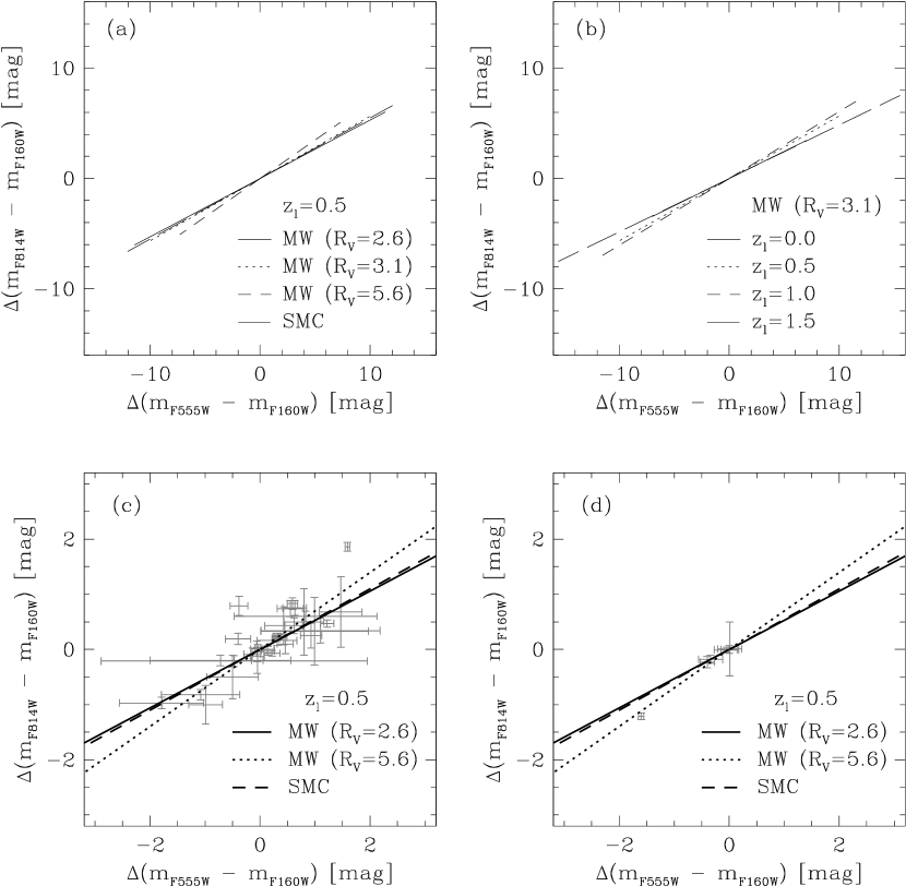
Figure 5: The upper two panels show the expected color differences between multiple images for various extinction laws at the same lens redshift (panel a), and for the same extinction law at various lens redshifts (panel b). All of these lines are drawn up to the expected color differences for $95\%$ of the cumulative differential column density of the gas in the lens galaxy, $\Delta N_{\rm H}\sim 7.1\times 10^{21}\leavevmode\nobreak\ {\rm cm^{-2}}$. In the upper left panel (panel a), the expected color differences for the MW extinction curve with $R_{V}=2.6$, with $R_{V}=3.1$, and with $R_{V}=5.6$, and for the SMC extinction curve are presented by the solid, dotted, dashed, and long-dashed lines, respectively. The applied redshift for the lens in these estimations is $0.5$. In the upper right panel (panel b), the expected color difference in the case of the lens galaxy at $z_{l}=0.0$, $0.5$, $1.0$, and $1.5$ are presented by the solid, dotted, dashed, and long-dashed lines, respectively. The applied extinction law in this estimation is the MW one with $R_{V}=3.1$, or a standard extinction law in our galaxy. The lower two panels show the expected color differences for the various extinction laws at the lens redshift of $z_{l}=0.5$. The extinction law for the MW with $R_{V}=2.6$, the MW with $R_{V}=5.6$, and the SMC are presented by the solid, dotted, and dashed lines respectively. The observational data which were shown in Figure 2 (a) and (b) is overlaid as the gray crosses in panels (c) and (d), respectively. Note that the scale of the abscissa and ordinate in the upper panels is different from that in the lower panels.

As clearly seen in Figure 5, the differential dust extinction of $95\%$ level (see Figure 3) can produce up to $\sim 10\leavevmode\nobreak\ {\rm mag}$ of color difference between multiple images of lensed quasars . The expected color difference is large enough to reproduce the observed chromaticity. Moreover, the slope nicely reproduces the observational data. We note that the above theoretical predictions do not depend strongly on the lens redshift and the applied extinction laws (see Figure 5). However, the expected color difference can be as large as a few magnitudes, exceeding the observed values for the color difference. This may be because we have adopted the simulation of a relatively gas-rich galaxy that has not yet converted a substantial fraction of the gas mass into stars (Hirashita et al., 2003). Actually, many lens galaxies are suggested to be early type galaxies, and the dust amount and distribution in such galaxies must differ from what we have applied here. In this respect, our approach may be too simplistic.

In the lower panels of Figure 5, some of the expected color differences are presented together with the same observational data as those in Figure 2 for comparison. Most of the observational data in both of these panels (panels c and d are respectively for lensed quasars whose redshift of the lens galaxy is known and unknown) are consistent with the the expected color differences within the $1\sigma$ error bar. This indicates that the observed chromaticity can be explained by differential dust extinction. However, some data points cannot be reproduced by the currently applied extinction laws. For example, an upper right data point in panel (c) has error bars small enough to conclude that it deviates significantly from the theoretical lines. We will further discuss such data points in section 6.

Here, we have applied only well-known empirical formulae for the extinction laws, and have not assumed any special, eccentric, or other unrealistic extinction laws. If it is confirmed that the differential dust extinction is responsible for the chromaticity of the lensed quasars, and if our assumption that the shape of extinction curve is the same at different positions in the lens galaxy, is valid (see, McGough et al., 2005), we can conclude that any special extinction laws are not required to reproduce dust extinction in galaxies up to $z\sim 1$, and the normal extinction laws that we have used in this study, i.e., the extinction laws derived from the local Universe, can be applicable in such distant galaxies.

5 Quasar Microlensing

From macro lensing modeling, the surface mass density of the lens divided by the critical surface mass density for lensing (e.g., Schneider et al., 1992) is of order unity for all multiple images of lensed quasars. This indicates that the probability of quasar microlensing is high enough to be observed if the mass is dominated by compact components such as stars, planets or other compact objects. As investigated by Wambsganss & Paczyński (1991), quasar microlensing can change the observed color of quasars from their intrinsic one, and $\mu(t)$ in equation 1 is also a function of wavelength. This effect has been examined by using more realistic models for quasar accretion disks (e.g., Yonehara et al., 1998). Since the spatial distribution of lens objects on different images is generally different, quasar microlensing occurs in different ways in different images and consequently the color differences may be produced by quasar microlensing. Possible microlensing signals in the observed quasar sample are summarized in appendix B.

Furthermore, the timescale of quasar microlensing can be estimated by a timescale on which the source crosses the Einstein ring radius ($t_{E}$) or a timescale on which the caustic crosses the source ($t_{c}$). The former timescale is evaluated by

$$t_{E} = \frac{r_{E}}{v_{t}}$$ (6)

$$= \frac{1}{v_{t}}\left(\frac{4GM_{\rm lens}}{c^{2}}\frac{D_{ls}D_{ol}}{D_{os}}\right)^{1/2}$$

$$\simeq 14\left(\frac{v_{t}}{10^{3}\leavevmode\nobreak\ {\rm km\leavevmode\nobreak\ s^{-1}}}\right)^{-1}\left(\frac{M_{\rm lens}}{1M_{\odot}}\right)^{1/2}\left(\frac{D_{ls}D_{ol}/D_{os}}{1\leavevmode\nobreak\ {\rm Gpc}}\right)^{1/2}{\rm\leavevmode\nobreak\ yr},$$ (7)

where $r_{E}$, $v_{t}$ and $M_{\rm lens}$ represent the Einstein ring radius on the lens plane, the transverse velocity of the lens on the lens plane, and the mass of the lens, respectively (e.g., Irwin et al., 1989). The latter timescale is evaluated by

$$t_{c} = \frac{10^{3}r_{s}}{v_{c}}$$ (8)

$$\simeq 9\left(\frac{v_{c}}{10^{3}{\rm km\leavevmode\nobreak\ s^{-1}}}\right)^{-1}\left(\frac{M_{\rm BH}}{10^{8}M_{\odot}}\right){\rm\leavevmode\nobreak\ yr},$$

where $r_{s}$, $v_{c}$ and $M_{\rm BH}$ represent the Schwarzschild radius, the transverse velocity of the caustics on the source plane, and the mass of supermassive black hole in the center of the quasar, respectively . Of course, there are several ambiguities in these estimates, but the expected timescale for quasar microlensing should be comparable to or longer than $1$ year. This timescale is long enough for the color difference caused by microlensing to be observed as a static phenomenon, and the expected color difference due to quasar microlensing has to be a realistic candidate to reproduce the observed chromaticity.

To quantify the microlensing effect, we should treat the continuum source (quasar accretion disk) and the magnification properties of microlensing. For a model of the continuum source, we applied the so-called “standard accretion disk model (Shakura & Sunyaev, 1973)” as a central engine of quasars. Here, the inner and the outer radii of the accretion disk are set to be $3r_{s}$ and $10^{3}r_{s}$ , respectively, and the accretion rate is set to be a critical value. Thus, the only parameter specifying the properties of an accretion disk is the mass of the central supermassive black hole ($M_{\rm BH}$). Some emission lines can contribute to the optical flux, and such emission lines can be affected by microlensing in some cases (e.g., Abajas et al., 2002; Lewis & Ibata, 2004; Richards et al., 2004; Sluse et al., 2007). However, it is hard to imagine that all the sample quasars with various redshifts are significantly affected by line emissions in the observational bands. Here, we neglect such line emissions and consider only continuum emissions. For magnification properties, we have considered the properties of the caustics, which corresponds to regions where the source is extremely magnified by microlensing. In this paper, we take a straight line approximation for fold caustics and apply an approximated magnification in the vicinity of caustics which is only a function of a distance from the caustics (e.g., Schneider et al., 1992). Including a constant magnification, (magnification due to all the lensing effects except quasar microlensing), the magnification applied in this study is expressed as

$$\mu(x) = \left(\frac{x}{x_{s}}\right)^{-1/2}+\mu_{a}{\rm\leavevmode\nobreak\ \leavevmode\nobreak\ \leavevmode\nobreak\ (inside\leavevmode\nobreak\ ,or\leavevmode\nobreak\ positive\leavevmode\nobreak\ side\leavevmode\nobreak\ of,\leavevmode\nobreak\ the\leavevmode\nobreak\ caustics)}$$ (9)

$$= \mu_{a}{\rm\leavevmode\nobreak\ \leavevmode\nobreak\ \leavevmode\nobreak\ (outside\leavevmode\nobreak\ ,or\leavevmode\nobreak\ negative\leavevmode\nobreak\ side\leavevmode\nobreak\ of,\leavevmode\nobreak\ the\leavevmode\nobreak\ caustics)},$$ (10)

where $x$, $x_{s}$, and $\mu_{a}$ represent the distance from the caustics, the scale length of the caustics and the constant magnification, respectively . Since this formula is investigated from general (mathematical) properties of gravitational lensing, this approximation is applicable not only for caustics produced by single lens object, but also for more general case such as caustics of quasar microlensing, i.e., caustics produced by multiple lens objects with external convergence and shear. Effects of the distribution of lens objects, external convergence and shear on magnification are hidden in the scale length, $x_{s}$, in this approximation (see more details in Appendix C).

Magnification due to macrolensing is different at different images, and $\mu_{a}$ is also different at different images. Then, the expected magnitude at filter $k$ at epoch $t$, $m_{k}$, including quasar microlensing magnification is expressed as

$$m_{k}(t,\mu_{a})=$$ (11)

$$m_{int,k}-2.5 \log\left[\frac{\int_{\lambda_{\rm min}}^{\lambda_{\rm max}}f_{k}(\lambda)\int_{\rm area}\mu(|{\bf x}-{\bf x_{c}}(t)|_{\rm min})\epsilon_{\lambda/(1+z_{s})}({\bf x})\,d{\bf x}\,d\lambda}{\int_{\lambda_{\rm min}}^{\lambda_{\rm max}}f_{k}(\lambda)\int_{\rm area}\mu_{a}\epsilon_{\lambda/(1+z_{s})}({\bf x})\,d{\bf x}\,d\lambda}\right],$$

where $\epsilon_{\lambda}({\bf x})$ and ${\bf x_{c}}(t)$ represent emissivity distribution of the accretion disk at wavelength $\lambda$ and the 2-dimensional location of caustics on the sky at an observational epoch, respectively. Finally, the expected magnitude difference between multiple images at filter $k$, $\Delta m_{k}$, due to quasar microlensing is expressed as

$$\Delta m_{k}=m_{k}(t,\mu_{a})-m_{k}(t^{\prime},\mu_{a}^{\prime}),$$ (12)

where $t$ and $t^{\prime}$ are an epoch on microlensing at one image and that at the other image, respectively, and they should be measured at the rest-frame of lens galaxy. Again, the expected color difference between multiple images are estimated by subtracting the magnitude difference at one filter from the other filter, i.e., $\Delta m_{k}-\Delta m_{j}$. $\mu_{a}$ and $\mu_{a}^{\prime}$ are a macrolensing magnification factor of one image and that of another image, respectively. The inner integral should be performed all over the source, and the term $|{\bf x}-{\bf x_{c}}(t)|_{\rm min}$, minimum value for $|{\bf x}-{\bf x_{c}}(t)|$, corresponds to the distance to the caustics. In this estimate, like the estimation for differential dust extinction, we again take into account the filter responses. An example of microlensing light curves for all the three filters are presented in Figure 6. Since there is no correlation among location of caustics on different images, ${\bf x_{c}}$ must be different at different images.

Figure 6: In the lower panel, the expected quasar microlensing light curves at F555W, F814W, and F160W are presented by the solid, dotted, and dashed line, respectively. Abscissa is time steps in unit of $r_{s}/v_{c}$, and ordinate is magnification factor in linear scale. At the beginning of these light curves, the source is completely outside the assumed caustics and the location of the source center respective to the caustics is $-1.5\times 10^{3}r_{s}$. At the end of these light curves, the source is completely inside the assumed caustics and the location of the source center respective to the caustics is $+3.5\times 10^{3}r_{s}$. In the upper panel, corresponding color changes (in mag) during the events are also presented by the solid (F555W and F160W) and dotted (F814W and F160W) line. $z_{s}$, $M_{\rm BH}$ and $\mu_{a}$ are set to be $2$, $10^{8}M_{\odot}$, and $1$, respectively. The Einstein ring radius for $z_{l}=0.5$ and for $M_{\rm lens}=1M_{\odot}$ at the source plane is applied for $x_{s}$.

Based on the above definitions and assumptions, we have calculated microlensing light curves in all the three filters for various parameters. The light curves show a clear waveband dependence in their shapes (see Figure 6); at shorter wavelength, the expected magnification changes more dramatically and the maximum magnification becomes larger. This is because the emission at a shorter wavelength comes only from a relatively inner compact region of the accretion disk compared to the emission at a longer wavelength (e.g., Shakura & Sunyaev, 1973). A smaller source is magnified more in a microlensing event because a large fraction of the source can locate inside a strongly magnified region. Further, as shown in equation 8, the timescale of microlensing event depends on the source size, and the event observed at shorter wavelength is rapid (Wambsganss & Paczyński, 1991; Yonehara et al., 1998). For all calculations of the light curves, the source center is located at $-1.5\times 10^{3}r_{s}$ from the caustics at the beginning and is located at $+3.5\times 10^{3}r_{s}$ from the caustics at the end. Since we assume $10^{3}r_{s}$ as the accretion disk size, the source is completely outside the caustics at the beginning, and is completely inside the caustics at the end.

The range completely covers the most interesting epoch for quasar microlensing events associated with caustic crossing, and the coverage is enough for our current purpose. Subsequently, we pick up all possible combinations of two epochs in the light curve. This mimics an observation of two images in multiple quasars with different time delay. Subtracting the magnitudes of the brighter image at F160W from that of the fainter one in all filters, and calculating the color difference between the images, we can estimate how much color difference between images is expected from quasar microlensing. The expected color difference due to quasar microlensing in our calculations is determined by 5 parameters; $M_{\rm BH}$, $z_{s}$, $\mu_{a}$ for two images to be compared (denoted as $\mu_{A}$ and $\mu_{B}$), and $x_{s}$. Based on realistic estimations, $x_{s}$ takes values around $r_{E}$ and we apply $r_{E}$ as a standard value of $x_{s}$ (see Appendix C for more details about $x_{s}$). Since $r_{E}$ is a function of $M_{\rm lens}$, $z_{l}$ and $z_{s}$, physical value of $x_{s}$ is determined by $M_{\rm lens}$, $z_{l}$ and $z_{s}$. The expected area of the color differences are shown in Figure 7.

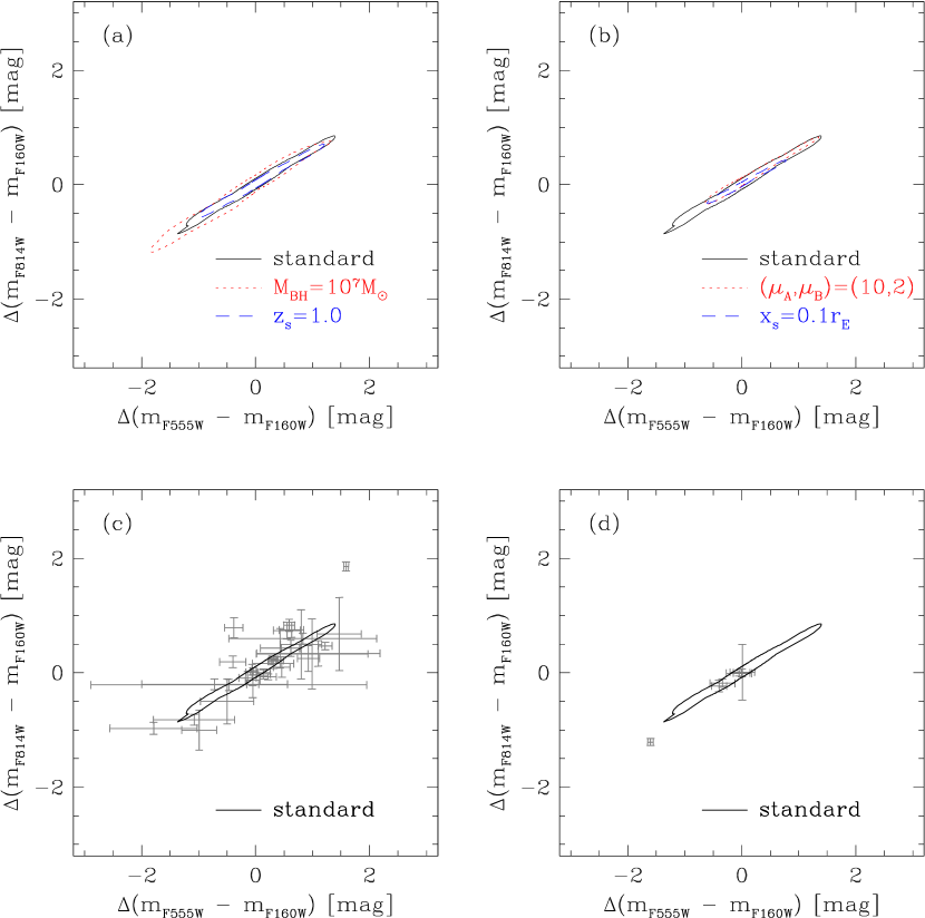
Figure 7: The expected color differences between multiple images due to quasar microlensing. The maximum color differences by quasar microlensing are presented by the lines. The upper two panels show the expected color difference for various parameter sets; $M_{\rm BH}$, $z_{s}$, $\mu_{A}$, $\mu_{B}$, and $x_{s}$. The solid line in all panel represents the expected color difference for $M_{\rm BH}=10^{8}M_{\odot}$, $z_{s}=2.0$, $(\mu_{A},\mu_{B})=(3.0,2.0)$, and $x_{s}=r_{E}$, and is referred to as ‘standard’ in all the panels. $M_{\rm lens}=1M_{\odot}$ and $z_{l}=0.5$ are applied for calculating $r_{E}$ in all the cases, and $r_{E}$ in this estimation is not on the lens plane, but on the source plane. In the upper left panel, panel (a), the expected color differences for $M_{\rm BH}=10^{7}M_{\odot}$ and for $z_{s}=1.0$ are presented by the dotted (red) and dashed (blue) lines, respectively. In the upper right panel, panel (b), the expected color difference for $(\mu_{A},\mu_{B})=(10,2)$ and for $x_{s}=0.1r_{E}$ are presented by the dotted (red) and the dashed (blue) line, respectively. The remaining parameters are the same as that for parameters of the ‘standard’ case. Observational data shown in Figure 2 (a) and (b) is plotted by gray crosses in panels (c) and (d), respectively, and the expected color differences for $M_{\rm BH}=10^{8}M_{\odot}$ presented in panel (a) are overlaid on these panels by the solid line.

It is apparent from Figure 7 that the maximum color difference depends strongly on $M_{\rm BH}$, $(\mu_{A},\mu_{B})$ and $x_{s}$, and weakly on $z_{s}$. Within a reasonable range for $z_{s}$ (e.g., see Figure 1), the rest frame wavelength which corresponds to the observational waveband varies by a factor of few. Thus, emissivity distributions for the observational wavebands at the different source redshift differs slightly. Not only due to the smaller source size, but also due to the bluer spectrum of the accretion, the expected color change for smaller $M_{\rm BH}$ shows different features than that for larger $M_{\rm BH}$, as shown by the dotted line in Figure 7 (a). For larger $\mu_{a}$, i.e., larger $\mu_{A}$, larger $\mu_{B}$ or both in these calculations, the color difference is suppressed as shown by the dotted line in Figure 7 (b). This can be understood from equations 9,  10 and 11. Magnitude changes due to quasar microlensing are determined by a ratio of a magnification for inside the caustics (equation 9) to a magnification for outside the caustics (equation 10) rather than a magnification for inside the caustics alone (see equation 11). Since the contribution of the term including $x$ in equation 9 to the magnitude change is relatively smaller in the larger $\mu_{a}$ case, the change due to microlensing becomes small, and consequently, the color change is smaller compared to the smaller $\mu_{a}$ case. This means that the magnification due to macrolensing could be crucial to quantify how much color difference would be expected from quasar microlensing. Of course, another major factor to estimate the color difference is a property of magnification pattern as shown with the dashed lines in Figure 7 (b). If we apply smaller $x_{s}$, only a part of the source is magnified by microlensing, and a smaller amount of color difference is expected (see equation 10).

Since the ‘standard’ parameter set in Figures 7 (a) and (b) can be a representative parameter set for actual quasar microlensing events, the expected color is also plotted with observational data in Figures 7 (c) and (d) for comparison. Quasar microlensing alone can also produce color differences up to $\sim 2{\rm\leavevmode\nobreak\ mag}$ which is similar to the scatter of observational data. Further, the observed color difference is well reproduced by quasar microlensing within the error bars except some individual data points, for instance the upper right data point in Figure 7 (c) and the lower left data point in in Figure 7 (d).

As is already noted in the case of quasar variabilities (section 3), the date of observations is different in different wavebands (e.g., Lehár et al., 2000), and we should take into account the interval among the multi-waveband observations for one object, $\Delta t$. However, conversion of the timescale of microlensing used in numerical calculation, e.g., see equation 8, into an actual timescale involves some ambiguities. Here, we applied $|\Delta t|\leq 50r_{s}/v_{c}$ and $|\Delta t|\leq 100r_{s}/v_{c}$ as the time difference with respect to the date of observation at F555W and calculate the expected color difference between images. That is, denoting the observational epoch at F555W in the microlensing light curve for two images by $t_{A}$ and $t_{B}$, the observational epoch for two images at F814W and F160W is $t_{A}+\Delta t$ and $t_{B}+\Delta t$, and $t_{A}+\Delta t^{\prime}$ and $t_{B}+\Delta t^{\prime}$, respectively, where $\Delta t$ and $\Delta t^{\prime}$ are uncorrelated and all possible combinations for $\Delta t$ and $\Delta t^{\prime}$ within the applied time difference are chosen for calculations. The maximum time difference of $|\Delta t|\leq 50r_{s}/v_{c}$ and $|\Delta t|\leq 100r_{s}/v_{c}$ corresponds to $\sim 1\leavevmode\nobreak\ {\rm yr}$ and $\sim 2\leavevmode\nobreak\ {\rm yr}$, respectively, in the case of $v_{c}=10^{3}\leavevmode\nobreak\ {\rm km\leavevmode\nobreak\ s^{-1}}$ and $M_{\rm BH}=10^{8}M_{\odot}$. The results are presented in Figure 8. As easily seen in Figure 8, the expected color difference with non-zero time difference among different wavebands (the dotted and the dashed lines in Figure 8a) is stretched toward an orthogonal direction to the major axis of the expected color difference calculated without time difference (the solid line in Figure 8a). An effect of time difference largely extends the theoretically allowed region of the expected color difference produced by quasar microlensing. Consequently, most of the observed color difference of multiple quasars including objects whose observed color difference cannot be reproduced by differential dust extinction are also nicely reproduced (Figure 8 (b)) .

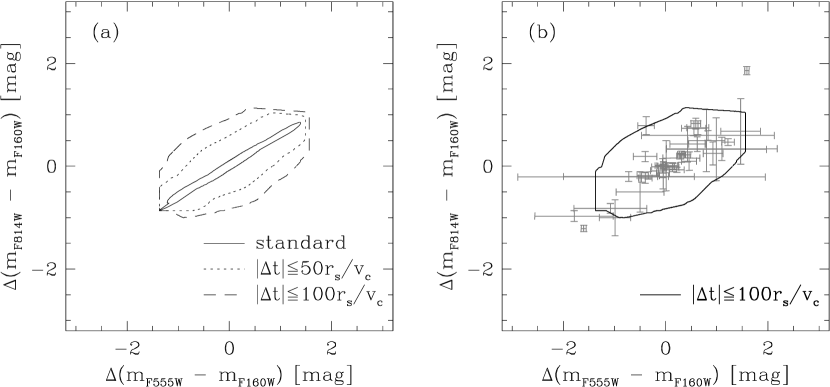
Figure 8: The expected color differences between multiple images due to quasar microlensing. Here, possible ranges of observations are included. ‘Standard’ set of parameters in Figure 7 are also applied for these calculations, and the result obtained without including the time difference, i.e., $|\Delta t|=0$, is presented as a reference by the solid line in the left panel, panel (a). In panel (a), the result for $|\Delta t|<50r_{s}/v_{c}$ and $|\Delta t|<100r_{s}/v_{c}$ is also presented by the dotted and the dashed line, respectively. Observational data shown in Figure 2 (a) and (b) are plotted by gray crosses in panels (b). The expected color difference in the case of $|\Delta t|<100r_{s}/v_{c}$ is also overlaid on this panel by the solid line.

Since we do not include any statistical properties of caustics such as distribution of the scale length of the caustics or clustering of the caustics the expected color differences can not reproduce distribution of the data points well . On one hand, therefore, we cannot directly compare to the results for quasar microlensing to the distribution of observational data (e.g., data points shown in Figure 8 (b)). The expected color differences presented here (e.g., a closed curve shown in Figure 8 (b)) are the maximum color differences which can be produced within the framework of our calculations with a given $x_{s}$.

On the other hand, the applied approximation for magnification due to quasar microlensing is surprisingly sufficient to reproduce the observed color differences. Our treatment, an approximation for magnification based on general properties of gravitational lensing, is rather simple compared to more realistic methods such as ray-shooting, and does not include any fine structure of the caustics such as curvature of fold caustics, cusp caustics , or an overlap of caustics. We suspect that our simple treatment is enough to reproduce the observed color differences since the observed color differences are mainly produced by isolated caustics and/or caustics with larger size compared to fine structures of caustics. Even if caustics with a typical size smaller than the source size overlap with caustics with a larger size, the former (smaller) caustics add only a tiny fluctuation of magnification, and cannot produce significant amount of color differences. Thus, we can interpret that our simple approach extract only the caustics which contribute to the strongest magnification at a certain moment. This putative explanation should be checked by more sophisticated calculations in future.

Even with quasar microlensing, it is clear that the observed color differences of some extreme objects which are located at a top-right corner and a bottom-left corner in Figure 8 (b) are not well reproduced. We will further discuss this issue in section 6.

6 Discussion

In this paper, we have examined the following three possibilities for explaining the observed chromaticity between multiple images of lensed quasars: (i) intrinsic variabilities of the lensed quasars, (ii) differential dust extinction in the lens galaxy, and (iii) quasar microlensing in the lens galaxy.

6.1 Overall trends

First, we have examined the intrinsic variabilities of the lensed quasars. Quasars generally have intrinsic variabilities, and there exists a time delay between multiple images of lensed quasars. Thus, the intrinsic variabilities of quasars could explain the observed color differences. However, we find that the expected value of the color difference is roughly one order of magnitude smaller than the observed color differences. Therefore, we can exclude the possibility that intrinsic variabilities are responsible for the observed color differences in the sample.

As shown in Figures 5 and 7, both differential dust extinction and quasar microlensing instead can reproduce the observed color differences. The color differences due to these two scenarios similarly reproduce the observational data points in Figures 5 and 7. However, once we take into account the time difference among the observations at different wavebands that usually happens in an actual situation, the area covered by the expected color difference of quasar microlensing expands, and we can reproduce the observed color difference by quasar microlensing alone, as shown in Figure 8. These results are also summarized in Figure 9; objects whose observed color differences are not reproduced by a single scenario alone, either differential dust extinction or quasar microlensing, are plotted with the expected color difference by our estimations. Although there is an ambiguity in converting a timescale used in our numerical calculations into an actual timescale, quasar microlensing proves to be a better scenario to reproduce observed color differences compared to other scenarios, if only one scenario is responsible for the observed color differences. In an actual situation, it is more probable that both effects play a role at the same time in producing the observed color differences. Combining these two scenarios (differential dust extinction and quasar microlensing), all the observed color differences presented in this paper seem to be nicely reproduced (see Figure 9); if we convolve the shaded region in Figures 9 (a) and (b), we may be able to reproduce the observed color differences (the gray crosses) shown in Figure 9 which cannot be reproduced by either differential dust extinction or quasar microlensing.

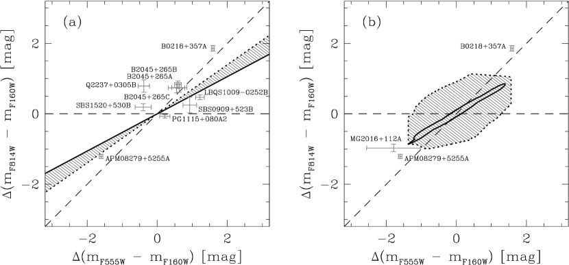
Figure 9: Objects whose observed color difference between multiple images is not well reproduced by our estimations are picked out and are presented with their name, and with the expected color difference by our estimations. In the left panel (panel a), the expected color difference for the MW extinction curve with $R_{V}=2.6$ and that for MW with $R_{V}=5.6$ are presented by the solid and dotted lines, respectively, where $z_{l}=0.5$ is assumed. The expected color difference locates between the solid and the dotted line, i.e., the shaded region. Objects whose observed color difference cannot be reproduced by differential dust extinction are also presented by the gray crosses. In the right panel (panel b), the expected color difference for ‘standard’ case of quasar microlensing and that including difference in observational epochs at different wavebands are presented by the solid and dotted lines, respectively, where $z_{s}=2.0$ is assumed. The expected color difference for ‘standard’ case with the non-zero spans locates inside the solid line, i.e., the shaded region. Again, objects whose observed color difference cannot be reproduced by quasar microlensing are presented by the gray crosses. The line for $\Delta m_{F814W}-\Delta m_{F160W}=0$ and the line for $\Delta m_{F555W}-\Delta m_{F160W}=\Delta m_{F814W}-\Delta m_{F160W}$ are also presented by the dashed lines as references.

Unfortunately, it is not possible to discriminate which one is dominating the observed color differences with only one photometric observation as used in this paper. Since differential extinction is a static phenomenon and quasar microlensing is a temporal phenomenon whose timescale is given by equations 7 and/or 8, multiple or monitoring observations of lensed quasars at multiple wavebands are the only way to distinguish between differential dust extinction and quasar microlensing. Multi-wavelength data taken at the same time or during negligibly short spans of observations compared to timescale of quasar microlensing are also required to suppress the color diversity caused by the time difference among the observations at different wavebands.

Of special interest are the properties of objects whose observed color differences are not reproduced by either differential dust extinction or quasar microlensing. Even if the observed color difference is within the expected color difference of our estimations, we have to care about quasar microlensing and/or intrinsic variabilities of quasars. Thus one should trace and separate effects of quasar microlensing and/or intrinsic quasar variabilities properly to derive the extinction curve of the lens galaxy: otherwise the extinction curves derived for lens galaxies may be contaminated by the microlensing and/or the intrinsic quasar variability effects, and it will be an unrealistic at the worst.

6.2 Peculiar features

Next, we focus on objects whose observed color differences are difficult to be reproduced by either differential dust extinction or quasar microlensing. In Figures 9 (a) and (b), we choose 8 objects (10 image pairs) whose color differences are not explained by differential dust extinction alone (B0218+357, SBS0909+523, LBQS1009-0252, PG1115+080, SBS1520+530, B2045+265, Q2237+0305, and APM08279+5255), and 3 objects (3 image pairs) whose color differences are not explained by quasar microlensing alone (B0218+357, MG2016+112, and APM08279+5255).

A possible explanation for eight objects deviating from the expected color difference in the differential dust extinction scenario is that the lens galaxies have a peculiar dust extinction which cannot be parameterized by the function that we have used in this paper. Since galaxies at different evolutionary stages are expected to have dust with different extinction properties (e.g., Maiolino et al., 2004; Hirashita et al., 2005), this would be one plausible explanation. Furthermore, Inoue et al. (2006) have shown that the wavelength dependence of the dust attenuation is modified by a effect of light scattering. An anomalous dust extinction (or attenuation) might be seen in a systematic difference in the colors of lens galaxies themselves. Thus, in order to check if the anomalous dust extinction is really responsible for the deviation from the model predictions, we examine the colors of the lens galaxies in Figure 10 (see also Table 2). Photometric data for the lens galaxies of B1600+434 and Q1208+101 are available not for all the bands, and the data are not plotted in Figure 10. B1030+071, MG2016+112, FBQ0951+2635, and Q0957+561 have another lens candidate, and the data are also plotted in Figure 10.

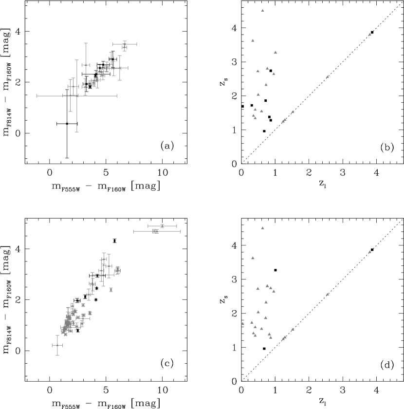
Figure 10: Relations between the quantities concerning the lens galaxies and the source quasars. The black filled squares in the upper and lower panels represent the objects that have deviation from the expected color difference by differential dust extinction and by quasar microlensing, respectively. Properties for the remaining objects are also plotted by the gray filled triangles. The color-color diagram for the lens galaxies and the source quasars are presented in panels (a) and (c), respectively. In panels (b) and (d), the lens redshift and the source redshift are presented in the same way as panels (a) and (c). The objects with unknown lens redshifts are plotted on the diagonal dotted line.

Unfortunately, as we can see in Figure 10(a), this explanation does not seem to be confirmed. Colors of the lens galaxy of objects with the unexpected color differences and that with the expected color differences are compared in Figure 10(a). The average color for the former objects are $(m_{F555W}-m_{F160W},m_{F814W}-m_{F160W})=(3.93\pm 1.12,2.11\pm 0.74)$, and that for the latter objects are $(m_{F555W}-m_{F160W},m_{F814W}-m_{F160W})=(4.35\pm 1.40,2.33\pm 0.53)$. The average color of the lens galaxy of objects with the unexpected color differences is slightly bluer than the others, but these values are overlapping each other within the dispersion. Thus, we can say that these two groups are not separated clearly as far as the galaxy color is concerned. Further, there is no clear difference between the redshifts of these two groups. The average redshifts are $(z_{l},z_{s})=(0.62\pm 0.30,1.94\pm 0.88)$ and $(z_{l},z_{s})=(0.61\pm 0.23,2.36\pm 0.97)$ for the objects with the unexpected color differences and the others, respectively (see also Figure 10 b).

In principle, dust extinction should be larger at shorter wavelength. This limit corresponds to the dashed lines in Figure 9; the horizontal line indicates that absorption at $F814W$ and that at $F160W$ is equal, and the diagonal line shows that absorption at $F555W$ and that at $F814W$ are equal. Therefore, the color differences by dust extinction should always be between the dashed lines in Figure 9(a). In other words, the color difference of objects that are not located in this region is not reproduced by dust extinction alone. As shown in Table 2, some of the lens galaxies are known to have observational properties of late-type galaxies; B0218+357, RXJ0911+0551, B1030+071, SBS1520+530, B1600+434, B2045+265, and MG2016+112, and dust properties in such systems may be somehow different from that in the MW or the SMC. It is still possible to explain the color differences in B2045+265 by differential extinction of dust with special properties because the color differences are located at “allowed” area for differential dust extinction. However, color differences in B0218+357, SBS1520+530, and Q2237+0305 are located at “prohibited” area for differential dust extinction, and their anomalous color differences are hard to be explained by differential dust extinction alone, if dust extinction is assumed to cause reddening in any wavelength. However, as can be seen from Figure 10, there is no clear evidence for peculiarity in the colors and redshifts of the objects whose deviation from the models is large with respect to other objects.

As for the 3 objects deviated from the expected color difference in the quasar microlensing scenario, it is possible that the lensed quasar have a peculiar physical properties of an accretion disk which cannot be well represented by the standard accretion disk model that we have used in this paper. Since the expected color differences by quasar microlensing may depend on the radiative properties of the central engine of quasars, a systematic difference in the source color between these two groups would be expected. In Figure 10(c), we present the color-color diagram of all the source quasar images. Again, however, no clear difference between these two groups is found. The average colors of the source quasars of the systems with unexpected and expected color differences from our microlensing models are $(m_{F555W}-m_{F160W},m_{F814W}-m_{F160W})=(3.76\pm 1.08,2.37\pm 1.00)$ and $(m_{F555W}-m_{F160W},m_{F814W}-m_{F160W})=(3.03\pm 2.31,1.75\pm 1.16)$, respectively. Thus, as long as we focus on the colors of the source quasars, we cannot find any significant difference between these two groups. Further, there is no clear difference between the redshifts of these two groups. The average redshifts are $(z_{l},z_{s})=(0.85\pm 0.17,2.70\pm 1.25)$ and $(z_{l},z_{s})=(0.58\pm 0.24,2.16\pm 0.90)$ for the objects with the unexpected color differences and the others, respectively (see also Figure 10 d).

A part of objects whose observed color differences are difficult to reproduce has been observed with more wavebands than others. For instance, B0218+357 and APM08279+5255 have been observed with 6 and 5 different wavebands, respectively. By using those data, we can examine the color differences between images more intensively. In Figure 11, we present the magnitude differences between images. In the case of APM08279+5255, the trend is rather simple. The magnitude difference monotonically decreases with increasing wavelength, and bluer photons are absorbed more than redder photons at image B and/or are magnified more than redder photons at image A. As we can also see from Figure 9, the color difference can be reproduced by a flatter extinction law and/or a larger scale length of caustics than that we used in this paper. The extinction law becomes flatter if the grain size distribution is more biased to a larger size. Furthermore, a larger scale length of caustics is also realized by taking into account large variety of caustics (e.g., Appendix C), and thus, it is possible to reproduce observed color differences of APM08279+5255 either by dust extinction or by quasar microlensing. However, the trend is complicated in the case of B0218+357, because the observed color difference seems to have a peak around $7000\AA$. If we can treat two data sets presented in Figure 11 equivalently, the magnitude difference is 0.5–1.0 mag at $\sim 3000\AA$ and at $\sim 16000\AA$, but is $\sim 2.5{\rm mag}$ at $\sim 7000\AA$. It is clear that the magnitude difference rapidly increases up to a wavelength of $\sim 5000\AA$ and becomes almost constant at wavelengths of $\sim 5000--8000\AA$. Such a wavelength dependence cannot be reproduced by dust grains. In contrast, quasar microlensing can magnify a part of quasar accretion disk selectively, and an emitting region of photons with a wavelength of $\sim 7000\AA$ can be selectively magnified with a certain configuration of the accretion disk and caustics. Further, if photons with wavelength above $\sim 7000\AA$ mainly originate from more extended region than the accretion disk, such as a lobe of jets, a torus or a starburst region, these photons cannot strongly be magnified by microlensing. Considering this possibility of microlensing, B0218+357 is more likely to be magnified by quasar microlensing than dust extinction.

Figure 11: Magnitude difference at several wavebands between images of B0218+357 (upper panel) and APM08279+5255 (lower panel). These data are also provided by CASTLES web page. For B0218+357, magnitude differences (magnitude of image A minus that of image B, the brightest image at F160W of HST NICMOS) at F300W, F380W, F439W, F555W, F675W, and F814W of HST WFPC2 are presented by the solid error bars. Data used previously in this paper are different sequence from these photometric data at 6 wavebands, and the data used previously are also presented by the dashed error bars as references. For APM08279+5255, magnitude differences at F555W and F814W of HST WFPC2, and at F110W, F160W, and F205W of HST NICMOS are presented. The solid error bars indicate that magnitude of image B minus that of image A, the brightest image at F160W.

As for the observational properties of objects whose observed color differences are not reproduced by either differential dust extinction or quasar microlensing, we cannot find any clear difference between these objects and the objects whose observed color differences are well reproduced by either differential dust extinction or quasar microlensing. Therefore, the peculiarity of lens galaxies or lensed quasars is unlikely to be a probable reason for the extreme color differences. It may be more natural to consider that all the observed color differences can be reproduced by a combination of all three possibilities presented in this paper without requiring any special properties of dust and/or quasar.

6.3 Concluding remarks

It is worth mentioning that there are some limitations in our current treatments of differential dust extinction and quasar microlensing.

For differential dust extinction, we have applied empirical extinction laws derived for the local universe such as the MW and the SMC. Although the observational color differences are roughly consistent with the local extinction curves, the extinction laws in distant galaxies such as the lens galaxies may be significantly different from the local ones, especially in lens galaxies whose data points deviate significantly from our calculations in Figure 5. In contrast, we have used gas distribution obtained by a numerical simulation for a disk galaxy (see Hirashita et al., 2003) to investigate the expected differential dust extinction. The current sample of lens galaxies involves both early- and late-type galaxies (see Table 2), which may have very different gas and dust properties. To take into account such variety of lens galaxies, gas and dust distribution for various types of galaxies, especially for early-type galaxies, and further exploration by using the distribution is required.

For quasar microlensing, we applied a straight line caustic approximation and did not take into account complex caustic networks (e.g., Wambsganss & Paczyński, 1991; Goicoechea, et al., 2005) that would be expected in most of systems. On the one hand, multiple caustics will produce more dramatic and/or complex structures in the expected light curves of quasar microlensing, and even larger or more strange features will be expected in the observed color difference. On the other hand, caustics with short scale length, i.e., small $x_{s}$, or small caustics can just slightly change the observed color during microlensing events. As already pointed out by Yonehara et al. (1998), the expected color difference also depends on accretion disk models for quasars, because the spatial emissivity distribution and the wavelength dependence is diverse in different accretion disk models such as a radiatively inefficient accretion flow. For instance, as presented in Yonehara et al. (1998), the expected light curves of microlensing of an advection-dominated accretion flow (ADAF) is almost achromatic, at least in optical wavebands, since the spatial emissivity distribution of ADAF is almost independent of the wavelength. Thus, the ADAF model has difficulty in explaining the achromaticity of lensed quasars. Though the dependence on the source emissivity profile is less prominent in statistical properties of the light curves (Mortonson et al., 2005), there exists clear dependence not only on the source size but also on the source emissivity profile in individual light curves. Quantitative estimates of various complexity caused by a variety of extinction curve, of caustic networks, and of accretion disks are addressed in future works.

Appendix A Extinction Law in the SMC

Gordon et al. (2003) have investigated extinction curves of the Small Magellanic Cloud (SMC), the Large Magellanic Cloud, and the Milky Way by using photometric data in the wavelength range from ultraviolet to near-infrared. Since the coefficient $C_{1}$ in equation (5) of Gordon et al. (2003) is negative Table 3 in Gordon et al., 2003 for the SMC, the extinction at some long wavelength becomes negative value, i.e., $A(x\rightarrow 0)<0$ for positive $A_{V}$. This may not be ideal in some situation, and we made a fitting formulae for it by ourselves by using the same data for the SMC denoted “SMC Bar” in Table 4 of Gordon et al., 2003.

We have adopted the same functional form of the extinction curve as the one provided by equation 1 in Cardelli et al. (1989) in our fitting procedures. We apply the same function form as $a(x)$ in Cardelli et al. (1989), and the fit is satisfactory as shown later. The number of parameters to be determined is 20 in total; 1 coefficient and 1 power index at $\lambda^{-1}\leq 1.1\leavevmode\nobreak\ {\rm\mu m^{-1}}$, 7 coefficients at $1.1\leavevmode\nobreak\ {\rm\mu m^{-1}}\leq\lambda^{-1}\leq 3.3\leavevmode\nobreak\ {\rm\mu m^{-1}}$, 7 coefficients at $3.3\leavevmode\nobreak\ {\rm\mu m^{-1}}\leq\lambda^{-1}\leq 8.0\leavevmode\nobreak\ {\rm\mu m^{-1}}$, and 4 coefficients at $8.0\leavevmode\nobreak\ {\rm\mu m^{-1}}\leq\lambda^{-1}$. We have determined those coefficients by performing $\chi^{2}$ minimization with a downhill simplex method (Press et al., 1992).

The resultant formulae for the extinction as a function of the inverse of wavelength ($x=\lambda^{-1}$ in $\mu$m^-1) is as follows;

$$\frac{A(x)}{A_{V}} = 0.31884x^{3.57967}\leavevmode\nobreak\ \leavevmode\nobreak\ \leavevmode\nobreak\ (x\leq 1.1)$$

$$= 1+0.92733p-0.31777p^{2}-0.83093p^{3}+1.58876p^{4}$$

$$+0.60622p^{5}-1.91599p^{6}+0.71769p^{7}\leavevmode\nobreak\ \leavevmode\nobreak\ \leavevmode\nobreak\ (1.1\leq x\leq 3.3)$$

$$= -0.77359+0.81739x+\frac{0.02248}{\left(x-4.54152\right)^{2}+0.13635}$$

$$+0.23260q^{2}-0.06653q^{3}\leavevmode\nobreak\ \leavevmode\nobreak\ \leavevmode\nobreak\ (3.3\leq x\leq 8.0)$$ (15)

$$= 6.17700+2.39744r-8.90103r^{2}+11.44564r^{3}\leavevmode\nobreak\ \leavevmode\nobreak\ \leavevmode\nobreak\ (8.0\leq x),$$ (16)

where $p=x-1.82$, $q=x-5.9$, and $r=x-8.0$. The $\chi^{2}$ value for the best fit parameters is $36.28$. Since the number of data points that we have used in our fitting is 30 and the degree of freedom becomes $30-20=10$, the reduced $\chi^{2}$ value clearly exceeds $1.0$ and thus is not particularly good. This mainly originates in a few data points with small error bars at longer wavelength, and we can see in Figure 12 that our fitting result nicely traces most of the data points, especially in the wavelength range relevant in this paper.

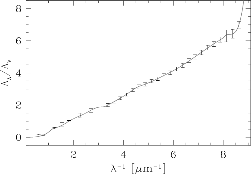
Figure 12: The SMC extinction curve obtained by our fitting procedure is shown by the gray solid line. Abscissa is inverse of wavelength ($\lambda^{-1}$), and ordinate is extinction value divided by extinction at $V$ band ($A_{\lambda}/A_{V}$). Data points with the error used in our fitting procedure originally presented by Gordon et al., 2003 are overlaid as the black bars on the extinction curve.

Appendix B Supplementary remarks for individual objects

B.1 Possible evidence for quasar microlensing

From previous measurements, the existence of a quasar microlensing signal is quite obvious from their observed light curves. For instance, Q2237+0305 has frequently shown clear microlensing signals (e.g., Woźniak et al., 2000) in the photometric data since the first detection of microlensing by Irwin et al. (1989). Additionally, due to the large leverage arm of the nearby lens galaxy, the transverse velocity of the caustics on the source plane is enhanced by a factor of $10$ from that of other lensed quasars, and the typical timescale of the microlensing events is reduced by the same factor.

Possible microlensing signals in optical wavebands are suggested in Q0957+561 by Colley & Schild (2000); Goicoechea, et al. (2005), and ones in radio wavebands are suggested in B1600+434 by Koopmans et al. (2001). Burud et al. (2000) have also shown a possibility of quasar microlensing signal in the $I$-band monitoring data of B1600+434.

For the measurement of time delay between images, contributions from quasar microlensing are included in the analysis, and the goodness of fit is improved substantially by including effects of quasar microlensing. From this point of view, the existence of quasar microlensing is indicated indirectly in a subset of the current sample, PG1115+080 (Barkana, 1997), RXJ0911+0551 (Hjorth et al., 2002), HE1104-1805 (Ofek & Maoz, 2003), SBS1520+530 (Gaynullina, et al., 2005), and FBQ0951+2635 (Jakobsson et al., 2005). Observations of all these objects are performed at optical wavebands.

For LBQS1009-0252, sparse multi-color monitoring observations have been done and some spectra have been obtained by (Claeskens et al., 2001). Claeskens et al. (2001) have focused on the changes of colors and spectra during the observations and have mentioned a possible existence of dust extinction and/or microlensing in this system. However, it may be possible to explain the changes by intrinsic variabilities.

In the case of Q0142-100, evidence for quasar microlensing is considered to be obtained from the observed color changes in optical monitoring data (Nakos et al., 2005).

Also in the case of HE2149-2745, quasar microlensing is suggested to explain unexpected spectral differences between images (Burud et al., 2002a).

B.2 Other remarks

One of the most famous lensed quasars, Q0957+561, is in a somewhat special environment compared to other objects, because the lens galaxy is obviously a member of a galaxy cluster (e.g., Angonin-Willaime et al., 1994).

MG2016+112 is supposed to have two lens galaxies. Although the lens galaxies show the brightness profile of early type galaxies, one or both of the lens galaxies show an [O ii] emission line (Koopmans & Treu, 2002).

Radio monitoring observations of MG0414+0534 have been performed by Moore & Hewitt (1997). Unfortunately, the intrinsic flux variation of this quasar seems to be small, and a time delay measurement has not been successful.

B1030+074 has been detected by Xanthopoulos et al. (1998), and at the same time, they claimed that an image of the lens galaxy which is taken by HST shows substructure which could be a spiral arm or an interacting galaxy.

For B2045+265, all the three images show almost the same color difference from, or redder than, the brightest image in F160W filter (see Figure 9). However, it is not probable that three of four images are occasionally affected by dust extinction and/or quasar microlensing in the same way. Rather, it would be reasonable to consider that only the brightest image in F160W filter is predominantly affected by dust extinction and/or quasar microlensing, which cause a common color difference for the remaining three images.

Appendix C Scale Length of Caustics

To estimate color changes produced by quasar microlensing, we have applied a simple approximation in the vicinity of fold caustics shown in equation 9. This approximation formula includes a scale length which is denoted by $x_{s}$, and this scale length is not arbitral but determined by a property of the caustics (e.g., Schneider et al., 1992), i.e., external convergence and shear, and distribution of lens objects. Here, we briefly investigate how to estimate the length, and we present the expected value.

C.1 Definition of the scale length

By using a lens potential, $\psi$, the lens equation for quasar microlensing with $N$ point mass lenses is expressed as

$$0 = \frac{\partial\psi}{\partial\theta_{x}}\equiv-\beta_{x}+(1-\kappa_{c})\theta_{x}+\gamma(\cos 2\phi\theta_{x}+\sin 2\phi\theta_{y})-\sum_{i=1}^{N}\left(\frac{\alpha^{[i]}}{\left|{\bf\theta}-{\bf\theta^{[i]}}\right|}\right)^{2}(\theta_{x}-\theta_{x}^{[i]})$$ (17)

$$0 = \frac{\partial\psi}{\partial\theta_{y}}\equiv-\beta_{y}+(1-\kappa_{c})\theta_{y}+\gamma(\sin 2\phi\theta_{x}-\cos 2\phi\theta_{y})-\sum_{i=1}^{N}\left(\frac{\alpha^{[i]}}{\left|{\bf\theta}-{\bf\theta^{[i]}}\right|}\right)^{2}(\theta_{y}-\theta_{y}^{[i]}),$$ (18)

where $\beta_{x}$, $\beta_{y}$, $\theta_{x}$, $\theta_{y}$, $\theta_{x}^{[i]}$, $\theta_{y}^{[i]}$, $\alpha^{[i]}$, $\kappa_{c}$, $\gamma$, and $\phi$ represent $x-$ and $y-$ coordinates of source, $x-$ and $y-$ coordinates of image (${\bf\theta}$), $x-$ and $y-$ coordinates of $i-$th lens (${\bf\theta^{[i]}}$), Einstein ring radius of $i-$th lens, convergence due to smooth matter, external shear and direction of the shear, respectively. For a practical convenience in deriving the approximation formula, the coordinate systems are chosen such that the origin of the lens plane and the source plane is located on critical curves and caustics, respectively, and $y-$axis of the source plane is orthogonal to the fold caustics. Performing the Taylor expansion and applying conditions in the vicinity of the fold caustics, we can obtain the following expression for magnification ($\mu$) after some algebra,

$$\mu(\beta_{x},\beta_{y})\simeq\left[\frac{1}{2}\left(\left.\frac{\partial^{2}\psi}{\partial\theta_{x}^{2}}\right|_{(0,0)}\right)^{2}\left.\frac{\partial^{3}\psi}{\partial\theta_{y}^{3}}\right|_{(0,0)}\beta_{y}\right]^{-1/2}.$$ (19)

Here, the caustics are assumed to be straight lines, and the dependence on $\beta_{x}$ disappears from the magnification. This is the same form as the first term in equation 9 for inside the caustics, and now it is clear that the scale length in equation 9 should be

$$x_{s}=2\left[\left(\left.\frac{\partial^{2}\psi}{\partial\theta_{x}^{2}}\right|_{(0,0)}\right)^{2}\left.\frac{\partial^{3}\psi}{\partial\theta_{y}^{3}}\right|_{(0,0)}\right]^{-1}.$$ (20)

See Schneider et al. (1992) for more details.

C.2 Efficient method to estimate the scale length

Although the magnification probability of quasar microlensing depends on the mass spectrum of the lens objects (Schechter et al., 2004), we assumed that all the lenses have the same mass. Further, all the length scales ($x_{s}$) are normalized to the Einstein ring radius for an assigned lens mass, and $\alpha^{[i]}$ is set to be unity here. The following estimation method can be applicable also if the mass spectrum is taken into account.

In addition to equations 17 and 18, the following conditions should also be satisfied on fold caustics, or corresponding critical curves, i.e., at $(\theta_{x},\theta_{y})=(0,0)$;

$$0 = \frac{\partial^{2}\psi}{\partial x\partial y}\equiv\gamma\sin 2\phi+\sum_{i=1}^{N}\frac{2(\theta_{x}-\theta_{x}^{[i]})(\theta_{y}-\theta_{y}^{[i]})}{\left|{\bf\theta}-{\bf\theta}^{[i]}\right|^{4}}$$ (21)

$$0 = \frac{\partial^{2}\psi}{\partial y^{2}}\equiv(1-\kappa_{c})-\gamma\cos 2\phi+\sum_{i=1}^{N}\frac{(\theta_{y}-\theta_{y}^{[i]})^{2}-(\theta_{x}-\theta_{x}^{[i]})^{2}}{\left|{\bf\theta}-{\bf\theta}^{[i]}\right|^{4}}$$ (22)

$$0 \neq \frac{\partial^{2}\psi}{\partial x^{2}}\equiv(1-\kappa_{c})+\gamma\cos 2\phi+\sum_{i=1}^{N}\frac{(\theta_{x}-\theta_{x}^{[i]})^{2}-(\theta_{y}-\theta_{y}^{[i]})^{2}}{\left|{\bf\theta}-{\bf\theta}^{[i]}\right|^{4}}$$ (23)

$$0 \neq \frac{\partial^{3}\psi}{\partial y^{3}}\equiv\sum_{i=1}^{N}2(\theta_{y}-\theta_{y}^{[i]})\frac{3(\theta_{x}-\theta_{x}^{[i]})^{2}-(\theta_{y}-\theta_{y}^{[i]})^{2}}{\left|{\bf\theta}-{\bf\theta}^{[i]}\right|^{6}}.$$ (24)

As we can recognize in the above equations, equation 23 is simply reduced to $2(1-\kappa_{c})$ by using equation 22. Therefore, the only term we should evaluate to estimate $x_{s}$ is the third derivative expressed in equation 24. A condition for equation 24 corresponds to a condition to avoid cusp caustics.

Since the above equations should be satisfied on fold caustics or corresponding critical curves, i.e., $(\theta_{x},\theta_{y})=(0,0)$, equations 17, 18, 21, and 22 can be rewritten as the following forms,

$$0 = \sum_{i=1}^{N-2}\frac{\theta_{x}^{[i]}}{\left|{\bf\theta^{[i]}}\right|^{2}}+\frac{\theta_{x}^{[N-1]}}{\left|{\bf\theta^{[N-1]}}\right|^{2}}+\frac{\theta_{x}^{[N]}}{\left|{\bf\theta^{[N]}}\right|^{2}}$$ (25)

$$0 = \sum_{i=1}^{N-2}\frac{\theta_{y}^{[i]}}{\left|{\bf\theta}^{[i]}\right|^{2}}+\frac{\theta_{y}^{[N-1]}}{\left|{\bf\theta}^{[N-1]}\right|^{2}}+\frac{\theta_{y}^{[N]}}{\left|{\bf\theta}^{[N]}\right|^{2}}$$ (26)

$$0 = \gamma\sin 2\phi+\sum_{i=1}^{N-2}\frac{2\theta_{x}^{[i]}\theta_{y}^{[i]}}{\left|{\bf\theta}^{[i]}\right|^{4}}+\frac{2\theta_{x}^{[N-1]}\theta_{y}^{[N-1]}}{\left|{\bf\theta}^{[N-1]}\right|^{4}}+\frac{2\theta_{x}^{[N]}\theta_{y}^{[N]}}{\left|{\bf\theta}^{[N]}\right|^{4}}$$ (27)

$$0 = (1-\kappa_{c})-\gamma\cos 2\phi+\sum_{i=1}^{N-2}\frac{(\theta_{y}^{[i]})^{2}-(\theta_{x}^{[i]})^{2}}{\left|{\bf\theta}^{[i]}\right|^{4}}+\frac{(\theta_{y}^{[N-1]})^{2}-(\theta_{x}^{[N-1]})^{2}}{\left|{\bf\theta}^{[N-1]}\right|^{4}}+\frac{(\theta_{y}^{[N]})^{2}-(\theta_{x}^{[N]})^{2}}{\left|{\bf\theta}^{[N]}\right|^{4}}.$$ (28)

Distributing the lens objects with the index from $i=1$ to $i=N-2$ randomly, equations 25, 26, 27, and 28 are equivalent with 4 equations for 4 unknown quantities ($\theta_{x}^{[N-1]}$, $\theta_{y}^{[N-1]}$, $\theta_{x}^{[N]}$, and $\theta_{y}^{[N]}$) for given $\gamma$ and $\phi$. By solving those 4 equations, we can obtain locations of two lens objects to create fold caustics on the origin of the applied coordinate. Substituting locations of all the lens objects including ${\bf\theta}^{[N-1]}$ and ${\bf\theta}^{[N]}$ into equation 24, we can obtain $x_{s}$ for the fold caustics in this realization of distribution of the lens objects. If the number of the lens objects which are randomly distributed on the lens plane ($N-2$ in this case) is large enough compared to the number of the lens objects which are added to create the fold caustics at a certain place on the source plane ($2$ in this case), the resultant distribution of the lens objects can be also treated as a random distribution.

An advantage of this procedure is that calculations of caustics networks are not required, and that computations for one realization are very fast. Although the procedure can only provide $x_{s}$ of caustics rather than the whole magnification pattern, it is efficient to investigate statistical properties of $x_{s}$. The procedure must be useful to evaluate a proper value of $x_{s}$ for a given environment, i.e., total convergence ($\kappa$), $\kappa_{c}$, and $\gamma$.

We have estimated $x_{s}$ with $10^{4}$ lens objects (i.e., $N=10^{4}$) for several values of $\kappa$, $\kappa_{c}$, and $\gamma$. All the lens objects except the last two, $(N-1)-$th and $N-$th lens objects, are randomly distributed within a circle. Radius of the circle is determined so that the surface density of the lens objects is equal to $\kappa-\kappa_{c}$, i.e., $\left[N/(\kappa-\kappa_{c})\right]^{1/2}$. Direction of external shear, $\phi$, is also chosen randomly at every realization. We have performed $10^{5}$ realizations to obtain the expected distributions of $x_{s}$, and results are presented in Figure 13.

Figure 13: Cumulative probability distributions of the scale length of fold caustics, $x_{s}$. Abscissa is $x_{s}$ in units of the Einstein ring radius ($r_{E}$). In the top panel (panel a), total convergence ($\kappa$) and external shear ($\gamma$) are fixed to $0.5$. Distributions for a fraction of smooth matter ($\kappa_{c}/\kappa$) equals $0.0$, $0.5$, and $0.9$ are presented by the dashed, solid, and dotted lines, respectively. In the middle panel (panel b), $\kappa_{c}/\kappa$ and $\gamma$ are fixed as $0.5$. Distributions for $\kappa=0.8$, $0.5$, and $0.2$ are presented by the dashed, solid, and dotted line, respectively. In the bottom panel (panel c), $\kappa$ and $\kappa_{c}/\kappa$ are fixed as $0.5$. Distributions for $\gamma=0.8$, $0.5$, and $0.2$ are presented by the dashed, solid, and dotted line, respectively.

First, the distribution depends on the fraction of smooth matter with respect to the total convergence, $\kappa_{c}/\kappa$. The scale length $x_{s}$ becomes smaller as $\kappa_{c}/\kappa$ becomes smaller. Since $\kappa_{c}/\kappa$ cannot be smaller than $0$, the dashed line in Figure 13(a) can be treated as a minimum of $x_{s}$ distribution for given $\kappa$ and $\gamma$. Although it is practically difficult to investigate $\kappa_{c}/\kappa$, we obtain the minimum of $x_{s}$ for $\kappa=0.5$ and $\gamma=0.5$ as $\sim 10^{-3}$ from Figure 13(a) . Second, as is shown in Figure 13(b) and (c), dependence on $\kappa$ and $\gamma$ is weak. The minimum value of $x_{s}$ increases slightly with decreasing $\kappa$, and the maximum value of $x_{s}$ increases slightly with decreasing $\gamma$. Especially, the dependence of the $x_{s}$ distribution on $\gamma$ is almost negligible. Although the distribution of $x_{s}$ shows a slight dependence on $\kappa_{c}/\kappa$, $\kappa$, and $\gamma$, we can conclude that typical value of $x_{s}$ is within a range of 0.1 – 1 as shown in Figure 13. Several scale lengths at certain cumulative probabilities are also summarized in Table 4 for convenience.

Table 4: The scale lengths of caustics, $x_{s}$, at certain cumulative probabilities for distributions presented in Figure 13 are listed. The column for $50\%$ indicates the median value of the distributions. $15.85\%$ and $84.15\%$ indicate the $\pm 1\sigma$ confidence levels from the median value, and $0.135\%$ and $99.865\%$ indicate the $\pm 3\sigma$ confidence levels from the median value.

$\kappa$	$\kappa_{c}/\kappa$	$\gamma$	$0.135\%$	$15.85\%$	$50\%$	$84.15\%$	$99.865\%$
0.5	0.5	0.5	$9.86\times 10^{-5}$	$5.79\times 10^{-2}$	$2.83\times 10^{-1}$	$1.33$	$1.61\times 10^{2}$
0.5	0.9	0.5	$2.04\times 10^{-3}$	$7.51\times 10^{-1}$	$2.20$	$9.23$	$1.29\times 10^{3}$
0.5	0.0	0.5	$1.96\times 10^{-5}$	$1.18\times 10^{-2}$	$6.37\times 10^{-2}$	$3.42\times 10^{-1}$	$4.80\times 10^{1}$
0.2	0.5	0.5	$2.70\times 10^{-4}$	$1.21\times 10^{-1}$	$4.18\times 10^{-1}$	$1.57$	$1.65\times 10^{2}$
0.8	0.5	0.5	$7.62\times 10^{-5}$	$4.63\times 10^{-2}$	$2.53\times 10^{-1}$	$1.38$	$1.82\times 10^{2}$
0.5	0.5	0.2	$9.86\times 10^{-5}$	$5.84\times 10^{-2}$	$2.98\times 10^{-1}$	$1.52$	$2.06\times 10^{2}$
0.5	0.5	0.8	$9.85\times 10^{-5}$	$5.66\times 10^{-2}$	$2.59\times 10^{-1}$	$1.15$	$1.44\times 10^{2}$

Table 2: Current sample of lensed quasars. The redshifts of the lens galaxy ($z_{l}$) and of the source quasar ($z_{s}$), the colors of the lensed quasar images and the errors for F555W - F160W ($m_{F555W}-m_{F160W}$), and for F814W - F160W ($m_{F814W}-m_{F160W}$) are presented. These colors should be identical for each image of the same lensed quasar unless intrinsic variability, dust extinction, or microlensing play a significant role. The magnitudes of the images at F160W ($m_{F160W}$) are also presented in the last column. The redshifts of the lens galaxies are not known for the 6 objects listed at the bottom. All the data are taken from the CASTLES web page, and the colors are calculated from these data.

Object Name	$z_{l}$	$z_{s}$	$m_{F555W}-m_{F160W}$	$m_{F814W}-m_{F160W}$	$m_{F160W}$
Q0142-104 A	0.49	2.72	$1.61\pm 0.092$	$1.34\pm 0.181$	$15.28\pm 0.02$
B			$1.56\pm 0.050$	$1.14\pm 0.153$	$17.57\pm 0.03$
B0218+357 A	0.68	0.96	$5.76\pm 0.036$	$4.31\pm 0.073$	$17.52\pm 0.02$
B			$4.17\pm 0.022$	$2.45\pm 0.028$	$16.94\pm 0.02$
MG0414+0534 A1	0.96	2.64	$9.99\pm 1.270$	$4.89\pm 0.063$	$15.54\pm 0.02$
A2			$10.82\pm 0.272$	$5.49\pm 0.067$	$15.87\pm 0.03$
B			$9.52\pm 2.080$	$4.68\pm 0.076$	$16.56\pm 0.03$
C			$9.27\pm 0.141$	$4.69\pm 0.073$	$17.41\pm 0.02$
B0712+472 A	0.41	1.34	$3.78\pm 0.277$	$2.64\pm 0.434$	$20.46\pm 0.21$
B			$4.58\pm 0.231$	$3.14\pm 0.422$	$21.08\pm 0.22$
C			$5.25\pm 0.272$	$3.32\pm 0.467$	$21.05\pm 0.08$
D			$4.77\pm 0.940$	$2.97\pm 0.433$	$21.90\pm 0.14$
RXJ0911+0551 A	0.77	2.80	$1.24\pm 0.045$	$0.79\pm 0.045$	$17.59\pm 0.02$
B			$1.53\pm 0.054$	$0.99\pm 0.036$	$17.65\pm 0.02$
C			$1.55\pm 0.067$	$1.02\pm 0.050$	$18.34\pm 0.03$
D			$1.62\pm 0.102$	$1.01\pm 0.036$	$18.65\pm 0.02$
SBS0909+523 A	0.83	1.38	$2.53\pm 0.082$	$1.95\pm 0.028$	$14.60\pm 0.02$
B			$3.46\pm 0.173$	$2.20\pm 0.222$	$14.73\pm 0.03$
BRI0952-0115 A	0.63	4.50	$3.59\pm 0.036$	$1.46\pm 0.045$	$17.07\pm 0.02$
B			$3.55\pm 0.036$	$1.49\pm 0.045$	$18.44\pm 0.02$
Q0957+561 A	0.36	1.41	$1.49\pm 0.085$	$1.11\pm 0.104$	$15.60\pm 0.03$
B			$1.43\pm 0.067$	$1.10\pm 0.095$	$15.68\pm 0.03$
LBQS1009-0252 A	0.87	2.74	$1.75\pm 0.082$	$1.32\pm 0.036$	$16.63\pm 0.02$
B			$2.97\pm 0.089$	$1.79\pm 0.057$	$18.20\pm 0.04$
B1030+071 A	0.60	1.54	$4.82\pm 0.221$	$3.59\pm 0.250$	$15.88\pm 0.02$
B			$3.83\pm 0.212$	$2.59\pm 0.242$	$19.79\pm 0.03$
HE1104-1805 A	0.73	2.32	$1.35\pm 0.321$	$0.81\pm 0.050$	$15.57\pm 0.03$
B			$1.66\pm 0.165$	$0.97\pm 0.064$	$17.04\pm 0.04$
PG1115+080 A1	0.31	1.72	$1.19\pm 0.112$	$0.71\pm 0.028$	$15.71\pm 0.02$
A2			$1.41\pm 0.095$	$0.64\pm 0.042$	$16.21\pm 0.03$
B			$0.69\pm 0.453$	$0.21\pm 0.393$	$17.70\pm 0.05$
C			$1.72\pm 0.322$	$1.14\pm 0.342$	$17.23\pm 0.04$
B1422+231 A	0.34	3.62	$2.02\pm 0.112$	$1.47\pm 0.082$	$14.41\pm 0.02$
B			$2.16\pm 0.104$	$1.56\pm 0.076$	$14.29\pm 0.03$
C			$2.11\pm 0.076$	$1.43\pm 0.050$	$14.98\pm 0.03$
D			$2.30\pm 0.063$	$1.54\pm 0.045$	$18.14\pm 0.02$
SBS1520+530 A	0.72	1.86	$1.85\pm 0.161$	$0.77\pm 0.036$	$17.20\pm 0.02$
B			$1.45\pm 0.163$	$0.96\pm 0.095$	$18.03\pm 0.03$
B1600+434 A	0.41	1.59	$2.95\pm 0.614$	$1.26\pm 0.170$	$20.66\pm 0.13$
B			$1.85\pm 0.891$	$0.92\pm 0.146$	$20.47\pm 0.14$
MG2016+112 A	1.01	3.27	$2.44\pm 0.289$	$1.97\pm 0.086$	$20.48\pm 0.07$
B			$3.15\pm 0.054$	$2.12\pm 0.071$	$20.50\pm 0.05$
C			$4.23\pm 0.711$	$2.94\pm 0.064$	$20.21\pm 0.04$
B2045+265 A	0.87	1.28	$6.07\pm 0.210$	$3.14\pm 0.110$	$19.81\pm 0.01$
B			$6.03\pm 0.072$	$3.22\pm 0.081$	$20.37\pm 0.04$
C			$5.99\pm 0.233$	$3.13\pm 0.126$	$20.05\pm 0.04$
S			$5.44\pm 0.057$	$2.39\pm 0.072$	$19.41\pm 0.04$
HE2149-2745 A	0.50	2.03	$1.30\pm 0.085$	$0.85\pm 0.042$	$15.67\pm 0.03$
B			$1.44\pm 0.076$	$0.85\pm 0.036$	$17.23\pm 0.03$
Q2237+0305 A	0.04	1.69	$2.39\pm 0.108$	$0.96\pm 0.134$	$14.96\pm 0.06$
B			$2.01\pm 0.120$	$1.75\pm 0.110$	$15.46\pm 0.01$
C			$2.85\pm 0.101$	$1.06\pm 0.120$	$15.71\pm 0.01$
D			$3.01\pm 0.133$	$1.39\pm 0.050$	$16.00\pm 0.03$
QJ0158-4325 A	—	1.29	$1.63\pm 0.133$	$1.34\pm 0.361$	$16.47\pm 0.03$
B			$1.64\pm 0.173$	$1.35\pm 0.331$	$17.27\pm 0.03$
APM08279+5255 A	—	3.87	$2.50\pm 0.036$	$0.79\pm 0.054$	$14.46\pm 0.02$
B			$4.10\pm 0.036$	$2.00\pm 0.028$	$13.64\pm 0.02$
FBQ0951+2635 A	—	1.24	$1.67\pm 0.204$	$1.08\pm 0.057$	$15.62\pm 0.04$
B			$1.33\pm 0.076$	$0.90\pm 0.042$	$16.99\pm 0.03$
Q1017-207 A	—	2.55	$1.77\pm 0.042$	$1.26\pm 0.036$	$15.66\pm 0.03$
B			$1.77\pm 0.139$	$1.26\pm 0.058$	$17.81\pm 0.05$
Q1208+101 A	—	3.80	$2.51\pm 0.124$	$1.31\pm 0.042$	$15.91\pm 0.03$
B			$2.11\pm 0.045$	$1.08\pm 0.092$	$17.55\pm 0.02$
FBQ1633+3134 A	—	1.52	$1.77\pm 0.163$	$1.07\pm 0.042$	$15.78\pm 0.03$
B			$1.72\pm 0.151$	$1.06\pm 0.022$	$17.23\pm 0.02$