Generic Enzymatic Rate Equation under Living Conditions

Abstract

Based on our experience in kinetic modelling of coupled multiple metabolic pathways, we propose a generic rate equation for the dynamical modelling of metabolic kinetics. It is symmetric for forward and backward reactions. It’s Michaelis-Menten-King-Altman form makes the kinetic parameters (or functions) easy to relate to experimental values in database and to use in computation. In addition, such uniform form is ready to arbitrary number of substrates and products with different stiochiometry. We explicitly show how to obtain such rate equation rigorously for three well-known binding mechanisms. Hence the proposed rate equation is formally exact under the quasi-steady state condition. Various features of this generic rate equation are discussed. In particular, for irreversible reactions, the product inhibition which directly arise from enzymatic reaction is eliminated in a natural way. We also discuss how to include the effects of modifiers and cooperativity.

Electronic version of an article published as Journal of Biological Systems, Vol. 15, No. 4 (2007) 495-514 [DOI:http://dx.doi.org/10.1142/S0218339007002295] [copyright World Scientific Publishing Company] (http://www.worldscinet.com/jbs/jbs.shtml). Please cite the published version. Available for download on arXiv: http://arxiv.org/abs/0709.1696.

1 Introduction

The advances in modern biology require large-scale mathematical modelling [1, 2, 3, 4]. One such important task is the kinetic modelling of coupled metabolic pathways [5, 6, 7, 8, 9, 10, 11, 12], to understand how an organism lives. While it is true that biological processes are based on well-studied chemical reactions, a modeler immediately encounters several formidable difficulties. First, kinetic equations describing enzymatic reactions are often complicated due to numerous parameters  [13, 14], even without considering stochastic effects [15]. Moreover, each enzymatic equation appears different from others depending on the enzyme mechanism involved. Therefore, modelling a simple biological process with relatively detailed chemical and biological information can be a daunting task [16, 17]. Thus, those rigorous chemical reactions in a coupled metabolic network do not lend themselves easily to metabolic simulations with many reactions. Nevertheless, many databases such as Brenda [18, 19], KEGG [20], and MetaCyc [21, 22] have been documenting our progress in knowledge of enzyme behavior. If we assume that this difficulty could be overcome with great care and effort in using the appropriate rate equations with the aid of enzyme databases, there exists a second difficulty. Most chemical reaction parameters are not measured under the living conditions, how does one know they are applicable to a real organism? If not, how could one make the appropriate and necessary adjustments in a complicated though exact rate equation? More seriously, even if those in vitro parameters are relevant, it is not possible to measure all of the rate constants in the rigorous rate equation, whose number can easily be tens of thousands for multiple coupled pathways [23, 24] in ever changing physiological conditions, the third difficulty. The question naturally arises: Is there a way to address those difficulties?

In this paper, based on our kinetic modelling experience we introduce a generic rate equation capable of reproducing exactly the full rigorous rate equations irregardless of the enzyme mechanism for the full rate equation. The equation takes into account thermodynamic constraints. It generalizes easily to any reactions containing an arbitrary number of substrates and products. The effects of modifiers (activators and inhibitors) as well as cooperativity can be included. Thus, it appears to be capable of addressing the above difficulties.

The outline of the rest paper is as follows. In the next section, Sec. 2, we introduce the generic enzymatic rate equation. In Sec. 3, we show how the full rigorous mechanistic rate equation can be written exactly into the form we proposed using three important cases as examples. In Sec. 4, we discuss the case when cooperativity is involved. In Sec. 5, we discuss a useful ansatz for the functions $f_{1}$ and $f_{2}$ and also thermodynamic considerations in the generic equation, Eq. (2). We also discuss relationship to another proposed rate equation that is different from ours and how to include the effects of modifiers. We conclude in Sec. 6.

2 Proposed Generic Enzymatic Rate Equation

In this section we introduce the generic rate equation.

To further illustrate difficulties and to demonstrate usefulness of an answer to the questions posed in the introduction, we consider the well known Michaelis-Menten equation (see Eq. (16)). Once we are dealing with bisubstrate enzymes beyond the simple Michaelis-Menten equation [25] for a single substrate and product, the rate equations becomes unwieldy due to the rapid growth in the number of parameters in the equation. This is despite the fact that the Michaelis-Menten equation has been shown to hold even for a fluctuating single enzyme [26]. Is it possible to fully measure the 18 terms in the steady state [27, 28] rate equation for a random Bi-Uni mechanism (c.f. Eq. (18))? The answer has been no so far experimentally. It has been recognized that enzymes have not been characterized to such great details in biochemical literature [29]. Various rate equations in bisubstrate enzyme reactions alone can be found in [30]. However, as pointed out in Ref. [31], the primary concern with a rate equation used in a metabolic simulation isn’t to account for the fine difference in kinetic behavior predicted by different mechanism. Instead, we need an equation that is amenable to a wide variety of enzymatic reactions but is still capable of describing the response to substrate variations and product concentrations [29]. To this end, a generic rate equation (c.f. Eq. (2)) will be very useful since it can represent exactly the original mechanistic rate equation. Irregardless of whether the mechanistic details of a reaction is known, such a generic rate equation can be adapted to all the reactions that we want to include in a metabolic computer simulation.

Now, we come to the explicit form of the proposed rate equation. Consider a chemical reaction with $m$ reactants, $A_{1},A_{2},\cdots,A_{m}$ and $n$ products, $P_{1},P_{2},\cdots,P_{n}$. The reaction can be expressed as

$$A_{1}+A_{2}+\cdots A_{m}\;\;^{V_{F}}{\Huge\rightleftharpoons}{{}_{V_{B}}}\;\;P_{1}+P_{2}+\cdots P_{n}\;.$$ (1)

Here we allow the case where some of the reactants maybe identical, i.e. $A_{i}=A_{j}$ for some $i$ and $j$ and similarly for the products. The reaction is assumed to be reversible, with the forward reaction velocity $V_{F}$ and the backward reaction velocity $V_{B}$. We propose a generic equation of the form

$$\nu=\frac{{\displaystyle V_{F}\prod_{i=1}^{m}\frac{[A_{i}]}{K_{i}}-V_{B}\prod_{j=1}^{n}\frac{[P_{j}]}{K^{\prime}_{j}}}}{{\displaystyle f_{1}(V_{F},V_{B})\prod_{i=1}^{m}\left(1+\frac{[A_{i}]}{K_{i}}\right)+f_{2}(V_{F},V_{B})\prod_{j=1}^{n}\left(1+\frac{[P_{j}]}{K^{\prime}_{j}}\right)}}\;,$$ (2)

where $[A_{i}]$ with $i,\ldots,m$ and $[P_{j}]$ with $j,\ldots,n$ are the concentrations of the $m$ substrates and $n$ products respectively. Here $V_{F}$ and $V_{B}$ are the maximal forward and backward reaction velocities, respectively. $K_{i}$ and $K^{\prime}_{j}$ can be viewed as apparent Michaelis-Menten parameter for each reactant, defining how close each reactant to saturation. The two related functions $f_{1}$ and $f_{2}$ are introduced to take care of production inhibition in an explicit way. They have the following three properties:

$$f_{1}(V_{F},V_{B})+f_{2}(V_{F},V_{B}) = 1$$ (3)

$$f_{1}(V_{F}=0,V_{B}) = 0$$ (4)

$$f_{2}(V_{F},V_{B}=0) = 0\;.$$ (5)

The first property is a normalization condition so that at very low concentrations of $A$’s and $P$’s, the denominator is unity. The second property express the fact that if the reaction is only backward (i.e. $V_{F}$ is zero so that the first term in the numerator vanishes), the rate should not be affected by the concentration of $A$. Therefore, the first term in the denominator has to be zero also. The third property has the same requirement as the second property but applies for the case where the reaction is irreversible in the forward direction (i.e. $V_{B}$ is zero so that the second term in the numerator vanishes). In short, there is no immediate product inhibition directly from the enzymatic reactions for irreversible reactions where the product does not influence $V_{F}$ and $K_{i}$. It is possible that a reaction can be irreversible and yet also be inhibited by its product. However, for the reactions that we discussed here, we are concern with irreversibility in the last elementary reaction where the enzyme product complex disassociates to give the free enzyme and product. We shall show clearly how irreversibility in our proposed generic rate equation and corresponding lack of product inhibition matches exactly the case in the full enzymatic rate equation when discussing the three cases below. We can also model the behavior of the enzyme in situations where product inhibition or activiation occurs in an irreversible reaction by specifically including a product modifier term. This is discussed in Sec. 5.4. Other properties of the proposed rate equation will be discussed in the rest of paper.

We emphasize that $f_{1},f_{2},V_{F},V_{B}$, $\{K_{i}\}$, and $\{K^{\prime}_{j}\}$ should be understood as functions of concentrations $\{[A_{i}]\}$ and $\{[P_{j}]\}$, and other parameters related to their conditions in a milieu. This is important when we show that the generic rate equation can be derived from the mechanistic one in Sec. 3. However, since the aim is to arrive at a generic rate equation that is convenient and suitable for modelling, in practical situations, we can assign constant values to $f_{1},f_{2},V_{F},V_{B}$, $\{K_{i}\}$, and $\{K^{\prime}_{j}\}$ under certain physiological conditions. The number of kinetic parameters needed to model the system is greatly reduced. This is discussed further in Sec. 5.5.

Mathematically it may be ended here: The proposed rate equation has already been explicitly written down. It can now be used by a modeler in metabolic kinetic modelling. Nevertheless, the biological implications should be further explored to give a better understanding of the proposed generic rate equation. In the following we will first discuss its connections to three important enzymatic reactions [32]:

$$\mbox{(1) isomerization:}\hskip 76.60602ptA\mathop{\Huge\rightleftharpoons}^{V_{F\hskip 4.30554pt}}_{\hskip 6.02777ptV_{B}}P\hskip 77.32942pt$$

$$\mbox{(2) binary reaction:}\hskip 47.69846ptA+B\mathop{\Huge\rightleftharpoons}^{V_{F\hskip 4.30554pt}}_{\hskip 6.02777ptV_{B}}P\hskip 76.60602pt$$

$$\mbox{(3) condensation-splitting:}\hskip 17.34518ptA+B\mathop{\Huge\rightleftharpoons}^{V_{F\hskip 4.30554pt}}_{\hskip 6.02777ptV_{B}}P+Q\hskip 57.81621pt$$

We will explicitly demonstrate that in those situations once the rigorous kinetic equations are known our proposed equation can exactly reproduce them. Then we discuss the connections to various specific examples.

3 Rigorous Derivation of Generic Rate Equation

In this section we show that our proposed rate equation, Eq. (2), is exact by explicitly discussing three important enzymatic reactions from the classical formalisms of Michaelis-Menten or King-Altman.

3.1 Isomerization or Uni-Uni mechanism

We start with the best known reaction, the reversible Michaelis-Menten mechanism (6):

$$E+A\mathop{\Huge\rightleftharpoons}^{k_{+1\hskip 4.30554pt}}_{\hskip 6.02777ptk_{-1}}EA\mathop{\Huge\rightleftharpoons}^{k_{+2\hskip 4.30554pt}}_{\hskip 6.02777ptk_{-2}}E+P\,,$$ (6)

where $k_{+1},k_{-1},k_{+2},k_{-2}$ are rate constants for each elementary reaction. It has the rate equation (see Eq. (2.41) in [33], and the explanation of each parameter there) as

$$\nu=\frac{N_{1}A-N_{2}P}{1+D_{1}A+D_{2}P}$$ (7)

where

$$N_{1} = \frac{k_{1}k_{2}e_{0}}{k_{-1}+k_{2}}\;;\qquad N_{2}=\frac{k_{-1}k_{-2}e_{0}}{k_{-1}+k_{2}}$$ (8)

$$D_{1} = \frac{k_{1}}{k_{-1}+k_{2}}\;;\qquad D_{2}=\frac{k_{-2}}{k_{-1}+k_{2}}$$ (9)

$e_{0}$ represents the total enzyme concentration. To simplify the notation, we use $A$ instead of $[A]$ (and $P$ instead of $[P]$ ) to represent the concentration of $A$ when writing rate equations. This simplification will be used throughout this section (Sec. 3).

Eq. (7) can be express exactly in the form of Eq. (2), with the constraint that $f_{1}+f_{2}=1$, because Eq. (7) can be written as

$$\nu=\frac{K_{A}N_{1}\frac{A}{K_{A}}-K^{\prime}_{P}N_{2}\frac{P}{K^{\prime}_{P}}}{f_{1}\left(1+\frac{D_{1}}{f_{1}}A\right)+f_{2}\left(1+\frac{D_{2}}{f_{2}}P\right)}\,,$$ (10)

with

$$K_{A} = \frac{f_{1}}{D_{1}}\;;\qquad\quad K^{\prime}_{P}=\frac{1-f_{1}}{D_{2}}$$ (11)

$$V_{F} = \frac{N_{1}f_{1}}{D_{1}}\;;\qquad\;V_{B}=\frac{N_{2}(1-f_{1})}{D_{2}}\;.$$ (12)

If we further choose $f_{1}=V_{F}^{2}/(V_{F}^{2}+V_{B}^{2})$ and $f_{2}=V_{B}^{2}/(V_{F}^{2}+V_{B}^{2})$ (c.f. Eq. (42) ), $K_{A},K^{\prime}_{P},V_{F}$ and $V_{B}$ are explicitly expressed in terms of $N_{1}$, $N_{2}$, $D_{1}$ and $D_{2}$ as

$$K_{A} = \frac{N_{2}^{2}D_{1}}{N_{1}^{2}D_{2}^{2}+N_{2}^{2}D_{1}^{2}}\;;\qquad\quad\quad K^{\prime}_{P}=\frac{N_{1}^{2}D_{2}}{N_{1}^{2}D_{2}^{2}+N_{2}^{2}D_{1}^{2}}$$ (13)

$$V_{F} = \frac{N_{1}N_{2}^{2}D_{1}}{N_{1}^{2}D_{2}^{2}+N_{2}^{2}D_{1}^{2}}\;;\qquad\quad\quad V_{B}=\frac{N_{2}N_{1}^{2}D_{2}}{N_{1}^{2}D_{2}^{2}+N_{2}^{2}D_{1}^{2}}\;.$$ (14)

Thus, the rigorous equation of Eq. (7) is now exactly transformed into the proposed equation, Eq. (2), in the isomerization case, as

$$\nu=\frac{V_{F}\frac{A}{K_{A}}-V_{B}\frac{P}{K^{\prime}_{P}}}{f_{1}\left(1+\frac{A}{K_{A}}\right)+f_{2}\left(1+\frac{P}{K^{\prime}_{P}}\right)}$$ (15)

For this isomerization case, it appears there is not much to be gained in the reduction of parameters: One starts with five parameters, $k_{\pm 1},k_{\pm 2},e_{0}$, and ends with four, $V_{F},V_{B},K_{A},K^{\prime}_{P}$. We remark that the term ”parameters” should be understood as “functions” in the present paper, if the dependence on temperature, pH value, etc, are considered, which will not be explicitly spelt out here. One would therefore wonder whether or not this would be a pointless game. We believe it is not. In writing the rate equation according to the proposed form, two features important in modelling kinetics dominated by enzymatic reactions are brought out clearly and explicitly, in addition to the stoichiometry encoding the molecular conservation law.

The first feature is the separation of velocities of reactions, $V_{F},V_{B}$, from the equilibrium or steady state concentrations determined in most cases by Michaelis-Menton like constants, $K_{A},K^{\prime}_{P}$. Inside a cell, though concentrations of metabolites vary according to different physiological conditions, such variations are not very large. On the other hand, the reaction velocities can be strongly regulated, and can be changed over 6 orders of magnitude or more. For example, a reversible reaction can be effectively changed into an irreversible one. The proposed rate equation, Eq. (2) or Eq. (15), present this feature explicitly by separating the contributions into individual terms, $V_{F},V_{B},A/K_{A}$ and $P/K^{\prime}_{P}$.

The second feature is on irreversibility due to enzymatic effects. All the concentrations are typically finite inside a cell, but the specific product inhibition in an irreversible reaction sometimes are not welcome. For example, if one naively switches off the backward reaction by setting $N_{2}=0$ in Eq. (7), there is still an apparent strong product inhibition as the product concentration would still appear in the denominator of right hand side of Eq. (7). The subtlety lies in the definition Eq. (8). If irreversibility means the rate constant $k_{-2}$=0, then $D_{2}$ is zero as well so that no product inhibition directly from this enzymatic reaction occurs. This is not immediately apparent to a modeller who wants to use the rate equation Eq. (7) but vary $N_{1}$, $N_{2}$, $D_{1}$ and $D_{2}$ independently. Nevertheless, such apparent undesirable feature is not in the proposed rate equation. The well known Michaelis-Menten equation for irreversible reactions without product inhibition is readily recovered, when the backward reaction velocity $V_{B}=0$ [34, 14]:

$$\nu=\frac{V_{F}A}{K_{A}+A}\,.$$ (16)

Finally, the proposed form can be reduced back to the form for elementary reversible reaction without enzymatic effect. This happens when the saturation concentration is infinite, or $A/K_{A}\ll 1$ and $P/K^{\prime}_{P}\ll 1$. In this case the generic rate equation recovers the known form at low substrate concentration:

$$\nu=\alpha_{F}A-\alpha_{B}P\,,$$ (17)

with the reaction coefficients $\alpha_{F}=V_{F}/K_{A}$ and $\alpha_{B}=V_{B}/K^{\prime}_{P}$. This limiting case demonstrates that the proposed generic rate equation is versatile.

3.2 Binary reaction or Bi-Uni random mechanism

This is a typical reaction that occurs when two metabolites form another one with the help of enzyme(s). A typical example of such reaction is shown in Fig. 1.

Figure 1: Bi-Uni Mechanism

The steady state rate equation for the Random Bi-Uni mechanism (see Eq. (9.70) in [35]) is

$$\nu=\frac{\left(N_{1}AB+N_{2}A^{2}B+N_{3}AB^{2}-N_{4}P-N_{5}AP-N_{6}BP\right)}{\shortstack{$\big{(}D_{1}+D_{2}A+D_{3}B+D_{4}AB+D_{5}A^{2}+D_{6}B^{2}+D_{7}A^{2}B+D_{8}AB^{2}$\\ \\ $+D_{9}P+D_{10}AP+D_{11}BP+D_{12}ABP\big{)}$ }}$$ (18)

where the 18 terms constructed out of 11 parameters (10 rate constants: $k_{\pm 1},k_{\pm 2},k_{\pm 3},k_{\pm 4},k_{\pm 5}$ and $e_{0}$ representing total enzyme concentration) are

$$N_{1} = (k_{1}k_{-2}k_{3}k_{5}+k_{-1}k_{2}k_{4}k_{5})e_{0}$$

$$N_{2} = k_{1}k_{3}k_{4}k_{5}e_{0}$$

$$N_{3} = k_{2}k_{3}k_{4}k_{5}e_{0}$$

$$N_{4} = (k_{-1}k_{-2}k_{-3}k_{-5}+k_{-1}k_{-2}k_{-4}k_{-5})e_{0}$$

$$N_{5} = k_{-1}k_{-3}k_{4}k_{-5}e_{0}$$

$$N_{6} = k_{-2}k_{-3}k_{-4}k_{-5}e_{0}$$

$$D_{1} = k_{-1}k_{-2}k_{-3}+k_{-1}k_{-2}k_{-4}+k_{-1}k_{-2}k_{5}$$

$$D_{2} = k_{1}k_{-2}k_{-3}+k_{1}k_{-2}k_{-4}+k_{1}k_{-2}k_{5}+k_{-1}k_{-3}k_{4}+k_{-1}k_{4}k_{5}$$

$$D_{3} = k_{-1}k_{2}k_{-3}+k_{-1}k_{2}k_{-4}+k_{-1}k_{2}k_{5}+k_{-2}k_{3}k_{-4}+k_{-2}k_{3}k_{5}$$

$$D_{4} = k_{1}k_{-2}k_{3}+k_{-1}k_{2}k_{4}+k_{1}k_{3}k_{-4}+k_{2}k_{-3}k_{4}+k_{3}k_{4}k_{5}$$

$$D_{5} = k_{1}k_{-3}k_{4}+k_{1}k_{4}k_{5}$$

$$D_{6} = k_{2}k_{3}k_{-4}+k_{2}k_{3}k_{5}$$

$$D_{7} = k_{1}k_{3}k_{4}$$

$$D_{8} = k_{2}k_{3}k_{4}$$

$$D_{9} = k_{-1}k_{-2}k_{-5}+k_{-1}k_{-4}k_{-5}+k_{-2}k_{-3}k_{-5}$$

$$D_{10} = k_{-1}k_{4}k_{-5}+k_{-3}k_{4}k_{-5}$$

$$D_{11} = k_{-2}k_{3}k_{-5}+k_{3}k_{-4}k_{-5}$$

$$D_{12} = k_{3}k_{4}k_{-5}$$ (19)

$A,B$ and $P$ are concentrations in Eq. (18), and $E$ in Fig. 1 represents the enzyme influence. This is a rather complicated expression, though rigorously defined.

To make the connection to the proposed rate equation, Eq. (2), the numerator term can be rewritten as

$$AB\underbrace{(N_{1}+N_{2}A+N_{3}B)/D_{1}}_{\displaystyle V_{F}/(K_{A}K_{B})}-P\underbrace{(N_{4}+N_{5}A+N_{6}B)/D_{1}}_{\displaystyle V_{B}/K^{\prime}_{P}}$$ (20)

where the underbraces notation means we are rewriting ($N_{1}+N_{2}A+N_{3}B)/D_{1}$ into $V_{F}/(K_{A}K_{B})$ and $(N_{4}+N_{5}A+N_{6}B)/D_{1}$ into $V_{B}/K^{\prime}_{P}$. After dividing all the terms in the denominator of Eq. (18) by $D_{1}$, the denominator can be written as

$$\shortstack{$\big{(}1+A\overbrace{(D_{2}+D_{5}A)}^{\displaystyle D_{2}}+B\overbrace{(D_{3}+D_{6}B)}^{\displaystyle D_{3}}+AB\overbrace{(D_{4}+D_{7}A+D_{8}B)}^{\displaystyle D_{4}}$ \\ $+PD_{9}+1(D_{10}AP+D_{11}BP+D_{12}ABP)\big{)}$}\,.$$ (21)

Next we introduce $f_{1}+f_{2}=1$ into all “$1$”s in the denominator above and grouped the constants into new functions (of $A$ and $B$) in $D_{2},D_{3}$ and $D_{4}$ as shown in the overbraces:

$$f_{1}+AD_{2}+BD_{3}+ABD_{4}+f_{1}(D_{10}AP+D_{11}BP+D_{12}ABP) +f_{2}+PD_{9}+f_{2}(D_{10}AP+D_{11}BP+D_{12}ABP)\,.$$ (22)

Regrouping terms and defining $x$, $y$, $z$ and $K^{\prime}_{P}$:

$$f_{1}\Big{(}1+A\overbrace{\left(\frac{D_{2}}{f_{1}}+D_{10}P\right)}^{\displaystyle x}+B\overbrace{\left(\frac{D_{3}}{f_{1}}+D_{11}P\right)}^{\displaystyle y}+AB\overbrace{\left(\frac{D_{4}}{f_{1}}+D_{12}P\right)}^{\displaystyle z}\Big{)} +f_{2}\Big{(}1+P\underbrace{\left(\frac{D_{9}}{f_{2}}+D_{10}A+D_{11}B+D_{12}AB\right)}_{\displaystyle 1/K^{\prime}_{P}}\Big{)}\;,$$ (23)

and introducing two functions $\alpha$ and $\beta$, we can rewrite the above as

$$f_{1}\Bigl{(}1+Ax+By+ABz(\alpha+\beta)+ABz(1-\alpha-\beta)\Bigr{)}+f_{2}\Bigl{(}1+P/K^{\prime}_{P}\Bigr{)}\;.$$ (24)

The purpose of this is so that we can factorize into

$$f_{1}\Bigl{(}1+A(x+B\beta z)+B(y+A\alpha z)+ABz(1-\alpha-\beta)\Bigr{)}+f_{2}\Bigl{(}1+P/K^{\prime}_{P}\Bigr{)}$$ (25)

$$= f_{1}\Bigl{(}1+A\underbrace{(x+B\beta z)}_{1/K_{A}}\Bigr{)}\Bigl{(}1+B\underbrace{(y+A\alpha z)}_{1/K_{B}}\Bigr{)}+f_{2}\Bigl{(}1+P/K^{\prime}_{P}\Bigr{)}\;,$$

with $K_{A}$ and $K_{B}$ as defined provided

$$(x+B\beta z)(y+A\alpha z)=z(1-\alpha-\beta).$$ (26)

Note that $A,B$ and $P$ are positive being concentration and all the $D_{i}$ are also positive, so $x,y$ and $z$ are positive numbers dependent on $D_{i}$ and $P$. As a result, the sign of the term $B\beta z$ follows the sign of $\beta$. Similarly, the sign of the term $A\alpha z$ follows the sign of $\alpha$. If $xy=z$, then $\alpha=\beta=0$. If $xy<z$, then a solution always exist with $\alpha>0$ and $\beta>0$. If $xy>z$, then we have a solution with $\alpha<0$ and $\beta<0$. We have thus shown that

$$\nu=\frac{V_{F}\;\frac{A}{K_{A}}\frac{B}{K_{B}}-V_{B}\;\frac{P}{K^{\prime}_{P}}}{f_{1}\;\left(1+\frac{A}{K_{A}}\right)\left(1+\frac{B}{K_{B}}\right)+f_{2}\;\left(1+\frac{P}{K^{\prime}_{P}}\right)}$$ (27)

for the binary or Bi-Uni random mechanism. This is in the form the proposed rate equation, Eq. (2). This form is considerably simpler in appearance, in addition to having the explicit separation of the velocities of reactions and steady state concentrations, which in most cases are represented by the Michaelis-Menten like constants. Again, for the irreversible case, if we take $k_{-5}=0$, then $N_{4}$, $N_{5}$, $N_{6}$, $D_{9}$, $D_{10}$, $D_{11}$ and $D_{12}$ are zero in Eq. (19). Consequently, the original rate equation Eq. (18) shows no product inhibition same as our proposed rate equation, Eq. (27).

3.3 Condensation-Splitting or Bi-Bi ordered mechanism

Next we consider another well known enzymatic reaction with two substrates and two products.

Figure 2: Bi-Bi Ordered Mechanism

The steady state rate equation for the random order Bi-Bi mechanism is very complicated with 48 terms in the denominator. The steady state rate equation for the compulsory-order ternary-complex mechanism is simpler with 11 terms in the denominator and is illustrated in Fig. 2. As shown, the enzyme $E$ must bind first to substrate $A$ before it can react with substrate $B$. Product $P$ is always released before product $Q$. The full rate equation is written (see Eq. (7.4) in [33] or Eq. (9.7) in [35]) as

$$\nu=\frac{\left(N_{1}AB-N_{2}PQ\right)}{\shortstack{$\big{(}D_{1}+D_{2}A+D_{3}B+D_{4}AB+D_{5}P+D_{6}Q+D_{7}BQ+D_{8}AP$\\ \\ $+D_{9}PQ+D_{10}ABP+D_{11}BPQ\big{)}.$}}$$ (28)

The 13 terms are constructed from 8 rate constants and include $e_{0}$ as the total enzyme concentration:

$$N_{1} = k_{1}k_{2}k_{3}k_{4}e_{0}$$

$$N_{2} = k_{-1}k_{-2}k_{-3}k_{-4}e_{0}$$

$$D_{1} = k_{-1}(k_{-2}+k_{3})k_{4}$$

$$D_{2} = k_{1}(k_{-2}+k_{3})k_{4}$$

$$D_{3} = k_{2}k_{3}k_{4}$$

$$D_{4} = k_{1}k_{2}(k_{3}+k_{4})$$

$$D_{5} = k_{-1}k_{-2}k_{-3}$$

$$D_{6} = k_{-1}(k_{-2}+k_{3})k_{-4}$$

$$D_{7} = k_{2}k_{3}k_{-4}$$

$$D_{8} = k_{1}k_{-2}k_{-3}$$

$$D_{9} = (k_{-1}+k_{-2})k_{-3}k_{-4}$$

$$D_{10} = k_{1}k_{2}k_{-3}$$

$$D_{11} = k_{2}k_{-3}k_{-4}$$ (29)

$A,B,P$ and $Q$ are concentrations in Eq. (28).

To connect such complicated equation to the proposed equation, Eq. (2), we first divide again the numerator and denominator by $D_{1}$ and redefine the coefficients $N_{1},N_{2},D_{2},\ldots,D_{11}$ as divided by $D_{1}$. For the numerator, we can write $N_{1}=V_{F}/(K_{A}K_{B})$ and $N_{2}=V_{B}/(K^{\prime}_{P}K^{\prime}_{Q})$. For the denominator we can introduce the functions $f_{1}$ and $f_{2}$ subject to $f_{1}+f_{2}=1$ and define $x,y,z,x^{\prime},y^{\prime}$ and $z^{\prime}$ as done in the Bi-Uni case to get

$$f_{1}\Big{(}1+A(\overbrace{\frac{D_{2}}{f_{1}}+D_{8}P)}^{\displaystyle x}+B(\overbrace{\frac{D_{3}}{f_{1}}+D_{7}Q+D_{11}PQ)}^{\displaystyle y}+AB(\overbrace{\frac{D_{4}}{f_{1}}+D_{10}P)}^{\displaystyle z}\Big{)} f_{2}\Big{(}1+P(\underbrace{\frac{D_{5}}{f_{2}}+D_{8}A+D_{10}AB)}_{\displaystyle x^{\prime}}+Q(\underbrace{\frac{D_{6}}{f_{2}}+D_{7}B)}_{\displaystyle y^{\prime}}+PQ(\underbrace{\frac{D_{9}}{f_{2}}+D_{11}B)}_{\displaystyle z^{\prime}}\Big{)}\,.$$ + (30)

By introducing two functions $\alpha$ and $\beta$ for the $f_{1}$ bracket part and two functions $\alpha^{\prime}$ and $\beta^{\prime}$ for the $f_{2}$ bracket part, we can use the same method as in the Bi-Uni case to rewrite the denominator into

$$f_{1}\left(1+\frac{A}{K_{A}}\right)\left(1+\frac{B}{K_{B}}\right)+f_{2}\left(1+\frac{P}{K^{\prime}_{P}}\right)\left(1+\frac{Q}{K^{\prime}_{Q}}\right)\,.$$ (31)

The rate equation is then

$$\nu=\frac{V_{F}\;\frac{A}{K_{A}}\frac{B}{K_{B}}-V_{B}\;\frac{P}{K^{\prime}_{P}}\frac{Q}{K^{\prime}_{Q}}}{f_{1}\;\left(1+\frac{A}{K_{A}}\right)\left(1+\frac{B}{K_{B}}\right)+f_{2}\;\left(1+\frac{P}{K^{\prime}_{P}}\right)\left(1+\frac{Q}{K^{\prime}_{Q}}\right)}\;,$$ (32)

precisely in the form of the proposed equation, Eq. (2). Furthermore, if the product releasing steps are irreversible, i.e. $k_{-3}=0$ and $k_{-4}=0$, then $N_{2}$, $D_{5}$, $D_{6}$, $D_{7}$, $D_{8}$, $D_{9}$, $D_{10}$ and $D_{11}$ are zero in Eq. (29). Hence there is no product inhibition in original rate equation, Eq. (28) same as our proposed form, Eq. (32) when irreversible. Now, there should be no question that the proposed equation is simpler, though formally it is equivalent to the rigorous equation as shown.

4 Cooperativity for the case ${\ }n\;A\mathop{\rightleftharpoons}P$

In this section, we discuss how to include cooperative effects [36] in enzyme. Hill’s equation is often used in enzymatic kinetics to account for cooperativity. It came from early attempt by Archibald Hill to describe the sigmoidal $O_{2}$ binding curve of haemoglobin in 1910 [37]. If the binding of ligand by a protein with several sites can be adequately described by the following equation

$$E+nA\mathop{\Huge\rightleftharpoons}E(A)_{n}$$ (33)

then the equilibrium expression is given by

$$K_{d}=\frac{[E][A]^{n}}{[E(A)_{n}]}\quad\mbox{or}\quad[E(A)_{n}]=\frac{[E][A]^{n}}{K_{d}}$$ (34)

where $K_{d}$ is the disassociation constant. The fraction of ligand binding sites filled is

$$Y=\frac{[E(A)_{n}]}{[E]+[E(A)_{n}]}\,.$$ (35)

Substituting in Eq. (34), we get

$$Y=\frac{[A]^{n}}{K_{d}+[A]^{n}}\,.$$ (36)

We can define $K_{d}=K_{0.5}^{n}$ so that $K_{0.5}$ has units of concentration and when $K_{0.5}=[A]$, half of the binding sites are filled. The reaction rate for the Hill equation [37] in the irreversible case then follows

$$\nu=\frac{V_{F}[A]^{n}}{K_{0.5}^{n}+[A]^{n}}\,.$$ (37)

This can be generalized to the reversible case [38]

$$\nu=\frac{\left(V_{F}\frac{[A]}{A_{0.5}}-V_{B}\frac{[P]}{P_{0.5}}\right)\left(\frac{[A]}{A_{0.5}}+\frac{[P]}{P_{0.5}}\right)^{h-1}}{1+\left(\frac{[A]}{A_{0.5}}+\frac{[P]}{P_{0.5}}\right)^{h}}\;,$$ (38)

where $h$ is the Hill’s coefficient. In our case, the proposed generic rate equation would be written as

$$\nu=\frac{V_{F}(\frac{[A]}{K_{A}})^{h}-V_{B}\left(\frac{[P]}{K^{\prime}_{P}}\right)}{f_{1}(V_{F},V_{B})\left(1+\left(\frac{[A]}{K_{A}}\right)^{h}\right)+f_{2}(V_{F},V_{B})\left(1+\frac{[P]}{K^{\prime}_{P}}\right)}\;.$$ (39)

Cooperativity is included by raising $A/K_{A}$ to a higher power. If desired, we can also raise $P/K^{\prime}_{P}$ to a higher power if cooperativity is present in the reverse direction. Using the same method of grouping terms and introducing additional functions in the previous section (Sec. 3), it should be possible to rewrite our proposed equation to the desired cooperative form.

5 Discussions

5.1 Ansatz for $f_{1}$ and $f_{2}$

Under the conditions of Eqs. (3–5), a useful ansatz for the functions $f_{1}$ and $f_{2}$ would be

$$f_{1}(V_{F},V_{B}) = \frac{\delta V_{F}^{\gamma_{1}}}{\delta V_{F}^{\gamma_{1}}+\epsilon V_{B}^{\gamma_{2}}}\;,$$ (40)

$$f_{2}(V_{F},V_{B}) = \frac{\epsilon V_{B}^{\gamma_{2}}}{\delta V_{F}^{\gamma_{1}}+\epsilon V_{B}^{\gamma_{2}}}\;,$$ (41)

with positive numerical constants $\delta,\epsilon,\gamma_{1}$ and $\gamma_{2}$. The relative weight of forward and backward reactions are determined by $\delta$ and $\epsilon$, while $\gamma_{1}$ and $\gamma_{2}$ determine the relative influence of $V_{F}$ and $V_{B}$ to the generic rate equation, Eq. (2). The larger the $\gamma$’s are, the smaller their contribution to the denominator when the reaction velocity is small. When $\gamma$’s are infinite, there is no contribution from the smaller reaction. For example, if $\gamma_{1}=\gamma_{2}=\infty$ and $V_{F}>V_{B}$, then $f_{1}=1$ and $f_{2}=0$. On the other hand, the smaller the $\gamma$’s are, the larger relatively the influence from the small reaction velocity. When $\gamma$’s are zero, the denominator is independent of the reaction velocities: $f_{1}(V_{F},V_{B})=\delta/(\delta+\epsilon),f_{2}(V_{F},V_{B})=\epsilon/(\delta+\epsilon)$.

If we wish the relative effect of smaller reaction velocity to be on the smaller side, the numerical parameters in Eqs. (40–41) may be chosen as $\gamma_{1}=\gamma_{2}=2$. We further take $\delta=\epsilon=1$ so that forward and backward reactions are equally important. The reaction rate would then be generally written as

$$\nu=\frac{{\displaystyle V_{F}\prod_{i=1}^{m}\left(\frac{[A_{i}]}{K_{i}}\right)-V_{B}\prod_{j=1}^{n}\left(\frac{[P_{j}]}{K^{\prime}_{j}}\right)}}{{\displaystyle\frac{V_{F}^{2}}{V_{F}^{2}+V_{B}^{2}}\prod_{i=1}^{m}\left(1+\frac{[A_{i}]}{K_{i}}\right)+\frac{V_{B}^{2}}{V_{F}^{2}+V_{B}^{2}}\prod_{j=1}^{n}\left(1+\frac{[P_{j}]}{K^{\prime}_{j}}\right)}}$$ (42)

For irreversible reactions, say $V_{B}=0$, the effect of the products concentrations drops out naturally from the denominator. Eq. (42) can be generalized to arbitrary reactions.

5.2 Thermodynamics

We next discuss how the generic rate equation, Eq. (2) also satisfy thermodynamic constraints. The equilibrium constant is

$$K_{\rm eq}=\frac{\displaystyle\prod_{j=1}^{n}[P_{j}]}{\displaystyle\prod_{i=1}^{m}[A_{i}]}$$ (43)

At equilibrium, the reaction rate is zero. Hence $K_{\rm eq}$ can also be expressed as

$$K_{\rm eq}=\frac{{\displaystyle V_{F}\prod_{j=1}^{n}K^{\prime}_{j}}}{{\displaystyle V_{B}\prod_{i=1}^{m}K_{i}}}$$ (44)

(also called Haldane equation). Consequently, we can write the generic rate equation, Eq. (2) as

$$\nu=\frac{\displaystyle\left(V_{F}\prod_{i=1}^{m}\frac{[A_{i}]}{K_{i}}\right)\left(1-\frac{\Gamma}{K_{\rm eq}}\right)}{{\displaystyle f_{1}(V_{F},V_{B})\prod_{i=1}^{m}\left(1+\frac{[A_{i}]}{K_{i}}\right)+f_{2}(V_{F},V_{B})\prod_{j=1}^{n}\left(1+\frac{[P_{j}]}{K^{\prime}_{j}}\right)}}$$ (45)

where

$$\Gamma=\frac{\displaystyle\prod_{j=1}^{n}[P]}{\displaystyle\prod_{i=1}^{m}[A]}$$ (46)

is often called the mass action ratio. It can be seen that the equation obeys thermodynamics, since when $\Gamma=K_{\rm eq}$, the reaction rate is zero. When $\Gamma>K_{\rm eq}$, the reaction is in the reverse direction, which restore the equilibrium. For $\Gamma<K_{\rm eq}$, the rate is in the forward direction.

It should be pointed out that under living conditions, the medium in which reactions take place is active, that is, it is an open system. Since the reactions are usually very complicated, often not all reactants are written out explicitly. For example, some abundant reactants such as water ($H_{2}O$) and carbon dioxides ($CO_{2}$) may be omitted from a reaction. In addition, some tightly regulated metabolites, such as adenosine triphosphate ($ATP$) may be regarded as constant through out the processes under consideration, and hence may be omitted from the reaction. Because of such active and open nature under living conditions, simple thermodynamical consideration may be misleading simply because the system is not in an equilibrium typically defined for a closed system.

5.3 Comparison with other proposals

The need to use simple (and even approximated [39, 40]) rate equations have been noted for some time [31]. An equation different from ours has been proposed for the bi-substrate case [31, 29]:

$$\nu=\frac{\left(1-\frac{[P][Q]}{K_{\rm eq}[A][B]}\right)\frac{V[A][B]}{K_{A}K_{B}}}{\left(1+\frac{[A]}{K_{A}}+\frac{[Q]}{K^{\prime}_{P}}\right)\left(1+\frac{[B]}{K_{B}}+\frac{[P]}{K^{\prime}_{Q}}\right)}\;.$$ (47)

$K$ may be viewed as apparent Michaelis constant with one product present. For example, $K_{A}$ could be estimated as the apparent Michaelis constant for $A$ with $B$ and $P$ at appropriate concentrations and $Q$ absent [31].

Comparing Eq. (47) with our propose Eq. (2), the first apparent difference is in the numerator. However, a close inspection of the rate equation, Eq. (47) indicates that the denominator may overestimates the contribution from the backward reaction. For example, when the backward reaction velocty is zero, we should not expect that the denominator will be directly affected by the product: it is irreversible. The equation we proposed, Eq. (2) does not contain this problem since $f_{2}$ is zero whenever $V_{B}$ is zero.

Another point to note is that the derivation of Eq. (47) depends on the binding scheme used. Two different formulations can be obtained depending on whether substrate $A$ and product $P$ binds to one site and $B$ and $Q$ binding to the second site, or whether $A$ pairs with $Q$ and $B$ with $P$ [29]. This requires some knowledge of the enzyme binding mechanism which diminish it’s usefulness as a generic equation.

The proposed generic rate equation in Ref. [29] was compared to the original mechanistic rate equation in the case of Bi-Bi ordered mechanism. The fit was found to be good under some conditions (see Fig. 3). In contrast, our generic rate equation can represent exactly the original mechanistic rate equation as illustrated in Fig. 3.

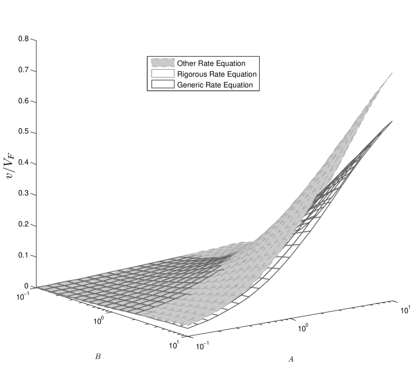
Figure 3: Comparison of different rate equations. Here we take the Bi-Bi ordered mechanism with 8 rate constants as an example. In Ref. [29], a generic bi-substrate rate equation was fitted to the mechanistic rate equation according to a set of data points for the substrates and products concentrations (Conditions CIII in [29], see their Fig. 2). The fit at product concentration $P=Q=0.1$ is considered good. Nevertheless, our proposed generic rate equation, Eq. (2), is capable of reproducing exactly the original rigorous mechanistic rate equation. We note that it is likely the other equation, Eq. (47) may also be cast into the rigorous rate equation using the method shown in Sec. 3.

5.4 Adding modifiers

Modifiers are substances that interact with enzymes to either increase or decrease their catalytic activity. Inhibitors diminish the rate of reaction while activators increase the rate. These are very important in the regulation of metabolic pathways in organisms. For reversible inhibitors, they can be classified into competitive inhibitors and noncompetitive inhibitors. Competitive inhibitors compete with the substrate for binding to the enzyme forming an enzyme-inhibitor complex. The inhibitor does not act on the enzyme-substrate complex once it is formed. For the simple Michaelis-Menten kinetics, the resulting form is

$$\nu=\frac{V_{F}[A]}{K_{A}\left(1+\frac{[I]}{K_{I}}\right)+[A]}\,.$$ (48)

$V_{F}$ is not affected but $K_{A}$ is increased. Non-competitive inhibitors bind with the same affinity to the enzyme and enzyme-substrate complex. It does not change $K_{A}$ but decrease $V_{F}$:

$$\nu=\frac{\left(\frac{1}{1+{[I]}/{K_{I}}}\right)V_{F}[A]}{K_{A}+[A]}\ .$$ (49)

When the affinities are different, the inhibition is called mixed. The net result is to increase in $K_{A}$ and decrease in $V_{F}$. A special case occurs if inhibitor only binds to the enzyme-substrate complex but not to the enzyme, this is called uncompetitive:

$$\nu=\frac{\left(\frac{1}{1+[I]/K_{I}}\right)V_{F}[A]}{\left(\frac{1}{1+[I]/K_{I}}\right)K_{A}+[A]}\,.$$ (50)

To include the effects of inhibitors and activators, we can multiply the unmodified rate equation with a function of the sigmoidal form

$$\frac{1}{1+([I]/a)^{2}}\,,$$ (51)

for an inhibitor, $I$ and

$$\frac{([T]/b)^{2}}{1+([T]/b)^{2}}\,,$$ (52)

for an activator, $T$. The parameter $a$ can be adjusted to match the concentration of the inhibitor at which inhibition becomes significant. The same applies for $b$ in the case of an activator. Other power in the denominator besides 2 can also be used. It is clear that when $V_{F}$ is modified by multiplying the modifier function, this is similar to the case for non-competitive inhibitor in Eq. (49). For the competitive inhibitor case, a suitable choice of $1/K_{I}=(1+\frac{[A]}{K_{A}})/a$ substituted into Eq. (48) gives

$$\nu = \frac{{V_{F}}[A]}{K_{A}\left(1+[I]/K_{I}\right)+[A]}$$ (53)

$$= \frac{V_{F}[A]}{K_{A}\left(1+([I]/a)(1+[A]/K_{A})\right)+[A]}$$

$$= \frac{V_{F}[A]}{(1+[I]/a)(K_{A}+A)}.$$

This is the same form of the inhibitor that we used in Eq. (51). Hence we have shown that both competitive and non-competitive modifiers can generally be accounted for by the modifier form that we used in Eq. (51).

5.5 Uses of proposed rate equation

We have demonstrated above that in situations where exact enzymatic reactions are known, the proposed rate equations are the same as them. In realistic modelling situations, the enzymatic information is typically incomplete. The proposed equations are easy to use because of its simplicity and its parameters or functions are easy to interpret. We elaborate on this observation further below.

Earlier in deriving the generic rate equation (in Sec. 3), we take $V_{F}$, $V_{B}$ and, $K_{i}$’s where $i$ are metabolites in the enzymatic reaction, to be functions of concentrations of metabolities and rate constants in the elementary reactions. We already alluded to the situation of incomplete information, and to the nearly impossibility of obtaining all the relevant in vivo kinetic parameters experimentally. Fortunately, it is well known that the biological networks, either genetic or metabolic, or others, are typically robustly built [2, 5, 6, 8, 11, 16, 17] at functional level. Therefore, very detailed kinetic information may not be necessary in practical situations where we want to simulate a metabolic model under some physiological or functional conditions. We may assign typical values, which may be approximated by constants, to the parameters $V_{F}$, $V_{B}$ and $K_{i}$ in the simulation. Since the operational meaning of these parameters are clear (see below Eq. (2)), we can adjust these parameters in a meaningful way to match physiological conditions.

There is another way to use the proposed enzymatic equation: The compact form of Eq. (2) with approximated values in the kinetic parameters may serve as a starting point to introduce empirical description. Once the values of parameters are fixed, specific experiments to measure them can be performed, and the comparison between theoretical and experimental efforts can lead to better understanding and further study. Clearly, this appears a more straightforward procedure than tuning the rate constants of the elementary reactions (such as the $k_{i}$’s in Eq. (19)) in the original rate equation (such as Eq. (18)). Effectively, the number of parameters in the model is reduced. Can such a strategy be useful? Our experience so far suggests yes.

From a different angle, a third possible use of the proposed enzymatic equation is to regard it as a format to document kinetic parameters from experiments: The form is formally exact, with easy to interpret parameters, and, is ready for computational modeling. In particular, it would be of great value if experimental results on reversible reactions, particularly on the backward velocities, are documented.

We have been using the generic rate equation, Eq. (42) to construct a kinetic model of the metabolism of Methylobacterium extorquens AM1 [41, 42, 43] consisting of about 80 reactions and 80 metabolites. The number of metabolites are the minimum in order to understand the metabolic kinetics at a global level [41, 44]. We are able to find a set of parameters ($V_{F}$, $V_{B}$ and $K_{i}$’s) that give a steady state solution [45]. Our results indicate that the model is robust with respect to variations in kinetic parameters. This is in agreement with observations that quite large errors in kinetic parameters for most of the enzymes have very little effect on the calculated flux [31]. This result is very encouraging as it suggest even larger metabolic network can be built on the same structure for kinetic equations.

Reducing the number of kinetic parameters are also useful when metabolomic data are available for analysis. Under such situation, one could attempt to fit the kinetic parameters to the metabolomic data. One way may be to use Genetic Algorithms to optimize the parameters [46]. Simplifying the number of kinetic parameters cuts the computational effort and makes the problem much more tractable.

6 Conclusions

We have proposed a generic kinetic rate equation. It is shown to be formally identical to rigorous equations and has a considerably simple and generic form. It is already in a form workable for arbitrary number of substrates and products with different stiochiometry. Modifier functions can be added to reflect inhibition and activation. Cooperativity can also be included.

In order to do kinetic modelling according to rigorous equations, numerous parameters need to be measured. Instead, the proposed generic rate equation reduces the required number to the most essential ones, both forward and backward reaction velocities, $V_{F}$, $V_{B}$, and the Michaelis-Menten like constants, $K,K^{\prime}$, for both substrates and products, which have clear chemical and biological meanings. Even if those essential parameters are not always available under appropriate physiological conditions related to living organisms in databases, their adjustments during modelling are much more managable.

The kinetic parameters from enzyme characterization is also dependent on the rate equation being tested. There is an effort underway to ensure uniformity in reporting functional data [47]. The proposed rate equation with only essential parameters may aid such effort to have enzyme characterized. With a database of enzyme parameters for a generic rate equation of the form Eq. (2), the resulting uniformity will make reconstruction of genome scale metabolic networks using kinetic models will become much more feasible.

References

- Hood [2003] L. Hood, Systems biology: Integrating technology, biology, and computation, Mech. Aging Dev. 124, 9 (2003).
- Choi [2007] S. Choi, ed., Introduction to Systems Biology (Humana Press Inc., 2007).
- Yang et al. [2007] K. Yang, W. Ma, H. Liang, Q. Ouyang, C. Tang, and L. Lai, Dynamic simulations on the arachidonic acid metabolic network, PLoS Comput. Biol. 3, 523 (2007).
- Ishii et al. [2007] N. Ishii, K. Nakahigashi, T. Baba, M. Robert, T. Soga, A. Kanai, T. Hirasawa, M. Naba, K. Hirai, A. Hoque, et al., Multiple high-throughput analyses monitor the response of e. coli to perturbations, Science 316, 593 (2007).
- Stephanopoulos et al. [1998] G. N. Stephanopoulos, A. A. Aristidou, and J. Nielsen, Metabolic Engineering: Principles and methodologies (Academic Press, 1998).
- Cortassa et al. [2002] S. Cortassa, M. A. Aon, and A. A. Iglesias, An Introduction to Metabolic and Cellular Engineering (World Scientific, 2002).
- Beard et al. [2002] D. A. Beard, H. Qian, and S. D. Liang, Energy balance for analysis of complex metabolic networks, Biophys. J. 83, 79 (2002).
- Kholodenko and Westerhoff [2004] B. N. Kholodenko and H. V. Westerhoff, eds., Metabolic Engineering in the Post Genomic Era (Norfolk: Horizon Bioscience, 2004).
- Sauro and Kholodenko [2004] H. M. Sauro and B. N. Kholodenko, Quantitative analysis of signaling networks., Prog. Biophys. Mol. Biol. 86, 5 (2004).
- Qian and Bead [2005] H. Qian and D. A. Bead, Thermodynamics of stoichiometric biochemical networks far from equilibrium, Biophys. Chem. 114, 213 (2005).
- Palsson [2006] B. O. Palsson, Systems Biology: properties of reconstructed networks (Cambridge University Press, 2006).
- Bruggeman et al. [2006] F. J. Bruggeman, B. M. Bakker, J. J. Hornberg, and H. V. Westerhoff, Introduction to computational models of biochemical networks, in Computational Systems Biology, edited by A. Kriete and R. Eils (Academic Press, 2006).
- Cha [1968] S. Cha, A simple method for derivation of rate equations for enzyme-catalyzed reactions under the rapid equilibrium assumption or combined assumptions of equilibrium and steady state, J. Biol. Chem. 243, 820 (1968).
- Segel [1975] H. Segel, Enzyme kinetics. Behavior and analysis of rapid equilibrium and steady-state enzyme systems (John Wiley and Sons, 1975).
- Ao [2005] P. Ao, Metabolic network modelling: Including stochastic effects, Comp. Chem. Eng. 29, 2297 (2005).
- Zhu et al. [2004] X.-M. Zhu, L. Yin, L. Hood, and P. Ao, Calculating biological behaviors of epigenetic states in the phage lambda life cycle, Funct. Integr. Genomics 4, 188 (2004).
- Kim and Wang [2007] K. Y. Kim and J. Wang, Potential energy landscape and robustness of a gene regulatory network: Toggle switch, PLoS Comput. Biol. 3, 565 (2007).
- Schomburg et al. [2002] I. Schomburg, A. Chang, and D. Schomburg, BRENDA, enzyme data and metabolic information, Nucleic Acids Res. 30, 47 (2002).
- Schomburg et al. [2004] I. Schomburg, A. Chang, C. Ebeling, M. Gremse, C. Heldt, G. Huhn, and D. Schomburg, BRENDA, the enzyme database: updates and major new developments, Nucleic Acids Res. 32, D431 (2004).
- Kanehisa et al. [2006] M. Kanehisa, S. Goto, M. Hattori, K. F. Aoki-Kinoshita, M. Itoh, S. Kawashima, T. Katayama, M. Araki, and M. Hirakawa, From genomics to chemical genomics: new developments in KEGG, Nucleic Acids Res. 34, D354 (2006).
- Krieger et al. [2004] C. J. Krieger, P. Zhang, M. L. A., A. Wang, S. Paley, M. Arnaud, J. Pick, S. Y. Rhee, and P. D. Karp, MetaCyc: A multiorganism database of metabolic pathways and enzymes, Nucleic Acids Res. 32, D438 (2004).
- Caspi et al. [2006] R. Caspi, H. Foerster, C. A. Fulcher, R. Hopkinson, J. Ingraham, P. Kaipa, M. Krummenacker, S. Paley, J. Pick, S. Y. Rhee, et al., MetaCyc: A multiorganism database of metabolic pathways and enzymes, Nucleic Acids Res. 34, D511 516 (2006).
- Workshop ”Storage and Annotation of Reaction Kinetics Data” [2007] Workshop ”Storage and Annotation of Reaction Kinetics Data”, in In Silico Biology – Supplement (Heidelberg, Germany, 2007), vol. 7, pp. 01–10.
- Poolman et al. [2006] M. G. Poolman, B. K. Bonde, A. Gevorgyan, and D. A. Fell, Challenges to be faced in the reconstruction of metabolic networks from public databases, IEE Proc.-Syst. Biol. 153, 379 (2006).
- Michaelis and Menten [1913] L. Michaelis and M. L. Menten, Kinetics of invertase action, Biochem. Z. 49, 333 (1913).
- English et al. [2006] B. P. English, W. Min, A. M. van Oijen, K. T. Lee, L. Guobin, H. Sun, B. J. Cherayil, S. C. Kou, and X. S. Xie, Ever-fluctuating single enzyme molecules: Michaelis-Menten equation revisited, Nat. Chem. Biol. 2, 87 (2006).
- Briggs and Haldane [1925] G. E. Briggs and J. B. S. Haldane, A note on the kinetics of enzyme actions, Biochem. J. 19, 338 (1925).
- Ciliberto et al. [2007] A. Ciliberto, F. Capuani, and J. J. Tyson, Modeling networks of coupled enzymatic reactions using the total quasi-steady state approximation, PLoS Comput. Biol. 3, 463 (2007).
- Rohwer et al. [2006] J. M. Rohwer, A. J. Hanekom, C. Crous, J. L. Snoep, and J.-H. S. Hofmeyr, Evaluation of a simplified generic bi-substrate rate equation for computational biology, IEE Proc. Syst. Biol. 153, 338 (2006).
- Leskovac et al. [2006] V. Leskovac, S. Trivić, D. Peričin, and J. Kandrač, Deriving the rate equations for product inhibition patterns in bisubstrate enzyme reactions, Journal of Enzyme Inhibition and Medicinal Chemistry 21, 617 (2006).
- Cornish-Bowden and Hofmeyr [2005] A. Cornish-Bowden and J.-H. S. Hofmeyr, Enzymes in context — kinetic characterization of enzymes for systems biology, The Biochemist 27, 11 (2005).
- Morowitz [1992] H. J. Morowitz, Beginnings of Cellular Life: metabolism recapitulates biogenesis (Yale University Press, 1992).
- Cornish-Bowden [2004] A. Cornish-Bowden, Fundamentals of Enzyme Kinetics (Portland Press, 2004).
- Schenll and Maini [2003] S. Schenll and P. K. Maini, A century of enzyme kinetics: Reliability of the and estimates, Comment Theor. Biol. 8, 169 (2003).
- Leskovac [2003] V. Leskovac, Comprehensive Enzyme Kinetics (Kluwer Academic/Plenum, 2003).
- Sorribas et al. [2007] A. Sorribas, B. Hern ndez-Bermejo, E. Vilaprinyo, and R. Alves, Cooperativity and saturation in biochemical networks: A saturable formalism using Taylor series approximations, Biotechnol. Bioeng. 97, 1259 (2007).
- Hill [1910] A. V. Hill, The possible effects of the aggregation of the molecules of haemoglobin on its disassociation curves, J. Physiol. (London) 40, iv (1910).
- Cornish-Bowden and Hofmeyr [1997] A. Cornish-Bowden and J.-H. S. Hofmeyr, The reversible Hill equation: how to incorporate cooperative enzymes into metabolic models, Comp. Appl. Biosci. 13, 377 (1997).
- Heijnen [2005] J. J. Heijnen, Approximative kinetic formats used in metabolic network modeling, Biotech. and Bioeng. 91, 534 (2005).
- Wang et al. [2007] F.-S. Wang, C.-L. Ko, and E. O. Voit, Kinetic modeling using S-systems and lin-log approaches, Biochem. Eng. J. 33, 238 (2007).
- Christoserdova et al. [2003] L. Christoserdova, S.-W. Chen, A. Lapidus, and M. E. Lidstrom, Methylotrophy in methylobacterium extorquens AM1 from a genomic point of view, J. Bacteriol. 185, 2980 (2003).
- Van Dien and Lidstrom [2002] S. J. Van Dien and M. E. Lidstrom, Stiochiometric model for evaluating the metabolic capabilities of the facultative methylotroph methylobacterium extorquens AM1, with application to reconstruction of C(3) and C(4) metabolism, Biotechnol. Bioeng. 78, 296 (2002).
- Van Dien et al. [2003] S. J. Van Dien, T. Strovas, and M. E. Lidstrom, Quantification of central metabolic fluxes in the facultative methylotroph methylobacterium extorquens AM1 using 13C-label tracing and nass spectrometry, Biotechnol. Bioeng. 84, 45 (2003).
- Downs [2006] D. M. Downs, Understanding microbial metabolism, Annu. Rev. Microbiol. 60, 533 (2006).
- Yin et al. [2007] L. Yin, L. W. Lee, X.-M. Zhu, M. E. Lidstrom, and P. Ao, Dynamics of metabolic network: A kinetic model of methylobacterium extorquens AM1, in preparation (2007).
- Nobuyoshi et al. [2005] I. Nobuyoshi, S. Tomoyoshi, N. Takaaki, and T. Masaru, Metabolome analysis and metabolic simulation, Metabolomics 1, 29 (2005).
- Apweiler et al. [2005] R. Apweiler, A. Cornish-Bowden, J. Hofmeyr, C. Kettner, T. Leyh, D. Schomburg, and K. Tipton, The importance of uniformity in reporting protein-function data, Trends Biochem. Sci. 30, 11 (2005).