Parallel marginalization Monte Carlo with applications to conditional path sampling

Abstract

Monte Carlo sampling methods often suffer from long correlation times. Consequently, these methods must be run for many steps to generate an independent sample. In this paper a method is proposed to overcome this difficulty. The method utilizes information from rapidly equilibrating coarse Markov chains that sample marginal distributions of the full system. This is accomplished through exchanges between the full chain and the auxiliary coarse chains. Results of numerical tests on the bridge sampling and filtering/smoothing problems for a stochastic differential equation are presented.

1 Introduction

In spite of substantial effort to improve the efficiency of Markov chain Monte Carlo (MCMC) methods, spatial correlations remain a major impediment. These correlations can severely restrict the possible configurations of a system by imposing complicated relationships between variables. It is well known that judicious elimination of variables by renormalization can reduce long range correlations (see [1, 2]). The remaining variables are distributed according to the marginal distribution,

$$\overline{\pi}\left(x\right)=\int\pi\left(x,y\right)dy,$$

where $\pi\left(x,y\right)$ is the full distribution. Given the values of the $x$ variables and the marginal distribution $\overline{\pi}$ the $y$ variables are distributed according to the conditional distribution

$$\pi\left(y|x\right)=\frac{\pi\left(x,y\right)}{\overline{\pi}\left(x\right)}.$$

For systems exhibiting critical phenomena, the path through the space of distributions taken by marginal distributions under repeated renormalization can yield essential information about critical indices and the location of critical points (see [1, 2]). More generally, because these marginal distributions exhibit shorter correlation lengths and weaker local correlations, they are useful in the acceleration of Markov chain Monte Carlo methods. As explained in the next section, parallel marginalization takes advantage of the shorter correlation lengths present in marginal distributions of the target density.

The use of Monte Carlo updates on lower dimensional spaces is not a new concept. In fact this is a necessary procedure in high dimensions. One simply constructs a chain with steps that preserve the conditional probability density of the full measure. This is usually accomplished by perturbing a few components of the chain while holding all other components of the chain constant. In other words the chain takes steps of the form

$$Y^{n+1}=(x_{1},\dots,x_{i-1},x_{i}+\epsilon,x_{i+1},\dots,x_{d})$$

where

$$Y^{n}=(x_{1},\dots,x_{d})$$

and the move preserves $\pi(x_{i}|x_{1},\dots,x_{i-1},x_{i+1},\dots,x_{d}).$ There have been many important attempts to use proposals in more general sets of projected coordinates. The multi-grid Monte Carlo method presented in [3, 4] is one such method. These techniques do not incorporate marginal densities.

In [5], Brandt and Ron propose a multi-grid method which approximates successive marginal distributions of the Ising model and then uses these approximations to generate large scale movements of the Markov chain sampling the full joint distribution of all variables. Their method, while demonstrating the efficacy of incorporating information from successive marginal distributions, suffers from two limitations. First, the method used to approximate the marginal distributions is specific to a small class of problems. For example, it cannot be easily generalized to systems in continuous spaces. Second, information from the approximate marginal distributions is adopted by the Markov chain in a way which does not preserve the target distribution of all variables.

The design of a generally applicable method which approximates the marginal distributions was addressed in [6, 7] by Chorin, and in [8] by Stinis. Both authors approximate the renormalized Hamiltonian of the system given by the formula,

$$\overline{\mathcal{H}}\left(x\right)=-\log\int\pi\left(x,y\right)dy.$$

Thus $\exp\left(-\overline{\mathcal{H}}\left(x\right)\right)$ is the marginal distribution of the $x$ variables. Chorin determines the coefficients in an expansion of $\overline{\mathcal{H}}\left(x\right)$ by first expanding the derivatives $\frac{\partial\overline{\mathcal{H}}\left(x\right)}{\partial x}$, which can be expressed as conditional expectations with respect to the full distribution. Stinis shows that a maximum likelihood approximation to the renormalized Hamiltonian can be found by minimizing the error in the expectations of the basis functions in an expansion of $\overline{\mathcal{H}}\left(x\right)$. For applications of related ideas to MCMC simulations see [9] and [10].

Two Parallel marginalization algorithms are developed in the next section along with propositions that guarantee that the resulting Markov chains satisfy the detailed balance condition. In the final section the conditional path sampling problem is described and numerical results are presented for the bridge sampling and smoothing/filtering problems. A brief introduction to parallel marginalization can be found in [11].

2 Parallel marginalization

In this section, it is assumed that appropriate approximate marginal distributions are available. How to find these marginal distributions depends on the application and will be discussed here only in the context of the examples presented in this paper. A new Markov chain Monte Carlo method is introduced which uses approximate marginal distributions of the target distribution to accelerate sampling. Auxiliary Markov chains that sample approximate marginal distributions are evolved simultaneously with the Markov chain that samples the distribution of interest. By swapping their configurations, these auxiliary chains pass information between themselves and with the chain sampling the original distribution.

Assume that the system of interest has a probability density, $\pi_{0}(x_{0})$, where $x_{0}$ lies in some space $E.$ Suppose further that, by the Metropolis-Hastings or any other method (see [12]), one can construct a Markov chain, $Y_{0}^{n}\in E$, which has $\pi_{0}$ as its stationary measure. That is, for two points $x_{0},y_{0}\in E$

$$\int\tau_{0}(y_{0}|x_{0})\pi_{0}(x_{0})\ dx_{0}=\pi_{0}(y_{0})$$

where $\tau_{0}(y_{0}|x_{0})$ is the probability density of a move to $\left\{Y_{0}^{n+1}=y_{0}\right\}$ given that $\left\{Y_{0}^{n}=x_{0}\right\}$. Here, $n$ is the algorithmic step.

In order to take advantage of the shorter spatial correlations exhibited by marginal distributions of $\pi_{0}$, a collection of lower dimensional Markov chains which approximately sample marginal distributions of $\pi_{0}$ is considered. Suppose the random variable $X_{0}$ has $d_{0}$ components. Divide these into two subsets,

$$X_{0}=\left(\widehat{X}_{0},\widetilde{X}_{0}\right),$$

where $\widehat{X}_{0}$ has $d_{1}$ components and $\widetilde{X}_{0}$ has $d_{0}-d_{1}$ components. Recall that the $\widehat{X}_{0}$ variables are distributed according to the marginal density,

$$\overline{\pi}_{0}(\hat{x}_{0})=\int\pi_{0}(\hat{x}_{0},\tilde{x}_{0})d\tilde{x}_{0}$$ (1)

and that given the value of the $\widehat{X}_{0}$ variables, the $\widetilde{X}_{0}$ variables are distributed according to the conditional density,

$$\pi(\tilde{x}_{0}|\hat{x}_{0})=\frac{\pi_{0}(\hat{x}_{0},\tilde{x}_{0})}{\overline{\pi}_{0}(\hat{x}_{0})}$$ (2)

Label the domain of the $\widehat{X}_{0}$ variables $E_{1}$. Suppose further that an approximation to the marginal distribution of the $\widehat{X}_{0}$ variables,

$$\pi_{1}\left(\hat{x}_{0}\right)\approx\overline{\pi}_{0}\left(\hat{x}_{0}\right)$$

is available. The sense in which $\pi_{1}$ approximates $\overline{\pi}_{0}$ is intentionally left vague. In applications of parallel marginalization the accuracy of the approximation manifests itself through an acceptance rate.

Now let $X_{1}\in E_{1}$ be independent of the $X_{0}$ random variables and drawn from $\pi_{1}\left(\widehat{x}_{0}\right)$. Notice that $X_{1}$ represents the same physical variables as $\widehat{X}_{0}$ though its probability density is not the exact marginal density. Continue in this way to remove variables from the system by decomposing $X_{l}\in E_{l}$ into proper subsets as

$$X_{l}=\left(\widehat{X}_{l},\widetilde{X}_{l}\right)$$

and defining $X_{l+1}\in E_{l+1}$ to be independent of the $\left\{X_{0},\dots,X_{l}\right\}$ random variables and drawn from an approximation $\pi_{l+1}$ to $\overline{\pi}_{l}\left(\hat{x}_{l}\right)$. Clearly each $X_{l+1}$ represents fewer physical variables than $X_{l}$.

Just as one can construct a Markov chain $Y^{n}_{0}\in E_{0}$ to sample $X_{0}$, one can also construct Markov chains $Y_{l}^{n}\in E_{l}$ to sample $\pi_{l}$. In other words, for each $Y_{l}^{n}$ choose a transition probability density $\tau_{l},$ such that

$$\int\tau_{l}(y_{l}|x_{l})\pi_{l}\left(x_{l}\right)dx_{l}=\pi_{l}\left(y_{l}\right)$$

for all $i.$

The chains $Y^{n}_{l}$ can be arranged in parallel to yield a larger Markov chain,

$$Y^{n}=\left(Y^{n}_{0},\dots,Y^{n}_{L}\right)\in E_{0}\times\dots\times E_{L}.$$

The probability density of a move to $\left\{Y^{n+1}=y\right\}$ given that $\left\{Y^{n}=x\right\}$ for $x,y\in E_{0}\times\dots\times E_{L}$ is given by

$$\tau(y|x)=\prod_{l=0}^{L}\tau_{l}(y_{l}|x_{l}).$$ (3)

Since

$$\int\left(\tau(y|x)\prod_{l=0}^{L}\pi_{l}\left(x_{l}\right)\right)\ dx_{0}\dots dx_{L}=\prod_{l=0}^{L}\pi_{l}\left(y_{l}\right)$$

the stationary distribution of $Y^{n}$ is

$$\Pi\left(x_{0},\dots,x_{L}\right)=\pi_{0}\left(x_{0}\right)\dots\pi_{L}\left(x_{L}\right).$$

The next step in the construction is to allow interactions between the chains $Y_{l}^{n}$ and to thereby pass information from the rapidly equilibrating chains on the lower dimensional spaces (large $l$) down to the chain on the original space ($l=0$). This is accomplished by swap moves. In a swap move between levels $l$ and $l+1$, a subset, $\hat{x}_{l}\in E_{l+1}$, of the $x_{l}$ variables is exchanged with the $x_{l+1}\in E_{l+1}$ variables. The remaining $\tilde{x}_{l}$ variables are resampled from the conditional distribution $\pi_{l}\left(\tilde{x}_{l}|x_{l+1}\right)$. For the full chain, this swap takes the form of a move from $\left\{Y^{n}=x\right\}$ to $\left\{Y^{n+1}=y\right\}$ where

$$x=\left(\dots,\hat{x}_{l},\tilde{x}_{l},x_{l+1},\dots\right)$$

and

$$y=\left(\dots,x_{l+1},\tilde{y}_{l},\hat{x}_{l},\dots\right).$$

The $\tilde{y}_{l}$ variables are drawn from $\pi_{l}\left(\tilde{x}_{l}|x_{l+1}\right)$ and the ellipses represent components of $Y^{n}$ that remain unchanged in the transition.

If these swaps are undertaken unconditionally, the resulting chain may equilibrate rapidly, but will not, in general, preserve the product distribution $\Pi$. To remedy this the swap acceptance probability

$$A_{l}=\min\biggl{\{}1,\ \frac{\overline{\pi}_{l}(x_{l+1})\pi_{l+1}(\hat{x}_{l})}{\overline{\pi}_{l}(\hat{x}_{l})\pi_{l+1}(x_{l+1})}\biggr{\}}$$ (4)

is introduced. Recall that $\overline{\pi}_{l}$ is the function resulting from the integration of $\pi_{l}$ over the $\tilde{x}_{l}$ variables as in equation (1). Given that $\left\{Y^{n}=x\right\}$, the probability density of $\left\{Y^{n+1}=y\right\}$, after the proposal and either acceptance with probability $A_{l}$ or rejection with probability $1-A_{l}$, of a swap move, is given by

$$\psi_{l}\left(y|x\right)=\left(1-A_{l}\right)\ \prod\delta_{\left\{y_{j}=x_{j}\right\}}\\ +A_{l}\ \pi_{l}(\tilde{y}_{l}|x_{l+1})\ \delta_{\left\{\left(\hat{y}_{l},y_{l+1}\right)=\left(x_{l+1},\hat{x}_{l}\right)\right\}}\prod_{j\notin\left\{l,l+1\right\}}\delta_{\left\{y_{j}=x_{j}\right\}}$$

for $x,y\in E_{0}\times\dots\times E_{L}$. $\delta$ is the Dirac delta function.

We have the following proposition.

Proposition 1.

The transition probabilities $\psi_{l}$ satisfy the detailed balance condition for the measure $\Pi,$ i.e.

$$\Pi(x)\ \psi_{l}\left(y|x\right)=\Pi(y)\ \psi_{l}\left(x|y\right)$$

where $x,y\in E_{0}\times\dots\times E_{L}.$

Proof.

Fix $x,y\in E_{0}\times\dots\times E_{L}$ such that $x\neq y$.

$$\Pi(x)\ \psi_{l}\left(y|x\right)=\left(\prod_{j\notin\left\{l,l+1\right\}}\pi_{j}\left(x_{j}\right)\delta_{\left\{y_{j}=x_{j}\right\}}\right)\pi_{l}\left(x_{l}\right)\pi_{l+1}\left(x_{l+1}\right)\\ \times\left(\left(1-A_{l}\right)\ \delta_{\left\{\left(y_{l},y_{l+1}\right)=\left(x_{l},x_{l+1}\right)\right\}}+A_{l}\ \pi_{l}(\tilde{y}_{l}|x_{l+1})\ \delta_{\left\{\left(\hat{y}_{l},y_{l+1}\right)=\left(x_{l+1},\hat{x}_{l}\right)\right\}}\right)$$

When $x\neq y$ $\left(\Pi(x)\psi_{l}\left(y|x\right)\right)$ and $\left(\Pi(y)\psi_{l}\left(x|y\right)\right)$ are both zero unless $x_{j}=y_{j}$ for all $j$ except $l$ and $l+1$ and $\left(\hat{y}_{l},y_{l+1}\right)=\left(x_{l+1},\hat{x}_{l}\right)$. Therefore it is enough to check that the function

$$R\left(\left(x_{l},x_{l+1}\right),\left(y_{l},y_{l+1}\right)\right)=\pi_{l}\left(x_{l}\right)\pi_{l+1}\left(x_{l+1}\right)\pi_{l}\left(\tilde{y}_{l}|x_{l+1}\right)\ A_{l}$$

is symmetric in $\left(x_{l},x_{l+1}\right)$ and $\left(y_{l},y_{l+1}\right)$ when $\left(\hat{y}_{l},y_{l+1}\right)=\left(x_{l+1},\hat{x}_{l}\right)$. Plugging in the definition of $A_{l},$

$$R=\pi_{l}\left(x_{l}\right)\pi_{l+1}\left(x_{l+1}\right)\pi_{l}\left(\tilde{y}_{l}|x_{l+1}\right)\ \min\biggl{\{}1,\ \frac{\overline{\pi}_{l}(x_{l+1})\pi_{l+1}(\hat{x}_{l})}{\overline{\pi}_{l}(\hat{x}_{l})\pi_{l+1}(x_{l+1})}\biggr{\}}$$

Rearranging terms gives,

$$R =\pi_{l}\left(x_{l}\right)\pi_{l+1}\left(x_{l+1}\right)\pi_{l}\left(\tilde{y}_{l}|x_{l+1}\right)\overline{\pi}_{l}\left(x_{l+1}\right)\pi_{l+1}\left(y_{l+1}\right)$$

$$\hskip 24.0pt\times\min\biggl{\{}\frac{1}{\overline{\pi}_{l}(x_{l+1})\pi_{l+1}(y_{l+1})},\ \frac{1}{\overline{\pi}_{l}(y_{l+1})\pi_{l+1}(x_{l+1})}\biggr{\}}$$

Recall from (2), that $\pi_{l}(\tilde{y}_{l}|x_{l+1})\overline{\pi}_{l}(x_{l+1})=\pi_{l}(x_{l+1},\tilde{y}_{l}).$ Therefore, since $x_{l+1}=\hat{y}_{l},$

$$R =\pi_{l}\left(x_{l}\right)\pi_{l+1}\left(x_{l+1}\right)\pi_{l}\left(y_{l}\right)\pi_{l+1}\left(y_{l+1}\right)$$

$$\hskip 24.0pt\times\min\biggl{\{}\frac{1}{\overline{\pi}_{l}(x_{l+1})\pi_{l+1}(y_{l+1})},\ \frac{1}{\overline{\pi}_{l}(y_{l+1})\pi_{l+1}(x_{l+1})}\biggr{\}}$$

The final formula is clearly symmetric in $\left(x_{l},x_{l+1}\right)$ and $\left(y_{l},y_{l+1}\right)$. ∎

The detailed balance condition stipulates that the probability of observing a transition $x\rightarrow y$ is equal to that of observing a transition $y\rightarrow x$ and guarantees that the resulting Markov Chain preserves the distribution $\Pi$. If the chain is also Harris recurrent then averages over a trajectory of $Y^{n}$ will converge to averages over $\Pi$. In fact, chains generated by swaps as described above cannot be recurrent and must be combined with another transition rule to generate a convergent Markov chain. Since

$$\pi_{0}(x_{0})=\int\Pi(x_{0},\dots,x_{L})\ dx_{1}\dots dx_{L},$$

if $Y^{n}$ is Harris recurrent with invariant distribution $\Pi$, averages over $\pi_{0}$ can be calculated by taking averages over the trajectories of the first $d_{0}$ components of $Y^{n}$.

2.1 Approximation of acceptance probabilities

Notice that the formula (4) for $A_{l}$ requires the evaluation of $\overline{\pi}_{l}$ at the points $\hat{x}_{l},x_{l+1}\in E_{l+1}.$ While the approximation of $\overline{\pi}_{l}$ by functions on $E_{l+1}$ is in general a very difficult problem, its evaluation at a single point is often not terribly demanding. In fact, in many cases, including the examples in Chapter 3, the $\widehat{X}_{l}$ variables can be chosen so that the remaining $\widetilde{X}_{l}$ variables are conditionally independent given $\widehat{X}_{l}.$

Despite this mitigating factor, the requirement that $\overline{\pi}_{l}$ be evaluated before acceptance of any swap is inconvenient. Fortunately, and somewhat surprisingly, this requirement is not necessary. In fact, standard strategies for approximating the point values of the marginals yield Markov chains that also preserve the target measure. Thus even a poor estimate of the ratio appearing in (4) can give rise to a method that is exact in the sense that the resulting Markov chain will asymptotically sample the target measure.

Before moving on to the description of the resulting Markov chain Monte Carlo algorithms consider briefly the general problem of evaluating marginal densities. Let $p_{1}(x,y)$ and $p_{2}(x,y)$ be the densities of two equivalent measures with marginal densities,

$$\overline{p}_{1}(x)=\int p_{1}(x,y)dy$$

and

$$\overline{p}_{2}(x)=\int p_{2}(x,y)dy$$

respectively. For any integrable function $\gamma(x,y),$

$$\mathbf{E}_{p_{1}}\left[\gamma\left(X,Y\right)p_{2}\left(X,Y\right)|\left\{X=x\right\}\right] =\int\gamma(x,y)p_{2}(x,y)p_{1}(y|x)dy$$

$$=\frac{\overline{p}_{2}(x)}{\overline{p}_{1}(x)}\int\gamma(x,y)p_{2}(y|x)p_{1}(x,y)dy$$

$$=\frac{\overline{p}_{2}(x)}{\overline{p}_{1}(x)}\mathbf{E}_{p_{2}}\left[\gamma\left(X,Y\right)p_{1}\left(X,Y\right)|\left\{X=x\right\}\right]$$

Thus given $\overline{p}_{2}(x),$ the value of $\overline{p}_{1}$ at $x$ can be obtained through the formula,

$$\overline{p}_{1}(x)=\overline{p}_{2}(x)\frac{\mathbf{E}_{p_{2}}\left[\gamma\left(X,Y\right)p_{1}\left(X,Y\right)|\left\{X=x\right\}\right]}{\mathbf{E}_{p_{1}}\left[\gamma\left(X,Y\right)p_{2}\left(X,Y\right)|\left\{X=x\right\}\right]}$$ (5)

Of course, the usual importance sampling concerns apply here. In particular, the approximation of the conditional expectations in (5) will be much easier when $Y$ lives in a lower dimensional space.

Similar approximations can be inserted into our acceptance probabilities $A_{l}$ in place of the ratio $\frac{\overline{\pi}_{l}(x_{l+1})}{\overline{\pi}_{l}(\hat{x}_{l})}.$ For example, if $p_{l}(\tilde{x}_{l}|\hat{x}_{l})$ is a reference density approximating $\pi_{l}(\tilde{x}_{l}|\hat{x}_{l}),$ then the choice

$$\gamma(\hat{x}_{l},\tilde{x}_{l})=\frac{1}{p_{l}(\hat{x}_{l},\tilde{x}_{l})}$$

yields

$$\overline{\pi}_{l}(\hat{x})\approx\overline{p}_{l}(\hat{x})\frac{1}{M}\sum\frac{\pi_{l}\left(\hat{x}_{l},V^{j}\right)}{p_{l}\left(\hat{x},V^{j}\right)}=\frac{1}{M}\sum\frac{\pi_{l}\left(\hat{x}_{l},V^{j}\right)}{p_{l}\left(V^{j}|\hat{x}_{l}\right)}$$ (6)

where the $V^{j}$ are samples from $p_{l}(\tilde{x}_{l}|\hat{x}_{l}).$ Thus if $U^{j}$ are samples from $p_{l}(\tilde{x}_{l}|x_{l+1}),$ then

$$\frac{\frac{1}{M}\sum_{j=1}^{M}\frac{\pi_{l}\left(x_{l+1},U^{j}\right)}{p_{l}\left(U^{j}|x_{l+1}\right)}}{\frac{1}{M}\sum_{j=1}^{M}\frac{\pi_{l}\left(\hat{x}_{l},V^{j}\right)}{p_{l}\left(V^{j}|\hat{x}_{l}\right)}}\xrightarrow[M\rightarrow\infty]{a.s.}\frac{\mathbf{E}_{p_{l}}\left[\frac{\pi_{l}\left(x_{l+1},\widetilde{X}_{l}\right)}{p_{l}\left(\widetilde{X}_{l}|x_{l+1}\right)}\ |\left\{\widehat{X}_{l}=x_{l+1}\right\}\right]}{\mathbf{E}_{p_{l}}\left[\frac{\pi_{l}\left(\hat{x}_{l},\widetilde{X}_{l}\right)}{p_{l}\left(\widetilde{X}_{l}|\hat{x}_{l}\right)}\ |\left\{\widehat{X}_{l}=\hat{x}_{l}\right\}\right]}=\frac{\overline{\pi}_{l}(x_{l+1})}{\overline{\pi}_{l}(\hat{x}_{l})}$$

In the numerical examples presented here, $p_{l}(\ \cdot\ |\hat{x}_{l})$ is a Gaussian approximation of $\pi_{l}(\tilde{x}_{l}|\hat{x}_{l})$. How $p_{l}$ is chosen depends on the problem at hand (see numerical examples below). In general $p_{l}(\ \cdot\ |\hat{x}_{l})$ should be easily evaluated and independently sampled, and it should “cover” $\pi_{l}(\ \cdot\ |\hat{x}_{l})$ in the sense that regions where $\pi_{l}(\ \cdot\ |\hat{x}_{l})$ is not negligible should be contained in regions where $p_{l}(\ \cdot\ |\hat{x}_{l})$ is not negligible. In the case mentioned above that the $\widehat{X}_{l}$ variables can be chosen so that the remaining $\widetilde{X}_{l}$ variables are conditionally independent given $\widehat{X}_{l}$ the conditional density $\pi_{l}(\tilde{x}_{l}|\hat{x}_{l})$ can be written as a product of many low dimensional densities. As mentioned above, the problem of finding a reference density for importance sampling is much simpler in low dimensional spaces.

The following algorithm results from replacing $A_{l}$ in (4) with approximation of the form (6). Assume that the current position of the chain is $\left\{Y^{n}=x\right\}$ where

$$x=\left(\dots,\hat{x}_{l},\tilde{x}_{l},x_{l+1},\dots\right).$$

Algorithm 1 will result in either $\left\{Y^{n+1}=x\right\}$ or $\left\{Y^{n+1}=y\right\}$ where

$$y=\left(\dots,x_{l+1},\tilde{y}_{l},\hat{x}_{l},\dots\right)$$

and $\tilde{y}_{l}$ is approximately drawn from $\pi_{l}\left(\tilde{x}_{l}|x_{l+1}\right).$

Algorithm 1 (Parallel Marginalization 1).

The chain moves from $Y^{n}$ to $Y^{n+1}$ as follows:

1. Let $U^{j}$ for $j=1,\dots,M$ be independent random variables sampled from $p_{l}(\ \cdot\ |x_{l+1})$ (recall that the swap is between $\hat{x}_{l}$ and ${x_{l+1}}$ which are both in $E_{l+1}$).

2. Evaluate the weights

   $$W_{U}^{j}=\frac{\pi_{l}\left(x_{l+1},U^{j}\right)}{p_{l}\left(U^{j}|\ x_{l+1}\right)}.$$

   The choice of $p_{l}$ made above affects the variance of these weights, and therefore the variance of the acceptance probability below.

3. Draw the random index $J\in\left\{1,\dots,M\right\}$ according to the probabilities

   $$\mathbf{P}\left[J=j\right]=\frac{W_{U}^{j}}{\sum_{m=1}^{M}W_{U}^{m}}.$$

   Set $\widetilde{Y}^{\prime}=U^{J}.$ Notice that $\widetilde{Y}^{\prime}$ is an approximate sample from $\pi_{l}(\ \cdot\ |x_{l+1}).$

4. Let $V^{J}=\tilde{x}_{l}$ and draw $V^{j}$ for $j\neq J$ independently from $p_{l}(\ \cdot\ |\hat{x}_{l}),$ Notice that the $U^{j}$ variables depend on $x_{l+1}$ while the $V^{j}$ variables depend on $\hat{x}_{l}$.

5. Define the weights

   $$W_{V}^{j}=\frac{\pi_{l}\left(\hat{x}_{l},V^{j}\right)}{p_{l}\left(V^{j}|\hat{x}_{l}\right)}$$

6. Set

   $$Y^{n+1}=\left(\dots,x_{l+1},\widetilde{Y}^{\prime},\hat{x}_{l},\dots\right)$$

   with probability

   $$A^{M}_{l}=\min\biggl{\{}1,\ \frac{\pi_{l+1}(\hat{x}_{l})\sum_{j=1}^{M}W^{j}_{U}}{\pi_{l+1}(x_{l+1})\sum_{j=1}^{M}W^{j}_{V}}\biggr{\}}$$ (7)

   and

   $$Y^{n+1}=Y^{n}=\left(\dots,\hat{x}_{l},\tilde{x}_{l},x_{l+1},\dots\right)$$

   with probability $1-A^{M}_{l}$.

The transition probability density for the above swap move from $x$ to $y$ for $x,y\in E_{0}\times\dots\times E_{L}$is given by

$$\psi^{M}_{l}(y|x)=\mathbf{P}\left[\left\{\text{Swap is rejected}\right\}\right]\ \prod\delta_{\left\{y_{j}=x_{j}\right\}}\\ +\mathbf{P}\left[\left\{\text{Swap is accepted}\right\}\cap\left\{\widetilde{Y}^{\prime}=\tilde{y}_{l}\right\}\right]\\ \times\delta_{\left\{\left(\hat{y}_{l},y_{l+1}\right)=\left(x_{l+1},\hat{x}_{l}\right)\right\}}\prod_{j\notin\left\{i,i+1\right\}}\delta_{\left\{y_{j}=x_{j}\right\}},$$

where $\delta$ is again the Dirac delta function. Notice that to find the probability density $\mathbf{P}\left[\left\{\text{Swap is accepted}\right\}\cap\left\{\widetilde{Y}^{\prime}=\tilde{y}_{l}\right\}\right]$ one must integrate over the possible values of the $U^{j}$ and $V^{j}$ variables. Since $\pi_{l}$ appears in the integrand it is not possible, in general, to evaluate the integral. However, as indicated in the proof of the next proposition, it is not necessary to evaluate this density to show that the method converges.

While the preceding swap move corresponds to a method for approximating the ratio

$$\frac{\overline{\pi}_{l}(x_{l+1})}{\overline{\pi}_{l}(\hat{x}_{l})}$$

appearing in formula (4) for $A_{l},$ it also has similarities with the multiple-try Metropolis method, presented in [13, 14], that uses multiple suggestion samples to improve acceptance rates of standard MCMC methods. In fact the proof of the following proposition is motivated by the proof of the detailed balance condition for the multiple try method.

Proposition 2.

The transition probabilities $\psi^{M}_{l}$ satisfy the detailed balance condition for the measure $\Pi.$

Proof.

For $x,y\in E_{0}\times\dots\times E_{L}$ such that $x\neq y$,

$$\Pi(x)\ \psi^{M}_{l}(y|x)=\Pi(x)\ \mathbf{P}\left[\left\{\text{Swap is accepted}\right\}\cap\left\{\widetilde{Y}^{\prime}=\tilde{y}_{l}\right\}\right]\\ \times\delta_{\left\{\left(\hat{y}_{l},y_{l+1}\right)=\left(x_{l+1},\hat{x}_{l}\right)\right\}}\prod_{j\notin\left\{i,i+1\right\}}\delta_{\left\{y_{j}=x_{j}\right\}},$$

As in the previous proof it can be assumed that $x_{j}=y_{j}$ for all $j$ except $l$ and $l+1$ and $\left(\hat{y}_{l},y_{l+1}\right)=\left(x_{l+1},\hat{x}_{l}\right)$. Since in this case $\pi(x_{j})=\pi(y_{j})$ for all $j\notin\left\{l,l+1\right\},$ it remains to show that if $\left(\hat{y}_{l},y_{l+1}\right)=\left(x_{l+1},\hat{x}_{l}\right)$ then

$$R\left(\left(x_{l},x_{l+1}\right),\left(y_{l},y_{l+1}\right)\right)=\pi_{l}\left(x_{l}\right)\pi_{l+1}\left(x_{l+1}\right)\\ \times\mathbf{P}\left[\left\{\text{Swap is accepted}\right\}\cap\left\{\widetilde{Y}^{n+1}_{l}=\tilde{y}_{l}\right\}\right]$$

is symmetric in $\left(x_{l},x_{l+1}\right)$ and $\left(y_{l},y_{l+1}\right)$. Define a random index $J\in\left\{1,\dots,M\right\}$ by the relation $\tilde{y}_{l}=U^{J}.$ Then, since the $U^{j}$ are $i.i.d.$,

$$\mathbf{P}\left[\left\{\text{Swap is accepted}\right\}\cap\left\{\widetilde{Y}^{\prime}=\tilde{y}_{l}\right\}\right]=$$

$$\sum_{j=1}^{M}\mathbf{P}\left[\left\{\text{Swap is accepted}\right\}\cap\left\{\tilde{y}_{l}=U^{j}\right\}\cap\left\{J=j\right\}\right]$$

$$=M\ \mathbf{P}\left[\left\{\text{Swap is accepted}\right\}\cap\left\{\tilde{y}_{l}=U^{1}\right\}\cap\left\{J=1\right\}\right]$$

Thus,

$$R\left(\left(x_{l},x_{l+1}\right),\left(y_{l},y_{l+1}\right)\right)= \ M\ \pi_{l}\left(x_{l}\right)\pi_{l+1}\left(x_{l+1}\right)$$

$$\times\mathbf{P}\left[\left\{\text{Swap is accepted}\right\}\cap\left\{\tilde{y}_{l}=U^{1}\right\}\cap\left\{J=1\right\}\right]$$

Writing out the density on the right of this relation gives,

$$R= \ M\ \pi_{l}\left(x_{l}\right)\pi_{l+1}\left(x_{l+1}\right)\int\min\biggl{\{}1,\ \frac{\pi_{l+1}(\hat{x}_{l})\sum_{j=1}^{M}W^{j}_{U}}{\pi_{l+1}(x_{l+1})\sum_{j=1}^{M}W^{j}_{V}}\biggr{\}}\frac{\frac{\pi_{l}\left(x_{l+1},u^{1}\right)}{p\left(u^{1}|x_{l+1}\right)}}{\sum_{j=1}^{M}W^{j}_{U}}$$

$$\hskip 24.0pt\times p\left(u^{1}|x_{l+1}\right)\prod_{j>1}p\left(u^{j}|x_{l+1}\right)p\left(v^{j}|\hat{x}_{l}\right)du^{j}dv^{j}$$

Replacing $u^{1}$ by $\tilde{y}_{l}$ and rearranging gives,

$$R= \ M\ \pi_{l}\left(x_{l}\right)\pi_{l+1}\left(x_{l+1}\right)\pi_{l}\left(x_{l+1},\tilde{y}_{l}\right)\pi_{l+1}\left(\hat{x}_{l}\right)$$

$$\hskip 24.0pt\times\int\min\biggl{\{}\frac{1}{\pi_{l+1}\left(\hat{x}_{l}\right)\sum_{j=1}^{M}W^{j}_{U}},\ \frac{1}{\pi_{l+1}(x_{l+1})\sum_{j=1}^{M}W^{j}_{V}}\biggr{\}}$$

$$\hskip 48.0pt\times\prod_{j>1}p\left(u^{j}|x_{l+1}\right)p\left(v^{j}|\hat{x}_{l}\right)du^{j}dv^{j}.$$

Since $x_{l+1}=\hat{y}_{l},$ $\pi_{l}(x_{l+1},\tilde{y}_{l})=\pi_{l}(y_{l}).$ Therefore, after replacing $\hat{x}_{l}$ by $y_{l+1},$

$$R= \ M\ \pi_{l}\left(x_{l}\right)\pi_{l+1}\left(x_{l+1}\right)\pi_{l}\left(y_{l}\right)\pi_{l+1}\left(y_{l+1}\right)$$

$$\hskip 24.0pt\times\int\min\biggl{\{}\frac{1}{\pi_{l+1}\left(y_{l+1}\right)\sum_{j=1}^{M}W^{j}_{U}},\ \frac{1}{\pi_{l+1}(x_{l+1})\sum_{j=1}^{M}W^{j}_{V}}\biggr{\}}$$

$$\hskip 48.0pt\times\prod_{j>1}p\left(u^{j}|x_{l+1}\right)p\left(v^{j}|y_{l+1}\right)du^{j}dv^{j}.$$

which is symmetric in $\left(x_{l},x_{l+1}\right)$ and $\left(y_{l},y_{l+1}\right)$. ∎

For small values of $M$ in (13), calculation of the swap acceptance probabilities is very cheap. However, higher values of $M$ may improve the acceptance rates. For example, if the $\pi_{l}$ for $l>0$ are exact marginals of $\pi_{0},$ then $A_{l}\equiv 1$ while $A^{M}_{l}\leq 1.$ In practice one has to balance the speed of evaluating $A_{l}^{M}$ for small $M$ with the possible higher acceptance rates for $M$ large.

In analogy again with the multiple-try method, the above algorithm can be generalized to include correlated samples $U^{j}$ and $V^{j}$. This generalization is useful because it allows reference densities that cannot be independently sampled. Again consider a transition from $\left\{Y^{n}=x\right\}$ where

$$x=\left(\dots,\hat{x}_{l},\tilde{x}_{l},x_{l+1},\dots\right)$$

to either $\left\{Y^{n+1}=x\right\}$ or $\left\{Y^{n+1}=y\right\}$ where

$$y=\left(\dots,x_{l+1},\tilde{y}_{l},\hat{x}_{l},\dots\right).$$

First choose some reference transition densities $p_{l}^{j}\left(u^{j}|\left(u^{0},\dots,u^{j-1}\right),\ \hat{x}_{l}\right)$ that sample a variable $U^{j}$ given the previous $j-1$ samples and the value of the $\hat{x}_{l}$ variables. Let

$$p_{l}^{j}\left((u^{k+1},\dots,u^{j})|(u^{0},\dots,u^{k}),\ \hat{x}_{l}\right)=\prod_{k<m\leq j}p_{l}^{m}\left(u^{m}|(u^{0},\dots,u^{m-1}),\ \hat{x}_{l}\right).$$ (8)

For example, one might choose the $p^{j}_{l}$ to be Markov transition kernels associated with some Markov chain Monte Carlo method with stationary measure $\pi_{l}(\tilde{x}_{l}|\hat{x}_{l}).$ Also let $\lambda^{j}\left((u^{0},\dots,u^{j}),\ \hat{x}_{l},x_{l+1}\right)$ be any function satisfying the relation

$$\lambda^{j}\left((u^{0},\dots,u^{j}),\ \hat{x}_{l},x_{l+1}\right)=\lambda^{j}\left((u^{j},\dots,u^{0}),\ x_{l+1},\hat{x}_{l}\right)$$

Algorithm 2 (Parallel Marginalization 2).

We move the chain from $Y^{n}$ to $Y^{n+1}$ as follows:

1. For $j=1,\dots,M$ sample $U^{j}$ from $p_{l}^{j}\left(\ \cdot\ |(\tilde{x}_{l},U^{1},\dots,U^{j-1}),\ x_{l+1}\right).$ Notice the conditioning on the value $\widehat{X}_{l}=x_{l+1}$.

2. Define the weights

   $$W_{U}^{j} =\pi_{l}\left(U^{j},x_{l+1}\right)p_{l}^{j}\left(\left(U^{j-1},\dots,U^{1},\tilde{x}_{l}\right)|U^{j},\ \hat{x}_{l}\right)$$

   $$\hskip 24.0pt\times\lambda^{j}\left(\left(\tilde{x}_{l},U^{1},\dots,U^{j}\right),\ \hat{x}_{l},x_{l+1}\right).$$

   Notice the reversal in the ordering of the $U^{j}$ and the conditioning on $\widehat{X}_{l}=\hat{x}_{l}$.

3. Choose the random index $J\in\left\{1,\dots,M\right\}$ according to the probabilities

   $$\mathbf{P}\left[J=j\right]=\frac{W_{U}^{j}}{\sum_{m=1}^{M}W_{U}^{m}}.$$

   Set $\widetilde{Y}^{\prime}=U^{J}.$

4. Let $V^{J}=\tilde{x}_{l}$ and for $j=1,\dots,J-1$ let $V^{j}=U^{J-j}$. For $j=J+1,\dots,M$ sample $V^{j}$ from $p_{l}^{j}\left(\ \cdot\ |(\widetilde{Y}^{\prime},\dots,V^{j-1}),\ \hat{x}_{l}\right).$ Notice the conditioning on the value $\widehat{X}_{l}=\hat{x}_{l}$.

5. Define the weights

   $$W_{V}^{j} =\pi_{l}\left(V^{j},\hat{x}_{l}\right)p_{l}^{j}\left((V^{j-1},\dots,V^{1},\widetilde{Y}^{\prime})|V^{j},\ {x}_{l+1}\right)$$

   $$\hskip 24.0pt\times\lambda^{j}\left((\widetilde{Y}^{\prime},V^{1},\dots,V^{j}),\ x_{l+1},\hat{x}_{l}\right).$$

6. Set

   $$Y^{n+1}=\left(\dots,x_{l+1},\widetilde{Y}^{\prime},\hat{x}_{l},\dots\right)$$

   with probability

   $$A^{M}_{l}=\min\biggl{\{}1,\ \frac{\pi_{l+1}(\hat{x}_{l})\sum_{j=1}^{M}W^{j}_{U}}{\pi_{l+1}(x_{l+1})\sum_{j=1}^{M}W^{j}_{V}}\biggr{\}}$$ (9)

   and

   $$Y^{n+1}=Y^{n}=\left(\dots,\hat{x}_{l},\tilde{x}_{l},x_{l+1},\dots\right)$$

   with probability $1-A^{M}_{l}$.

The transition probability density for the above swap move from $x$ to $y$ for $x,y\in E_{0}\times\dots\times E_{L}$is again given by

$$\psi^{M}_{l}(y|x)=\mathbf{P}\left[\left\{\text{Swap is rejected}\right\}\right]\ \prod\delta_{\left\{y_{j}=x_{j}\right\}}\\ +\mathbf{P}\left[\left\{\text{Swap is accepted}\right\}\cap\left\{\widetilde{Y}^{\prime}=\tilde{y}_{l}\right\}\right]\\ \times\delta_{\left\{\left(\hat{y}_{l},y_{l+1}\right)=\left(x_{l+1},\hat{x}_{l}\right)\right\}}\prod_{j\notin\left\{i,i+1\right\}}\delta_{\left\{y_{j}=x_{j}\right\}}$$

where and $\delta$ is again the Dirac delta function. Again, the density $\mathbf{P}\left[\left\{\text{Swap is accepted}\right\}\cap\left\{\widetilde{Y}^{\prime}=\tilde{y}_{l}\right\}\right]$ cannot and need not be evaluated.

Algorithm 1 can be derived from Algorithm 2 by setting

$$p_{l}^{j}\left(u^{j}|(u^{0},\dots,u^{j-1}),\ \hat{x}_{l}\right)=p_{l}\left(u^{j}|\hat{x}_{l}\right)$$

and

$$\lambda^{j}\left((u^{0},\dots,u^{j}),\ \hat{x}_{l},x_{l+1}\right)=\frac{1}{p_{l}\left(u^{j}|\hat{x}_{l}\right)p_{l}\left(u^{0}|x_{l+1}\right)}.$$

Notice also that if

$$\lambda^{j}\left((u^{0},\dots,u^{j}),\hat{x}_{l},x_{l+1}\right)$$

$$=\frac{q^{j}\left((u^{1},\dots,u^{j-1})|\hat{x}_{l},x_{l+1}\right)}{p^{j}_{l}\left((u^{j-1},\dots,u^{0})|u^{j},\ \hat{x}_{l}\right)p^{j}_{l}\left((u^{1},\dots,u^{j})|u^{0},\ x_{l+1}\right)},$$

where, for each $j,$ $q^{j}$ is a conditional density satisfying

$$q^{j}\left((u^{1},\dots,u^{j-1})|\hat{x}_{l},x_{l+1}\right)=q^{j}\left((u^{j-1},\dots,u^{1})|x_{l+1},\hat{x}_{l}\right)$$

then

$$\mathbf{E}_{p_{l}^{j}}\left[W_{U}^{j}\right]=\int\pi_{l}(u^{j},x_{l+1})q^{j}\left((u_{1},\dots,u_{j-1})|\hat{x}_{l},x_{l+1}\right)\prod_{i=1}^{j}du^{i}=\overline{\pi}_{l}(x_{l+1}).$$

Thus, if the $p_{l}^{j}$ generate a sequence that satisfies a Law of Large Numbers, then $\frac{1}{M}\sum W_{U}^{j}\rightarrow\overline{\pi}_{l}(x_{i+1}).$ The same holds for the $W_{V}^{j}$ so that

$$A^{M}_{l}\rightarrow\min\biggl{\{}1,\ \frac{\overline{\pi}_{l}(x_{l+1})\pi_{l+1}(\hat{x}_{l})}{\overline{\pi}_{l}(\hat{x}_{l})\pi_{l+1}(x_{l+1})}\biggr{\}}=A_{l}.$$

More general choices of $\lambda^{j}$ lead to $A^{M}_{l}$ which converge to correpondingly more general acceptance probabilities than $A_{l}.$

Of course, expression (5) points the way to even more general algorithms. Algorithms 1 and 2 correspond to choices of $\gamma$ in (5) that make the conditional expectation on the bottom of (5) equal to one. Other choices of $\gamma$ may improve the variance of the resulting weights.

Proposition 3.

The transition probabilities $\psi^{M}_{l}$ satisfy the detailed balance condition for the measure $\Pi.$

Proof.

Fix $x,y\in E_{0}\times\dots\times E_{L}$ such that $x\neq y$. For $x,y\in E_{0}\times\dots\times E_{L}$ such that $x\neq y$,

$$\Pi(x)\ \psi^{M}_{l}(y|x)=\Pi(x)\ \mathbf{P}\left[\left\{\text{Swap is accepted}\right\}\cap\left\{\widetilde{Y}^{\prime}=\tilde{y}_{l}\right\}\right]\\ \times\delta_{\left\{\left(\hat{y}_{l},y_{l+1}\right)=\left(x_{l+1},\hat{x}_{l}\right)\right\}}\prod_{j\notin\left\{i,i+1\right\}}\delta_{\left\{y_{j}=x_{j}\right\}},$$

As in the previous two proofs it can be assumed that $x_{j}=y_{j}$ for all $j$ except $l$ and $l+1$ and $\left(\hat{y}_{l},y_{l+1}\right)=\left(x_{l+1},\hat{x}_{l}\right)$. Since in this case $\pi(x_{j})=\pi(y_{j})$ for all $j\notin\left\{l,l+1\right\},$ it remains to show that if $\left(\hat{y}_{l},y_{l+1}\right)=\left(x_{l+1},\hat{x}_{l}\right)$ then

$$R\left(\left(x_{l},x_{l+1}\right),\left(y_{l},y_{l+1}\right)\right)=\pi_{l}\left(x_{l}\right)\pi_{l+1}\left(x_{l+1}\right)\\ \times\mathbf{P}\left[\left\{\text{Swap is accepted}\right\}\cap\left\{\widetilde{Y}^{\prime}=\tilde{y}_{l}\right\}\right]$$

is symmetric in $\left(x_{l},x_{l+1}\right)$ and $\left(y_{l},y_{l+1}\right)$. Summing over disjoint events,

$$\mathbf{P}\left[\left\{\text{Swap is accepted}\right\}\cap\left\{\widetilde{Y}^{\prime}=\tilde{y}_{l}\right\}\right]=\\ \sum_{j=1}^{M}\mathbf{P}\left[\left\{\text{Swap is accepted}\right\}\cap\left\{\tilde{y}_{l}=U^{j}\right\}\cap\left\{J=j\right\}\right]$$

Thus $R$ will be symmetric if for each $j$ the function

$$R_{j}\left((x_{l},x_{l+1}),(y_{l},y_{l+1})\right)=\pi_{l}\left(x_{l}\right)\pi_{l+1}\left(x_{l+1}\right)\\ \times\mathbf{P}\left[\left\{\text{Swap is accepted}\right\}\cap\left\{\widetilde{Y}^{\prime}=\tilde{y}_{l}\right\}\cap\left\{J=j\right\}\right]$$

is symmetric.

$$R_{j}\left((x_{l},x_{l+1}),(y_{l},y_{l+1})\right)=\pi_{l}\left(x_{l}\right)\pi_{l+1}\left(x_{l+1}\right)\\ \times\int\min\biggl{\{}1,\ \frac{\pi_{l+1}(\hat{x}_{l})\sum_{k=1}^{M}W^{k}_{U}}{\pi_{l+1}(x_{l+1})\sum_{k=1}^{M}W^{k}_{V}}\biggr{\}}\frac{W_{U}^{k}}{\sum_{k=1}^{M}W^{k}_{U}}\\ \times p_{l}^{M}\left((v^{j+1},\dots,v^{M})|(\tilde{y}_{l},v^{1},\dots,v^{j}),\ \hat{x}_{l}\right)p_{l}^{M}\left((u^{1},\dots,u^{M})|\tilde{x}_{l},\ x_{l+1}\right)\\ \times\delta(u^{j}-\tilde{y}_{l})\delta(v^{j}-\tilde{x}_{l})\left(\prod_{1\leq k<j}\delta(u^{j-k}-v^{k})\right)\left(\prod_{{k>1},\ {k\neq j}}du^{k}dv^{k}\right)$$

Recall the definition of the weights and the fact that $U^{J}=\tilde{y}_{l},$ $V^{J}=\tilde{x}_{l},$ and $V^{j}=U^{J-j}$ for $j=1,\dots,J-1$

$$W_{U}^{j} =\pi_{l}\left(\tilde{y}_{l},x_{l+1}\right)p_{l}^{j}\left(\left(u^{j-1},\dots,u^{1},\tilde{x}_{l}\right)|\tilde{y}_{l},\ \hat{x}_{l}\right)$$

$$\hskip 24.0pt\times\lambda^{j}\left(\left(\tilde{x}_{l},u^{1},\dots,u^{j-1},\tilde{y}_{l}\right),\ \hat{x}_{l},x_{l+1}\right)$$

$$=\pi_{l}\left(\tilde{y}_{l},x_{l+1}\right)p_{l}^{j}\left(\left(v^{1},\dots,v^{j-1}\right)|\tilde{y}_{l},\ \hat{x}_{l}\right)$$

$$\hskip 24.0pt\times\lambda^{j}\left(\left(\tilde{x}_{l},u^{1},\dots,u^{j-1},\tilde{y}_{l}\right),\ \hat{x}_{l},x_{l+1}\right).$$

Thus,

$$R_{j}\left((x_{l},x_{l+1}),(y_{l},y_{l+1})\right)=\pi_{l}\left(x_{l}\right)\pi_{l+1}\left(x_{l+1}\right)\\ \times\int\min\biggl{\{}1,\ \frac{\pi_{l+1}(\hat{x}_{l})\sum_{k=1}^{M}W^{k}_{U}}{\pi_{l+1}(x_{l+1})\sum_{k=1}^{M}W^{k}_{V}}\biggr{\}}\frac{1}{\sum_{k=1}^{M}W^{k}_{U}}\ \pi_{l}\left(\tilde{y}_{l},x_{l+1}\right)\\ \times p_{l}^{j}\left(\left(v^{1},\dots,v^{j-1}\right)|\tilde{y}_{l},\ \hat{x}_{l}\right)\lambda^{j}\left(\left(\tilde{x}_{l},u^{1},\dots,u^{j-1},\tilde{y}_{l}\right),\ \hat{x}_{l},x_{l+1}\right)\\ \times p_{l}^{M}\left((v^{j+1},\dots,v^{M})|(\tilde{y}_{l},v^{1},\dots,v^{j}),\ \hat{x}_{l}\right)p_{l}^{M}\left((u^{1},\dots,u^{M})|\tilde{x}_{l},\ x_{l+1}\right)\\ \times\delta(u^{j}-\tilde{y}_{l})\delta(v^{j}-\tilde{x}_{l})\left(\prod_{1\leq k<j}\delta(u^{j-k}-v^{k})\right)\left(\prod_{{k>1},\ {k\neq j}}du^{k}dv^{k}\right)$$

Definition (8) implies that for all $j$,

$$p_{l}^{j}\left(\left(v^{1},\dots,v^{j-1}\right)|\tilde{y}_{l},\ \hat{x}_{l}\right)p_{l}^{M}\left((v^{j+1},\dots,v^{M})|(\tilde{y}_{l},v^{1},\dots,v^{j-1},\tilde{x}_{l}),\ \hat{x}_{l}\right)\\ =p_{l}^{M}\left(\left(v^{1},\dots,v^{M}\right)|\tilde{y}_{l},\ \hat{x}_{l}\right),$$

Thus,

$$R_{j}\left((x_{l},x_{l+1}),(y_{l},y_{l+1})\right)=\\ \pi_{l}\left(x_{l}\right)\pi_{l+1}\left(x_{l+1}\right)\int\min\biggl{\{}1,\ \frac{\pi_{l+1}(\hat{x}_{l})\sum_{k=1}^{M}W^{k}_{U}}{\pi_{l+1}(x_{l+1})\sum_{k=1}^{M}W^{k}_{V}}\biggr{\}}\\ \times\frac{\pi_{l}\left(\tilde{y}_{l},x_{l+1}\right)\lambda^{j}\left(\left(\tilde{x}_{l},u^{1},\dots,u^{j-1},\tilde{y}_{l}\right),\ \hat{x}_{l},x_{l+1}\right)}{\sum_{k=1}^{M}W^{k}_{U}}\\ \times p_{l}^{M}\left((v^{1},\dots,v^{M})|\tilde{y}_{l},\ \hat{x}_{l}\right)p_{l}^{M}\left((u^{1},\dots,u^{M})|\tilde{x}_{l},\ x_{l+1}\right)\\ \times\delta(u^{j}-\tilde{y}_{l})\delta(v^{j}-\tilde{x}_{l})\left(\prod_{1\leq k<j}\delta(u^{j-k}-v^{k})\right)\left(\prod_{{k>1},\ {k\neq j}}du^{k}dv^{k}\right)$$

which can be rewritten,

$$R_{j}\left((x_{l},x_{l+1}),(y_{l},y_{l+1})\right)=\pi_{l}\left(x_{l}\right)\pi_{l+1}\left(x_{l+1}\right)\pi_{l}\left(\tilde{y}_{l},x_{l+1}\right)\pi_{l+1}\left(\hat{x}_{l}\right)\\ \times\int\min\biggl{\{}\frac{1}{\pi_{l+1}(\hat{x}_{l})\sum_{k=1}^{M}W^{k}_{U}},\ \frac{1}{\pi_{l+1}(x_{l+1})\sum_{k=1}^{M}W^{k}_{V}}\biggr{\}}\\ \times\lambda^{j}\left(\left(\tilde{x}_{l},u^{1},\dots,u^{j-1},\tilde{y}_{l}\right),\ \hat{x}_{l},x_{l+1}\right)\\ \times p_{l}^{M}\left((v^{1},\dots,v^{M})|\tilde{y}_{l},\ \hat{x}_{l}\right)p_{l}^{M}\left((u^{1},\dots,u^{M})|\tilde{x}_{l},\ x_{l+1}\right)\\ \times\delta(u^{j}-\tilde{y}_{l})\delta(v^{j}-\tilde{x}_{l})\left(\prod_{1\leq k<j}\delta(u^{j-k}-v^{k})\right)\left(\prod_{{k>1},\ {k\neq j}}du^{k}dv^{k}\right)$$

Plugging $y_{l+1}=\hat{x}_{l}$ and $\hat{y}_{l}=x_{l+1},$ into this expression yields,

$$R_{j}\left((x_{l},x_{l+1}),(y_{l},y_{l+1})\right)=\pi_{l}\left(x_{l}\right)\pi_{l+1}\left(x_{l+1}\right)\pi_{l}\left(y_{l}\right)\pi_{l+1}\left(y_{l+1}\right)\\ \times\int\min\biggl{\{}\frac{1}{\pi_{l+1}(y_{l+1})\sum_{k=1}^{M}W^{k}_{U}},\ \frac{1}{\pi_{l+1}(x_{l+1})\sum_{k=1}^{M}W^{k}_{V}}\biggr{\}}\\ \times\lambda^{j}\left(\left(\tilde{x}_{l},u^{1},\dots,u^{j-1},\tilde{y}_{l}\right),\ y_{l+1},x_{l+1}\right)\\ \times p_{l}^{M}\left((v^{1},\dots,v^{M})|\tilde{y}_{l},\ y_{l+1}\right)p_{l}^{M}\left((u^{1},\dots,u^{M})|\tilde{x}_{l},\ x_{l+1}\right)\\ \times\delta(u^{j}-\tilde{y}_{l})\delta(v^{j}-\tilde{x}_{l})\left(\prod_{1\leq k<j}\delta(u^{j-k}-v^{k})\right)\left(\prod_{{k>1},\ {k\neq j}}du^{k}dv^{k}\right)$$

By the symmetry property of $\lambda_{j}$ this expression is symmetric in $\left(x_{l},x_{l+1}\right)$ and $\left(y_{l},y_{l+1}\right)$. ∎

Clearly a Markov chain that evolves only by swap moves cannot sample all configurations, ie. the chain generated by $\psi$ is not $\phi$-irreducible for any non trivial measure $\phi.$ These swap moves must therefore be used in conjunction with a transition rule that can reach any region of space. More precisely, let $\tau$ from expression (3) be Harris recurrent with stationary distribution $\Pi$ (see [15]). The the transition rule for parallel marginalization is

$$\tau_{pm}(y|x)=(1-\alpha)\ \tau(y|x)\\ +\alpha\ \int\tau(z|x)\psi\left(y|z\right)dz$$

where

$$\psi(y|x)=\sum_{k=0}^{L-1}\frac{1}{L}\psi^{M}_{l}\left(y|x\right)$$

and $\alpha\in\left[0,1\right)$ is the probability that a swap move occurs. $\tau_{pm}$ dictates that, with probability $\alpha$, the chain attempts a swap move between levels $I$ and $I+1$ where $I$ is a random variable chosen uniformly from $\left\{0,\dots,L-1\right\}$. Next, the chain evolves according to $\tau$. With probability $1-\alpha$ the chain moves only according to $\tau$ and does not attempt a swap. The next result guarantees the invariance of $\Pi$ under evolution by $\tau_{pm}$.

It is not difficult to verify that the chain generated by $\tau_{pm}$ has invariant measure $\Pi$ and is Harris recurrent if the chain generated by $\tau$ has these properties. Thus by combining standard MCMC steps on each component, governed by the transition probability $\tau$, with swap steps between the components governed by $\psi$, an MCMC method results that not only uses information from rapidly equilibrating lower dimensional chains, but is also convergent.

3 Numerical Examples

In this section I consider applications of parallel marginalization to two conditional path sampling problems for a one dimensional stochastic differential equation,

$$dZ(t)=f\left(Z(t)\right)dt+\sigma\left(Z(t)\right)dW(t),$$ (10)

where $f$ and $\sigma$ are real valued functions of $\mathbb{R}.$ One must first approximate $Z(t)$ by a discrete process for which the path density is readily available. Let $t_{0}=0,t_{1}=\frac{T}{N},\dots,t_{N}=T$ be a mesh on which one wishes to calculate path averages. One such approximate process is given by the linearly implicit Euler scheme (a balanced implicit method, see [16]),

$$\begin{split}&X(n+1)=X(n)+f\left(X(n)\right)\triangle\\ &\ \ \ \ +\left(X(n+1)-X(n)\right)f^{{}^{\prime}}\left(X(n)\right)\triangle+\sigma\left(X(n)\right)\sqrt{\triangle}\ \xi(n),\\ &X(0)=Z(0).\end{split}$$ (11)

Here $X(n)$ is an approximation to $Z$ at time $t_{n}.$ The reader should note that the rate of convergence of the above scheme to the solution of (10) would not be effected by the insertion in (11) of a non-negative constant in front of the $f^{{}^{\prime}}$ term. The choice of $1$ made here seemed to improve the stability of the resulting scheme for large values of $\triangle.$ The $\xi(n)$ are independent Gaussian random variables with mean 0 and variance 1, and $\triangle=\frac{T}{N}.$ $N$ is assumed to be a power of 2. The choice of this scheme over the Euler scheme (see [17]) is due to its favorable stability properties as explained later. It is henceforth assumed that $X(t)$ instead of $Z(t)$ is the process of interest.

The first of the conditional sampling problems discussed here is the bridge sampling problem in which one generates samples of transition paths between two states. This problem arises, for example, in financial volatility estimation where, given a sequence of observations, $\left(z(s_{0}),\dots,z(s_{K})\right)$ with $\left\{s_{j}\right\}\subset\left\{t_{l}\right\},$ the goal is to estimate the diffusion term $\sigma$ (assumed here to be constant) appearing in the stochastic differential equation. Since in general one cannot easily evaluate the transition probability between times $s_{j}$ and $s_{j+1}$ (and thus the likelihood of the observations) it is necessary to generate samples between the observations,

$$V(j)=\left(X(j,1),\dots,X(j,N_{j})\right)$$

where $N_{j}=N\left(s_{j+1}-s_{j}\right)-1$ (assumed to be an integer) and $X(j,n)$ denotes the value of the process at time $s_{j}+\frac{n}{N_{j}}$. It is then easy to evaluate the likelihood of a path

$$X(s_{0}),V(0),\dots,X(s_{K}),V(K)$$

given a particular value of the volatility, $\sigma.$

The filtering/smoothing problem is similar to the financial volatility example of the previous paragraph except that now it is assumed that the observations are noisy functions of the underlying process. For example, one may wish to sample possible trajectories taken by a rocket given somewhat unreliable GPS observations of its position. If the conditional density of the observations given the position of the rocket is known, it is possible to generate conditional samples of the trajectories.

3.1 Bridge path sampling

In the bridge path sampling problem one seeks to approximate conditional expectations of the form

$$\mathbf{E}\left[g\left(Z(t_{1}),\dots,Z(t_{N-1})\right)\ |\{{Z(0)=z^{-}}\},\{{Z(T)=z^{+}}\}\right]$$

where $g$ is a real valued function, and $Z(t)$ is solution to (10).

Without the condition $Z(T)=z^{+}$ above, generating an approximate sample $\left(X(0),\dots,X(N)\right)$ path is a relatively straitforward endeavor. One simply generates a sample of $Z(0)$, then evolves (11) with this initial condition. However, the presence of information about $\left\{Z(t)\right\}_{t>0}$ complicates the task. In general, some sampling method which requires only knowlege of a function proportional to conditional density of $\left(X(1),\dots,X(N-1)\right)$ must be applied. The approximate path density associated with discretization (11) is

$$\pi_{0}\left(x_{0}(1),\dots,x_{0}(N-1)\ |x_{0}(0),x_{0}(N)\right)$$ (12)

$$\propto\exp\left(-\sum_{k=0}^{N-1}\mathcal{V}\left(x_{0}(n),x_{0}(n+1),\triangle\right)\right)$$

where

$$\mathcal{V}\left(x,y,\triangle\right)=\frac{\left[\left(1-\triangle f^{{}^{\prime}}\left(x\right)\right)\left(y-x\right)+\triangle f\left(x\right)\right]^{2}}{2\sigma^{2}\left(x\right)\triangle}$$

At this point the parallel marginalization sampling procedure is applied to the density $\pi_{0}$. However, as indicated above, a prerequisite for the use of parallel marginalization is the ability to estimate marginal densities. In some important problems homogeneities in the underlying system yield simplifications in the calculation of these densities by the methods in [6, 8]. These calculations can be carried out before implementation of parallel marginalization, or they can be integrated into the sampling procedure.

In some cases, computer generation of the $\left\{\pi_{l}\right\}_{l>0}$ can be completely avoided. The examples presented here are two such cases. Let $S_{l}=\left\{0,2^{l},2(2^{l}),3(2^{l}),\dots,N\right\}$ (recall $N$ is a power of 2). Decompose $S_{l}$ as $\widehat{S}_{l}\sqcup\widetilde{S}_{l}$ where

$$\widehat{S}_{l}=\left\{0,2(2^{l}),4(2^{l}),6(2^{l}),\dots,N\right\}$$

and

$$\widetilde{S}_{l}=\left\{2^{l},3(2^{l}),5(2^{l}),7(2^{l}),\dots,N-2^{l}\right\}.$$

In the notation of the previous sections, $x_{l}=\left(\hat{x}_{l},\tilde{x}_{l}\right)$ where $\hat{x}_{l}=\left\{x_{l}(n)\right\}_{n\in\widehat{S}_{l}\setminus\left\{0,N\right\}}$ and $\tilde{x}_{l}=\left\{x_{l}(n)\right\}_{n\in\widetilde{S}_{l}}.$ In words, the hat and tilde variables represent alternating time slices of the path. For all $l$ fix $x_{l}(0)=z^{-}$ and $x_{l}(N)=z^{+}$. We choose the approximate marginal densities

$$\pi_{l}\left(\left\{x_{l}(n)\right\}_{n\in S_{l}\setminus\left\{0,N\right\}}\ |x_{l}(0),x_{l}(N)\right)\propto q_{l}\left(\left\{x_{l}(n)\right\}_{n\in S_{l}}\right)$$

where for each $l$, $q_{l}$ is defined by successive coarsenings of (11). That is,

$$q_{l}\left(\left\{x_{l}(n)\right\}_{n\in S_{l}}\right)=\exp\left(-\sum_{k=0}^{N/2^{l}-1}\mathcal{V}\left(x_{l}(2^{l}k),x_{l}(2^{l}(k+1)),2^{l}\triangle\right)\right).$$

Since $\pi_{l}$ will be sampled using a Metropolis-Hastings method with $x(0)$ and $x(N)$ fixed, knowlege of the normalization constants

$$\mathcal{Z}_{l}\left(x_{l}(0),x_{l}(N)\right)=\int q_{l}\ \prod_{n\in S_{l}\setminus\left\{0,N\right\}}dx_{l}(n)$$

is unnecessary.

Notice from (12) that, conditioned on the values of $X(n-1)$ and $X(n+1)$, the variance of $X(n)$ is of order $\triangle$. Thus any perturbation of $X(n)$ which leaves $X(m)$ fixed for $m\neq n$ and which is compatible with joint distribution (12) must be of the order $\sqrt{\triangle}$. This suggests that distributions defined by coarser discretizations of (12) will allow larger perturbations, and consequently will be easier to sample. However, it is important to choose a discretization that remains stable for large values of $\triangle$. For example, while the linearly implicit Euler method performs well in the experiments below, similar tests using the Euler method were less successful due to limitations on the largest allowable values of $\triangle$.

In this numerical example bridge paths are sampled between time 0 and time 10 for a diffusion in a double well potential

$$f(x)=-4x\left(x^{2}-1\right)\ \ \text{and}\ \ \sigma(x)=1$$

The left and right end points are chosen as $z^{-}=z^{+}=0$. $\triangle=2^{-10}.$ $Y^{n}_{l}\in\mathbb{R}^{10/\left(2^{l}\triangle\right)+1}$ is the $l^{th}$ level of the parallel marginalization Markov chain at algorithmic time $n$. There are 10 chains ($L=9$). The observed swap acceptance rates are reported in table (3.1). Notice that the swap rates are highest at the lower levels but seems to stabilize at the higher levels.

Swap acceptance rates for bridge sampling problem Levels¹ 0/1 1/2 2/3 3/4 4/5 5/6 6/7 7/8 8/9 0.86 0.83 0.75 0.69 0.54 0.45 0.30 0.22 0.26

• Swaps between levels $l$ and $l+1.$

Let $Y^{n}_{mid}\in\mathbb{R}$ denote the midpoint of the path defined by $Y^{n}_{0}$ (i.e. an approximate sample of the path at time 5). In Figure 1 the autocorrelation of $Y^{n}_{mid}$

$$\mathbf{Corr}\left[Y^{n}_{mid},Y^{0}_{mid}\right]$$

is compared to that of a standard Metropolis-Hastings rule using 1 dimensional Gaussian random walk proposals. In the figure, the time scale of the autocorrelation for the Metropolis-Hastings method has been scaled by a factor of 1/10 to more than account for the extra computational time required per iteration of parallel marginalization. The relaxation time of the parallel chain is clearly reduced.

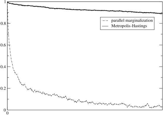
Figure 1: Autocorrelation of $Y^{n}_{mid}$ for Metropolis-Hastings method with 1-d Gaussian random walk proposals (solid) and parallel marginalization (dotted). The x-axis runs from 0 to 10000 iterations of the Metropolis-Hastings method and from 0 to 1000 iterations of parallel marginalization. This rescaling more than compensates for the extra work for parallel marginalization per iteration.

In these numerical examples, parallel marginalization is applied with a slight simplification as detailed in the following algorithm.

Algorithm 3.

The chain moves from $Y^{n}$ to $Y^{n+1}$ as follows:

1. Generate M independent Gaussian random paths $\left\{\zeta^{m}\left(n\right)\right\}_{n\in\widetilde{S}_{l}}$ with independent components $\zeta^{m}\left(n\right)$ of mean 0 and variance $2^{l-1}\triangle$.

2. For each $j$ and $n\in\widetilde{S}_{l}$ let

   $$U^{m}\left(n\right)=\zeta^{m}\left(n\right)+0.5\left(x_{l+1}(n-1)+x_{l+1}(n+1)\right).$$

3. Define the weights

   $$W_{U}^{m}=\frac{\pi_{l}\left(x_{l+1},U^{m}\right)}{p_{l}\left(U^{m}|x_{l+1}\right)},$$

   where $p_{l}$ is defined by the choice in step 1 as

   $$p_{l}\left(\tilde{x}_{l}|\hat{x}_{l}\right)\propto\exp\left(\sum_{n\in\widetilde{S}_{l}}-\frac{\left(\tilde{x}_{l}(n)-0.5\left(\hat{x}_{l}(n-1)+\hat{x}_{l}(n+1)\right)\right)^{2}}{2^{l}\triangle}\right).$$

4. Choose $J\in\left\{1,\dots,M\right\}$ according to the probabilities

   $$\mathbf{P}\left[J=j\right]=\frac{W_{U}^{j}}{\sum_{k=1}^{M}W_{U}^{k}}.$$

   Set $\widetilde{Y}^{\prime}=U^{J}.$

5. Set $V^{J}=\tilde{x}_{l}$ and for $j\neq J$ set

   $$V^{j}\left(n\right)=\zeta^{j}\left(n\right)+0.5\left(\hat{x}_{l}(n-1)+\hat{x}_{l}(n+1)\right).$$

6. Define the weights

   $$W_{V}^{m}=\frac{\pi_{l}\left(\hat{x}_{l},V^{m}\right)}{p_{l}\left(V^{m}|\hat{x}_{l}\right)}.$$

7. Set

   $$Y^{n+1}=\left(\dots,x_{l+1},\tilde{y}_{l},\hat{x}_{l},\dots\right)$$

   with probability

   $$A^{M}_{l}=\min\biggl{\{}1,\ \frac{\pi_{l+1}(\hat{x}_{l})\sum_{m=1}^{M}W^{m}_{U}}{\pi_{l+1}(x_{l+1})\sum_{m=1}^{M}W^{m}_{V}}\biggr{\}}$$ (13)

   and

   $$Y^{n+1}=Y^{n}=\left(\dots,\hat{x}_{l},\tilde{x}_{l},x_{l+1},\dots\right)$$

   with probability $1-A^{M}_{l}$.

This simplification reduces by half the number of gaussian random variables needed to evaluate the acceptance probability but may not be appropriate in all settings. For this problem, the choice of $M$ in (13), the number of samples $U^{m}$ and $V^{m}$, seems to have little effect on the swap acceptance rates. In the numerical experiment $M=l+1$ for swaps between levels $l$ and $l+1$.

The results of the Metropols-Hastings and parallel marginalization methods applied to the above bridge sampling problem after a run time of 10 minutes on a standard workstation are presented in Figures 2 and 3. Apparently the sample generated by parallel marginalization is a reasonable bridgepath while the Metropolis-Hastings method has clearly not converged.

Figure 2: Metropolis generated bridge path from Section 3.1 after a 10 minute run on a standard desktop workstation. Clearly the method has not converged.

Figure 3: Parallel marginalization generated bridge path from Section 3.1 after a 10 minute run on a standard desktop workstation. Apparently the method has converged.

3.2 Non-linear smoothing/filtering

In the non-linear smoothing and filtering problem one seeks to approximate conditional expectations of the form

$$\mathbf{E}\left[g\left(Z(0),Z(t_{1}),\dots,Z(T)\right)\ |\left\{H(j)=h(j)\right\}_{0}^{K}\right]$$

where the real valued processes $Z(t)$ and $H(j)$ are given by the system

$$\begin{split}&dZ(t)=f\left(Z(t)\right)dt+\sigma\left(Z(t)\right)dW(t),\\ &H(j)=r\left(Z(s_{j})\right)+\chi(j),\\ &Z(0)\sim\rho,\ \ \ \ \chi(j)\sim i.i.d.\ \mu.\end{split}$$ (14)

$g$, $f$, $\sigma$, and $r$ are real valued functions of $\mathbb{R}$. The $\chi(j)$ are real valued independent random variable drawn from the density $\mu$ and are independent of the Brownian motion $W(t).$ $\left\{s_{j}\right\}\subset\left\{t_{j}\right\},$ and $0=s_{0}<s_{1}<...<s_{K}=T.$ The process $Z(t)$ is a hidden signal and the $H(j)$ are noisy observations. The idea of computing the above conditional expectation by conditional path sampling has been suggested in [18, 19]. Popular alternatives include particle filters (see [20]) and ensemble Kalman filters (see [21]).

Again, begin by discretizing the system. Assume that $N_{j}=N\left(s_{j+1}-s_{j}\right)-1$ is an integer and let $\triangle=\frac{T}{N}.$ The linearly implicit Euler scheme gives

$$\begin{split}&X(j,n+1)=X(j,n)+f\left(X(j,n)\right)\triangle\\ &\ \ \ \ +\left(X(j,n+1)-X(j,n)\right)f^{{}^{\prime}}\left(X(j,n)\right)\triangle+\sigma\left(X(j,n)\right)\sqrt{\triangle}\ \xi(j,n),\\ \ &H(j)=r\left(X(j)\right)+\chi(j),\\ &X(0)=Z(0)\ \ \ \ \chi(j)\sim i.i.d.\ \mu\end{split}$$

where $X(j,n)$ represents the discrete time approximation to $Z(s_{j}+n\triangle),$ for $0\leq n\leq N_{j}.$ The $\xi(n)$ are independent Gaussian random variables with mean 0 and variance 1. The $\xi(n)$ are independent of the $\chi^{m}$. $N$ is again assumed to be a power of 2.

The approximate path measure for this problem is

$$\pi_{0}\left(x_{0}(0),\dots,x_{0}(N)\ |h(0),\dots,h(K)\right)\\ \propto\exp\left(-\sum_{k=0}^{N-1}\mathcal{V}\left(x_{0}(n),x_{0}(n+1),\triangle\right)\right)\\ \times\rho\left(x_{0}(0)\right)\prod_{n=0}^{K}\mu\left(x_{0}(j)-r\left(h(j)\right)\right)$$

The approximate marginals are chosen as

$$\pi_{l}\left(\left\{x_{l}(n)\right\}_{n\in S_{l}}\ |h(0),\dots,h(K)\right)\propto\\ q_{l}\left(\left\{x_{l}(n)\right\}_{n\in S_{l}}\right)\rho\left(x_{l}(0)\right)\prod_{n=0}^{K}\mu\left(x_{l}(j)-r\left(h(j)\right)\right)$$

where $V$, $q_{l}$ and $S_{l}$ are as defined in the previous section.

In this example, samples of the smoothed path are generated between time time 0 and time 10 for the same diffusion in a double well potential. The densities $\mu$ and $\rho$ are chosen as

$$\mu=N(0,0.01)\ \ \text{and}\ \ \rho(x)\propto\exp\left(-\left(x^{2}-1\right)^{2}\right)$$

The function $r$ in (14) is the identity function. The observation times are $s_{0}=0,s_{1}=1,\dots,s_{10}=10$ with $H(j)=-1$ for $j=0,\dots,5$ and $H(j)=1$ for $j=6,\dots,10$. $\triangle=2^{-10}.$ There are 8 chains ($L=7$). The observed swap acceptance rates are reported in table (3.2). Notice that the swap rates are again highest at the lower levels but, for this problem, become unreasonably small at the highest level.

Swap acceptance rates for filtering/smoothing problems Levels¹ 0/1 1/2 2/3 3/4 4/5 5/6 6/7 0.86 0.83 0.74 0.65 0.46 0.23 0.04

• Swaps between levels $l$ and $l+1.$

Again, $Y^{n}_{mid}\in\mathbb{R}$ denotes the midpoint of the path defined by $Y^{n}_{0}$ (i.e. an approximate sample of the path at time 5). In Figure 4 the autocorrelation of $Y^{n}_{mid}$ is compared to that of a standard Metropolis-Hastings rule. The figure has been adjusted as in the previous example. The relaxation time of the parallel chain is again clearly reduced.

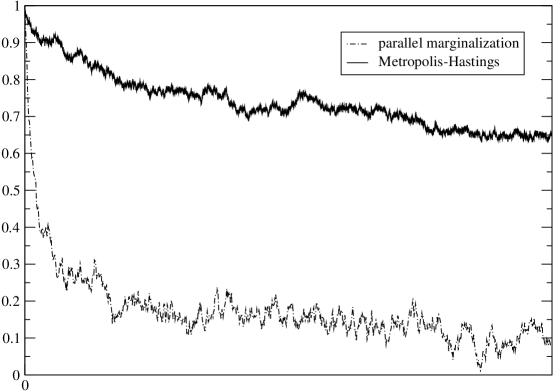
Figure 4: Autocorrelation of $Y^{n}_{mid}$ for Metropolis-Hastings method with 1-d Gaussian random walk proposals (solid) and parallel marginalization (dotted). The x-axis runs from 0 to 10000 iterations of the Metropolis-Hastings method and from 0 to 1000 iterations of parallel marginalization. This rescaling more than compensates for the extra work for parallel marginalization per iteration.

The algorithm is modified as in the previous example. For this problem, acceptable swap rates require a higher choice of $M$ in (13) than needed in the bridge sampling problem. In this numerical experiment $M=2^{l}$ for swaps between levels $l$ and $l+1$.

The results of the Metropols-Hastings and parallel marginalization methods applied to the smoothing problem above after a run time of 10 minutes on a standard workstation are presented in figure 5 and 6. Apparently the sample generated by parallel marginalization is a reasonable bridgepath while the Metropolis-Hastings method has clearly not converged.

Figure 5: Metropolis-Hastings generated smoothed path from Section 3.2 after a 10 minute run on a standard desktop workstation. Clearly the method has not converged.

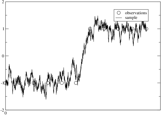
Figure 6: Parallel marginalization generated smoothed path from Section 3.2 after a 10 minute run on a standard desktop workstation. Apparently the method has converged.

4 Conclusion

A Markov chain Monte Carlo method has been proposed and applied to two conditional path sampling problems for stochastic differential equations. Numerical results indicate that this method, parallel marginalization, can have a dramatically reduced equilibration time when compared to standard MCMC methods.

Note that parallel marginalization should not be viewed as a stand alone method. Other acceleration techniques such as hybrid Monte Carlo can and should be implemented at each level within the parallel marginalization framework. As the smoothing problem indicates, the acceptance probabilities at coarser levels can become small. The remedy for this is the development of more accurate approximate marginal distributions by, for example, the methods in [6] and [8].

5 Acknowledgments

I would like to thank Prof. A. Chorin for his guidance during this research, which was carried out while I was a Ph.D. student at U. C. Berkeley. I would also like to thank Prof. O. Hald, Dr. P. Okunev, Dr. P. Stinis, and Dr. Xuemin Tu, for their very helpful comments. This work was supported by the Director, Office of Science, Office of Advanced Scientific Computing Research, of the U. S. Department of Energy under Contract No. DE-AC03-76SF00098 and National Science Foundation grant DMS0410110.

References

- [1] Leo P. Kadanoff. Statistical physics. World Scientific Publishing Co. Inc., River Edge, NJ, 2000. Statics, dynamics and renormalization.
- [2] J.J. Binney, N.J.Dowrick, A.J. Fisher, and M.E.J. Newman. The Theory of Critical Phenomena: An Introduction to the Renormalization Group. Oxford University Press, USA, 1992.
- [3] J. Goodman and A. Sokal. Multigrid Monte Carlo methods for lattice field theories. Phys. Rev. Lett., 56:1015–1018, 1986.
- [4] J. Goodman and A. Sokal. Multigrid Monte Carlo method: Conceptual foundations. Phys. Rev. D, 40(6):2035–2071, 1989.
- [5] A. Brandt and D. Ron. Renormalization multigrid (rmg): coarse-to-fine Monte Carlo acceleration and optimal derivation of macroscopic descriptions. J. Stat. Phys., 102(1/2):163–186, 2001.
- [6] Alexandre J. Chorin. Conditional expectations and renormalization. Multiscale Model. Simul., 1(1):105–118 (electronic), 2003.
- [7] Alexandre J. Chorin and Ole H. Hald. Stochastic tools in mathematics and science, volume 1 of Surveys and Tutorials in the Applied Mathematical Sciences. Springer, New York, 2006.
- [8] Panagiotis Stinis. A maximum likelihood algorithm for the estimation and renormalization of exponential densities. J. Comput. Phys., 208(2):691–703, 2005.
- [9] Pavel Okunev. Renormalization methods with applications to spin physics. U. C. Berkeley Math. Dept., 2005.
- [10] Alexandre J. Chorin. Monte Carlo without chains, with applications to spin glasses. in preparation.
- [11] Jonathan Weare. Efficient conditional path sampling of stochastic differential equations by parallel marginalization. submitted to Proc. Nat. Acad. Sci. USA.
- [12] Jun S. Liu. Monte Carlo Strategies in Scientific Computing. Springer, 2002.
- [13] Jun S. Liu, Faming Liang, and Wing Hung Wong. The multiple-try method and local optimization in metropolis sampling. J. Amer. Statist. Assoc., 95(449):121–134, 2000.
- [14] Z. Qin and J. S. Liu. Multi-point metropolis method with application to hybrid Monte Carlo. J. Comp. Phys., 172:827–840, 2001.
- [15] S. P. Meyn and R. L. Tweedie. Markov chains and stochastic stability. Communications and Control Engineering Series. Springer-Verlag London Ltd., London, 1993.
- [16] G. N. Milstein, E. Platen, and H. Schurz. Balanced implicit methods for stiff stochastic systems. SIAM J. Numer. Anal., 35(3):1010–1019 (electronic), 1998.
- [17] Peter E. Kloeden and Eckhard Platen. Numerical solution of stochastic differential equations, volume 23 of Applications of Mathematics (New York). Springer-Verlag, Berlin, 1992.
- [18] Francis Alexander, Greg Eyink, and Juan Restrepo. Accelerated Monte Carlo for optimal estimation of time series. J. Stat. Phys., 119:1331–1345, 2004.
- [19] Andrew M. Stuart, Jochen Voss, and Petter Wiberg. Fast communication conditional path sampling of SDEs and the Langevin MCMC method. Commun. Math. Sci., 2(4):685–697, 2004.
- [20] Nando De Freitas, Arnaud Doucet, and Neil Gordon. Sequential Monte Carlo Methods in Practice. Springer, 2005.
- [21] G. Evensen. The ensemble kalman filter: theoretical formulation and practical impementation. Ocean Dynamics, 53:343–367, 2003.