Tuning the stochastic background of gravitational waves with theory and observations

Abstract

In this this paper the stochastic background of gravitational waves (SBGWs) is analyzed with the auxilium of the WMAP data. We emphasize that, in general, in previous works in the literature about the SBGWs, old COBE data were used. After this, we want to face the problem of how the SBGWs and f(R) gravity can be related, showing, vice versa, that a revealed SBGWs could be a powerly probe for a given theory of gravity. In this way, it will also be shown that the conformal treatment of SBGWs can be used to parametrize in a natural way f(R) theories.

¹INFN - Sezione di Pisa and Università di Pisa, Via F. Buonarroti 2, I - 56127 PISA

²Dipartimento di Scienze Fisiche, Università di Napoli “Federico II”, INFN Sezione di Napoli, Compl. Univ di Monte S. Angelo, Edificio G, via Cinthia, I-80126, Napoli, Italy

³ Relativity and Gravitation Group Politecnico di Torino, Corso Duca degli Abruzzi 24, I - 10129 Torino, Italy

• PACS numbers: 04.80.Nn, 04.30.Nk, 04.50.+h

• Keywords: gravitational waves; extended theories of gravity; stochastic background;

1 Introduction

The accelerate expansion of the Universe, which is today observed, shows that cosmological dynamic is dominated by the so called Dark Energy which gives a large negative pressure. This is the standard picture, in which such new ingredient is considered as a source of the rhs of the field equations. It should be some form of un-clustered non-zero vacuum energy which, together with the clustered Dark Matter, drives the global dynamics. This is the so called “concordance model” (ACDM) which gives, in agreement with the CMBR, LSS and SNeIa data, a good trapestry of the today observed Universe, but presents several shortcomings as the well known “coincidence” and “cosmological constant” problems [1].

An alternative approach is changing the lhs of the field equations, seeing if observed cosmic dynamics can be achieved extending general relativity [2, 3, 4, 5]. In this different context, it is not required to find out candidates for Dark Energy and Dark Matter, that, till now, have not been found, but only the “observed” ingredients, which are curvature and baryonic matter, have to be taken into account. Considering this point of view, one can think that gravity is not scale-invariant [5] and a room for alternative theories is present [6, 7, 8]. In principle, the most popular Dark Energy and Dark Matter models can be achieved considering $f(R)$ theories of gravity [2, 3, 4], where $R$ is the Ricci curvature scalar. In this picture even the sensitive detectors for gravitational waves, like bars and interferometers (i.e. those which are currently in operation and the ones which are in a phase of planning and proposal stages) [9, 10, 11, 12, 13, 14, 15, 16], could, in principle, be important to confirm or ruling out the physical consistency of general relativity or of any other theory of gravitation. This is because, in the context of Extended Theories of Gravity, some differences between General Relativity and the others theories can be pointed out starting by the linearized theory of gravity [6, 17, 18, 19].

This philosophy can be taken into account also for the SBGWs which, together with cosmic microwave background radiation (CMBR), would carry, if detected, a huge amount of information on the early stages of the Universe evolution [2, 20, 21]). Also in this case, a key role for the production and the detection of this graviton background is played by the adopted theory of gravity [21].

In the second section of this paper the SBGWs is analyzed with the auxilium of the WMAP data [20, 22, 23]. We emphasize that, in general, in previous works in the literature about the SBGWs, old COBE data were used (see [24, 25, 26, 27, 28, 29] for example).

In the third section we want to face the problem of how the SBGWs and f(R) gravity can be related, showing, vice versa, that a revealed SBGWs could be a powerly probe for a given theory of gravity. In this way, it will also be shown that the conformal treatment of SBGWs can be used to parametrize in a natural way f(R) theories.

2 Tuning the stochastic background of gravitational waves using the WMAP data

From our analysis, it will result that the WMAP bounds on the energy spectrum and on the characteristic amplitude of the SBGWs are greater than the COBE ones, but they are also far below frequencies of the earth-based antennas band. At the end of this section a lower bound for the integration time of a potential detection with advanced LIGO is released and compared with the previous one arising from the old COBE data. Even if the new lower bound is minor than the previous one, it results very long, thus for a possible detection we hope in the LISA interferometer and in a further growth in the sensitivity of advanced projects.

The strongest constraint on the spectrum of the relic SBGWs in the frequency range of ground based antennas like bars and interferometers, which is the range $10Hz\leq f\leq 10^{4}Hz$, comes from the high isotropy observed in the CMBR.

The fluctuation $\Delta T$ of the temperature of CBR from its mean value $T_{0}=2.728$ K varies from point to point in the sky [20, 22, 23], and, since the sky can be considered the surface of a sphere, the fitting of $\Delta T$ is performed in terms of a Laplace series of spherical harmonics

$$\frac{\Delta T}{T_{0}}(\hat{\Omega})=\sum_{l=1}^{\infty}\sum_{m=-l}^{l}a_{lm}Y_{lm}(\hat{\Omega}),$$ (1)

and the fluctations are assumed statistically independent ($<a_{lm}>=0$, $<a_{lm}a_{l^{\prime}m^{\prime}}^{*}>=C_{l}\delta_{ll^{\prime}}\delta_{mm^{\prime}}$). In eq. (1) $\hat{\Omega}$ denotes a point on the 2-sphere while the $a_{lm}$ are the multipole moments of the CMBR. For details about the definition of statistically independent fluctations in the context of the temperature fluctations of CMBR see [24, 25].

The WMAP data [22, 23] permit a more precise determination of the rms quadrupole moment of the fluctations than the COBE data

$$Q_{rms}\equiv T(\sum_{m=-2}^{2}\frac{|a_{2m}|^{2}}{4\pi})^{\frac{1}{2}}=8\pm 2\mu K,$$ (2)

while in the COBE data we had [25, 26, 27]

$$Q_{rms}=14.3_{-3.3}^{+5.2}\mu K.$$ (3)

A connection between the fluctuation of the temperature of the CMBR and the SBGWs derives from the Sachs-Wolfe effect [20, 30]. Sachs and Wolfe showed that variations in the density of cosmological fluid and GWs perturbations result in the fluctuation of the temperature of the CMBR, even if the surface of last scattering had a perfectly uniform temperature [30]. In particular the fluctuation of the temperature (at the lowest order) in a particular point of the space is

$$\frac{\Delta T}{T_{0}}(\hat{\Omega})=\frac{1}{2}\int_{nullgeodesic}d\lambda\frac{\partial}{\partial\eta}h_{rr}.$$ (4)

The integral in eq. (4) is taken over a path of null geodesic which leaves the current spacetime point heading off in the direction defined by the unit vector $\hat{\Omega}$ and going back to the surface of last scattering of the CMBR.

Here $\lambda$ is a particular choice of the affine parameter along the null geodesic. By using conformal coordinates, we have for the metric perturbation

$$\delta g_{ab}=R^{2}(\eta)h_{ab},$$ (5)

and $r$ in eq. (4) is a radial spatial coordinate which goes outwards from the current spacetime point. The effect of a long wavelenght GW is to shift the temperature distribution of CMBR from perfect isotropy. Because the fluctations are very small ($<\Delta T/T_{0}>\leq 5*10^{-5}$ [22, 23]), the perturbations caused by the relic SBGWs cannot be too large.

The WMAP results give rather tigh constraints on the spectrum of the SBGWs at very long wavelenghts. In [24, 25] we find a constraint on $\Omega_{gw}(f)$ which derives from the COBE observational limits, given by

$$\Omega_{gw}(f)h_{100}^{2}<7*10^{-11}(\frac{H_{0}}{f})^{2}\textrm{ for }H_{0}<f<30H_{0}.$$ (6)

Now the same constraint will be obtained from the WMAP data [20]. Because of its specific polarization properties, relic SBGWs should generate particular polarization pattern of CMBR anisotropies, but the detection of CMBR polarizations is not fulfiled today [31]. Thus an indirect method will be used. We know that relic GWs have very long wavelenghts of Hubble radius size, so the CMBR power spectrum from them should manifest fast decrease at smaller scales (hight multipole moments). But we also know that scalar modes produce a rich CMBR power spectrum at large multipole moments (series of acoustic peaks, ref. [22, 23]). Then the properties of tensor modes of cosmological perturbations of spacetime metric can be extract from observational data using angular CMBR power spectrum combined with large scale structure of the Universe. One can see (fig. 1 ) that in the range $2\leq l\leq 30$ (the same used in [25], but with the old COBE data [32]) scalar and tensor contributions are comparable. From [22, 23], the WMAP data give for the tensor/scala ratio $r$ the constraint $r<0.9$. ($r<0.5$ in the COBE data, ref. [32]); Novosyadly and Apunevych obtained $\Omega_{scalar}(H_{0})<2.7*10^{-9}$ [31]. Thus, if one remembers that, at order of Hubble radius, the tensorial spectral index is $-4\leq n_{t}\leq-2$ [20], it results

$$\Omega_{gw}(f)h_{100}^{2}<1.6*10^{-9}(\frac{H_{0}}{f})^{2}\textrm{ for }H_{0}<f<30H_{0},$$ (7)

which is greater than the COBE data result of eq. (6).

We emphasize that the limit of eq. (7) is not a limit for any GWs, but only for relic ones of cosmological origin, which were present at the era of the CMBR decoupling. Also, the same limit only applies over very long wavelenghts (i.e. very low frequencies) and it is far below frequencies of the Virgo - LIGO band.

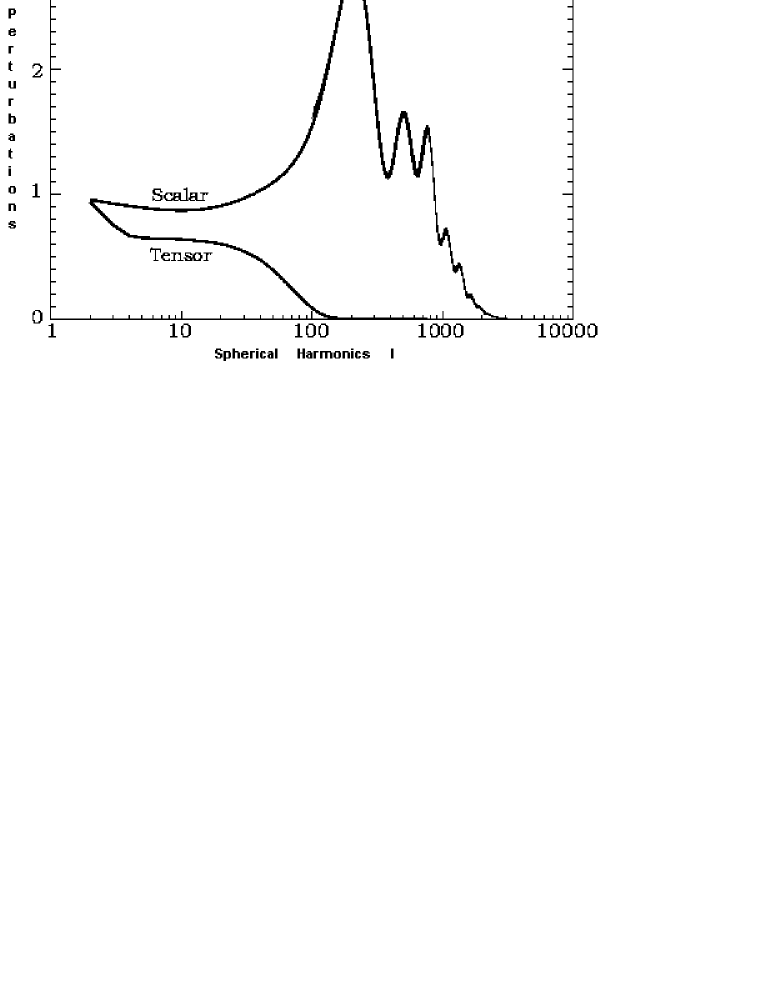
Figure 1: The tensor to scalar ratio

The primordial production of the relic SBGWs has been analyzed in [25, 26, 27, 33] (note: a generalization for f(R) theories of gravity will be given in the next section following [21]), where it has been shown that in the range $10^{-15}Hz\leq f\leq 10^{10}Hz$ the spectrum is flat and proportional to the ratio

$$\frac{\rho_{ds}}{\rho_{Planck}}\approx 10^{-12}.$$ (8)

WMAP observations put strongly severe restrictions on the spectrum, as we discussed above. In fig. 2 the spectrum $\Omega_{gw}$ is mapped: the amplitude (determined by the ratio $\frac{\rho_{ds}}{\rho_{Planck}}$) has been chosen to be as large as possible, consistent with the WMAP constraint (7).

Figure 2: The spectrum of relic gravitons in inflationary models is flat over a wide range of frequencies. The horizontal axis is $\log_{10}$ of frequency, in Hz. The vertical axis is $\log_{10}\Omega_{gr}$. The inflationary spectrum rises quickly at low frequencies (wave which rentered in the Hubble sphere after the Universe became matter dominated) and falls off above the (appropriately redshifted) frequency scale $f_{max}$ associated with the fastest characteristic time of the phase transition at the end of inflation. The amplitude of the flat region depends only on the energy density during the inflationary stage; we have chosen the largest amplitude consistent with the WMAP constrain discussed earlier: $\Omega_{gr}(f)h_{100}^{2}<1.6*10^{-9}$ at $10^{-18}Hz$. This means that at Virgo and Lisa frequencies, $\Omega_{gr}(f)h_{100}^{2}<9*10^{-13}$

Nevertheless, because the spectrum falls off $\propto f^{-2}$ at low frequencies [25, 26, 27, 33], this means that today, at Virgo and LISA frequencies, indicated in fig. 2,

$$\Omega_{gw}(f)h_{100}^{2}<9*10^{-13},$$ (9)

while using the COBE data it was

$\Omega_{gw}(f)h_{100}^{2}<8*10^{-14}$(refs. [25, 32]).

It is interesting to calculate the correspondent strain at $\approx 100Hz$, where interferometers like Virgo and LIGO have a maximum in sensitivity. The well known equation for the characteristic amplitude [20, 24, 25, 29] can be used:

$$h_{c}(f)\simeq 1.26*10^{-18}(\frac{1Hz}{f})\sqrt{h_{100}^{2}\Omega_{gw}(f)},$$ (10)

obtaining

$$h_{c}(100Hz)<1.7*10^{-26}.$$ (11)

Then, because for ground-based interferometers a sensitivity of the order of $10^{-22}$ is expected at $\approx 100Hz$, four order of magnitude have to be gained in the signal to noise ratio [9, 10, 11, 12, 13, 14, 15, 16]. Let us analyze smaller frequencies too. The sensitivity of the Virgo interferometer is of the order of $10^{-21}$ at $\approx 10Hz$ [9, 10] and in that case it is

$$h_{c}(10Hz)<1.7*10^{-25}.$$ (12)

For a better understanding of the difficulties on the detection of the SBGWs a lower bound for the integration time of a potential detection with advanced LIGO is released. For a cross-correlation between two interferometers the signal to noise ratio (SNR) increases as

$$(SNR)=\sqrt{2T}\frac{H_{0}^{2}}{5\pi^{2}}\sqrt{\int_{0}^{\infty}df\frac{\Omega_{gw}^{2}(f)\gamma^{2}(f)}{f^{6}P_{1}(|f|)P_{2}(|f|)}}.$$ (13)

where $P_{i}(|f|)$ is the one-sided power spectral density of the $i$ detector [34] and $\gamma(f)$ the well known overlap-reduction function [34, 35]. Assuming two coincident coaligned detectors $(\gamma(f)=1)$ with a noise of order $10^{-48}/Hz$ (i.e. a typical value for the advanced LIGO sensitivity [36]) one gets $(SNR)\sim 1$ for $\sim 3*10^{5}years$ using our result $\Omega_{gw}(f)h_{100}^{2}\sim 9*10^{-13}$ while it is $(SNR)\sim 1$ for $\sim 3*10^{7}years$ using previous COBE result $\Omega_{gw}(f)h_{100}^{2}\sim 8*10^{-14}$. Since the overlap reduction function degrades the SNR, these results can be considered a solid upper limit for the advanced LIGO configuration for the two different values of the spectrum.

The sensitivity of the LISA interferometer will be of the order of $10^{-22}$ at $10^{-3}Hz$ [37] and in that case it is

$$h_{c}(10^{-3}Hz)<1.7*10^{-21}.$$ (14)

Then a stochastic background of relic gravitational waves could be in principle detected by the LISA interferometer. We also hope in a further growth in the sensitivity of advanced projects.

We emphasize that the assumption that all the tensorial perturbation in the Universe are due to a SBGWs is quit strong, but our results (9), (11), (12) and (14) can be considered like upper bounds.

Reasuming, in this section the SBGWs has been analyzed with the auxilium of the WMAP data, while previous works in literature, used the old COBE data, seeing that the predicted signal for these relic GWs is very weak. From our analysis it resulted that the WMAP bound on the energy spectrum and on the characteristic amplitude of the SBGWs are greater than the COBE ones, but they are also far below frequencies of the earth-based antennas band. In fact the integration time of a potential detection with advanced interferometers is very long, thus, for a possible detection we have to hope in a further growth in the sensitivity of advanced ground based projects and in the LISA interferometer.

3 Tuning the stochastic background of gravitational waves with f(R) theories of gravity

GWs are the perturbations $h_{\alpha\beta}$ of the metric $g_{\alpha\beta}$ which transform as three-tensors. Following [21, 38], the GW-equations in the TT gauge are

$$\square h_{i}^{j}=0,$$ (15)

where $\square\equiv(-g)^{-1/2}\partial_{\alpha}(-g)^{1/2}g^{\alpha\beta}\partial_{\beta}$ is the usual d’Alembert operator and these equations are derived from the Einstein field equations deduced from the Hilbert Lagrangian density $L=R$ [6, 21]. Clearly, matter perturbations do not appear in (15) since scalar and tensor perturbations do not couple with tensor perturbations in Einstein equations. The Latin indices run from 1 to 3, the Greek ones from 0 to 3. Our task is now to derive the analog of eqs. (15) assuming a generic theory of gravity given by the action

$$A=\frac{1}{2k}\int d^{4}x\sqrt{-g}f(R),$$ (16)

where, for a sake of simplicity, we have discarded matter contributions. A conformal analysis will help in this goal. In fact, assuming the conformal transformation

$$\tilde{g}_{\alpha\beta}=e^{2\Phi}g_{\alpha\beta}$$ (17)

where the conformal rescaling

$$e^{2\Phi}=f^{\prime}(R)$$ (18)

has been chosen being the prime the derivative with respect to the Ricci curvature scalar and $\Phi$ the “conformal scalar field”, we obtain the conformally equivalent Hilbert-Einstein action

$$A=\frac{1}{2k}\int d^{4}x\sqrt{-\widetilde{g}}[\widetilde{R}+L(\Phi,\Phi_{;\alpha})],$$ (19)

where $L(\Phi,\Phi_{;\alpha})$ is the conformal scalar field contribution derived from

$$\tilde{R}_{\alpha\beta}=R_{\alpha\beta}+2(\Phi_{;\alpha}\Phi_{;\beta}-g_{\alpha\beta}\Phi_{;\delta}\Phi^{;\delta}-\frac{1}{2}g_{\alpha\beta}\Phi^{;\delta}{}_{;\delta})$$ (20)

and

$$\tilde{R}=e^{-2\Phi}+(R-6[]\Phi-6\Phi_{;\delta}\Phi^{;\delta}).$$ (21)

In any case, as we will see, the $L(\Phi,\Phi_{;\alpha})$-term does not affect the GWs-tensor equations so it will not be considered any longer (note: a scalar component in GWs is often considered [17, 39, 40, 41], but here we are taking into account only the genuine tensor part of stochastic background).

Starting from the action (19) and deriving the Einstein-like conformal equations, the GWs equations are

$$\widetilde{\square}\widetilde{h}_{i}^{j}=0,$$ (22)

expressed in the conformal metric $\tilde{g}_{\alpha\beta}.$ Since no scalar perturbation couples to the tensor part of gravitational waves it is

$$\widetilde{h}_{i}^{j}=\widetilde{g}^{lj}\delta\widetilde{g}_{il}=e^{-2\Phi}g^{lj}e^{2\Phi}\delta g_{il}=h_{i}^{j},$$ (23)

which means that $h_{i}^{j}$ is a conformal invariant.

As a consequence, the plane wave amplitude $h_{i}^{j}=h(t)e_{i}^{j}\exp(ik_{i}x^{j}),$ where $e_{i}^{j}$ is the polarization tensor, are the same in both metrics. In any case the d’Alembert operator transforms as

$$\widetilde{\square}=e^{-2\Phi}(\square+2\Phi^{;\alpha}\partial_{;\alpha})$$ (24)

and this means that the background is changing while the tensor wave amplitude is fixed.

In order to study the cosmological stochastic background, the operator (24) can be specified for a Friedman-Robertson-Walker metric [26, 27], and the equation (22) becomes

$$\ddot{h}+(3H+2\frac{d\Phi}{dt})\frac{dh}{dt}+k^{2}a^{-2}h=0,$$ (25)

being $\square=\frac{\partial}{\partial t^{2}}+3H\frac{\partial}{\partial t}$, $a(t)$ the scale factor and $k$ the wave number. It has to be emphasized that equation (25) applies to any f(R) theory whose conformal transformation can be defined as $e^{2\Phi}=f^{\prime}(R).$ The solution, i.e. the GW amplitude, depends on the specific cosmological background (i.e. $a(t)$) and the secific theory of gravity (i.e. $\Phi(t)$). For example, assuming power law behaviors for $a(t)$ and $\Phi(t)=\frac{1}{2}\ln f^{\prime}(R(t)),$ that is

$$\Phi(t)=f^{\prime}(R)=f_{0}^{\prime}(\frac{t}{t_{0}})^{m},\textrm{ $$$$$$$$$$$$$$$$ }a(t)=a_{0}(\frac{t}{t_{0}})^{n},$$ (26)

it is easy to show that general relativity is recovered for $m=0$ while

$$n=\frac{m^{2}+m-2}{m+2}$$ (27)

is the relation between the parameters for a generic $f(R)=f_{0}R^{s}$ where $s=1-\frac{m}{2}$ with $s\models 1$ [42]. Equation (25) can be recast in the form

$$\ddot{h}+(3n+m)t^{-1}\frac{dh}{dt}+k^{2}a_{0}(\frac{t_{0}}{t})^{2n}h=0,$$ (28)

whose general solution is

$$h(t)=(\frac{t_{0}}{t})^{-\beta}[C_{1}J_{\alpha}(x)+C_{2}J_{-\alpha}(x)].$$ (29)

$J_{\alpha}$’s are Bessel functions and

$$\alpha=\frac{1-3n-m}{2(n-1)},\textrm{ $$$$$$}\beta=\frac{1-3n-m}{2},\textrm{ $$$$$$}x=\frac{kt^{1-n}}{1-n}$$ (30)

while $t_{0},$ $C_{1},$ and $C_{2}$ are constans related to the specific values of $n$ and $m.$

The time units are in terms of the Hubble radius $H^{-1};$ $n=1/2$ is a radiation-like evolution; $n=2/3$ is a dust-like evolution, $n=2$ labels power-law inflationary phases and $n=-5$ is a pole-like inflation. From eq. (27), a singular case is for $m=-2$ and $s=2.$ It is clear that the conformally invariant plane-wave amplitude evolution of the tensor GW strictly depends on the background.

Let us now take into account the iusse of the production of relic GWs contributing to the stochastic background. Several mechanisms can be considered as cosmological populations of astrophysical sources [43], vacuum fluctuations, phase transitions [24] and so on. In principle, we could seek for contributions due to every high-energy physical process in the early phases of the Universe evolution.

It is important to distinguish processes coming from transitions like inflation, where the Hubble flow emerges in the radiation dominated phase and process, like the early star formation rates, where the production takes place during the dust dominated era. In the first case, stochastic GWs background is strictly related to the cosmological model. This is the case we are considering here which is, furthermore, also connected to the specific theory of gravity. In particular, one can assume that the main contribution to the stochastic background comes from the amplification of vacuum fluctuactons at the transition between an inflationary phase and the radiation-dominated era. However, in any inflationary model, we can assume that the relic GWs generated as zero-point fluctuactions during the inflation undergoes adiabatically damped oscillations ($\sim 1/a$) until they reach the Hubble radius $H^{-1}.$ This is the particle horizon for the growth of perturbations. On the other hand, any other previous fluctuation is smoothed away by the inflationary expansion. The GWs freeze out for $a/k\gg H^{-1}$ and re-enter the $H^{-1}$ radius after the reheating in the Friedman era [21, 25, 26, 27, 33]. The re-enter in the radiation dominated or in the dust-dominated era depends on the scale of the GW. After the re-enter, GWs can be detected by their Sachs-Wolfe effect on the temperature anisotropy $\frac{\bigtriangleup T}{T}$ at the decoupling [30]. When $\Phi$ acts as the inflaton [21, 44] we have $\frac{d\Phi}{dt}\ll H$ during the inflation. Considering also the conformal time $d\eta=dt/a$, eq. (25) reads

$$h^{\prime\prime}+2\frac{\gamma^{\prime}}{\gamma}h^{\prime}+k^{2}h=0,$$ (31)

where $\gamma=ae^{\Phi}$and derivation is with respect to $\eta.$ Inflation means that $a(t)=a_{0}\exp(Ht)$ and then $\eta=\int dt/a=1/(aH)$ and $\frac{\gamma^{\prime}}{\gamma}=-\frac{1}{\eta}.$ The exact solution of (31) is

$$h(\eta)=k{}^{-3/2}\sqrt{2/k}[C_{1}(\sin k\eta-\cos k\eta)+C_{2}(\sin k\eta+\cos k\eta)].$$ (32)

Inside the $1/H$ radius it is $k\eta\gg 1.$ Furthermore considering the absence of gravitons in the initial vacuum state, we have only negative-frequency modes and then the adiabatic behavior is

$$h=k{}^{1/2}\sqrt{2/\pi}\frac{1}{aH}C\exp(-ik\eta).$$ (33)

At the first horizon crossing ($aH=k$), the averaged amplitude $A_{h}=(k/2\pi)^{3/2}|h|$ of the perturbations is

$$A_{h}=\frac{1}{2\pi{}^{2}}C$$ (34)

when the scale $a/k$ grows larger than the Hubble radius $1/H,$ the growing mode of evolution is constant, that it is frozen. This situation corresponds to the limit $-k\eta\ll 1$ in equation (32). Since $\Phi$ acts as the inflaton field, it is $\Phi\sim 0$ at re-enter (after the end of inflation). Then the amplitude $A_{h}$ of the wave is preserved until the second horizon crossing after which it can be observed, in principle, as an anisotropy perturbation of the CBR. It can be shown that $\frac{\bigtriangleup T}{T}\lesssim A_{h}$ is an upper limit to $A_{h}$ since other effects can contribute to the background anisotropy [45]. From this consideration, it is clear that the only relevant quantity is the initial amplitude $C$ in equation (33) which is conserved until the re-enter. Such an amplitude directly depends on the fundamental mechanism generating perturbations. Inflation gives rise to processes capable of producing perturbations as zero-point energy fluctations. Such a mechanism depends on the adopted theory of gravitation and then $\frac{\bigtriangleup T}{T}$ could constitute a further constraint to select a suitable f(R)-theory. Considering a single graviton in the form of a monocromatic wave, its zero-point amplitude is derived through the commutation relations

$$[h(t,x),\pi_{h}(t,y)]=i\delta^{3}(x-y)$$ (35)

calculated at a fixed time $t,$ where the amplitude $h$ is the field and $\pi_{h}$ is the conjugate momentum operator. Writing the lagrangian for $h$

$$\widetilde{L}=\frac{1}{2}\sqrt{\widetilde{g}}\widetilde{g}^{\alpha\beta}h_{;\alpha}h_{;\beta}$$ (36)

in the conformal FRW metric $\widetilde{g}_{\alpha\beta}$ ($h$ si conformally invariant), we obtain

$$\pi_{h}=\frac{\partial\widetilde{L}}{\partial(dh/dt)}=e^{2\Phi}a^{3}\frac{dh}{dt}.$$ (37)

Equation (35) becomes

$$[h(t,x),\frac{dh}{dt}(y,y)]=i\frac{\delta^{3}(x-y)}{e^{2\Phi}a^{3}}$$ (38)

and the fields $h$ and $\frac{dh}{dt}$ can be expanded in terms of creation and annihilation operators

$$h(t,x)=\frac{1}{(2\pi)^{3/2}}\int d^{3}k[h(t)e^{-ikx}+h^{*}(t)e^{ikx}]$$ (39)

$$\frac{dh}{dt}(t,x)=\frac{1}{(2\pi)^{3/2}}\int d^{3}k[\frac{dh}{dt}(t)e^{-ikx}+\frac{dh}{dt}^{*}(t)e^{ikx}].$$ (40)

The commutation relations in conformal time are then

$$[h(h^{\prime*}-h^{*}h^{\prime}]=i\frac{(2\pi)^{3}}{e^{2\Phi}a^{3}}.$$ (41)

Insering (33) and (34), we obtain $C=\sqrt{2}\pi{}^{2}He^{-\Phi}$ where $H$ and $\Phi$ are calculated at the first horizon crossing and then

$$A_{h}=\frac{\sqrt{2}}{2}{}He^{-\Phi},$$ (42)

which means that the amplitude of GWs produced during inflation directly depends on the given f(R) theory being $\Phi=\frac{1}{2}\ln f^{\prime}(R).$ Explicitly, it is

$$A_{h}=\frac{H}{\sqrt{2f^{\prime}(R)}}.$$ (43)

This result deserves some discussion and can be read in two ways. From one side the amplitude of relic GWs produced during inflation depends on the given theory of gravity that, if different from general relativity, gives extra degrees of freedom which assume the role of inflaton field in the cosmological dynamics [44]. On the other hand, the Sachs-Wolfe effect related to the CMBR temperatue anisotropy could constitute a powerful tool to test the true theory of gravity at early epochs, i.e. at very high redshift. This probe, related with data a medium [46] and low redshift [47], could strongly contribute

1. to reconstruct cosmological dynamics at every scale;

2. to further test general relativity or to rule out it against alternative theories;

3. to give constrains on the SBGWs, if f(R) theories ares independently probed at other scales.

Reasuming, in this section it has been shown that amplitudes of tensor GWs are conformally invariant and their evolution depends ond the cosmological SBGWs. Such a background is tuned by conformal scalar field which is not present in the standard general relativity. Assuming that primordial vacuum fluctuations produce a SBGWs, beside scalar perturbations, kinematical distorsions and so on, the initial amplitude of these ones is function of the f(R)-theory of gravity and then the SBGWs can be, in a certain sense, “tuned” by the theory. Vice versa, data coming fro the Sachs-Wolfe effect could contribute to select a suitable f(R)-theory which can be consistently matched with other observations. However, further and accurate studies are needed in order to test the relation between Sachs-Wolfe effect and f(R) gravity. This goal could be achieved in the next future through the forthcoming space (LISA) and ground based (Virgo, LIGO) interferometers.

4 Conclusions

The SBGWs has been analyzed with the auxilium of the WMAP data while, in general, in previous works in the literature about the SBGWs, old COBE data were used. After this, it has been shown how the SBGWs and f(R) gravity can be related, showing, vice versa, that a revealed SBGWs could be a powerly probe for a given theory of gravity. In this way, it has also been shown that the conformal treatment of SBGWs can be used to parametrize in a natural way f(R) theories.

References

- [1] Peebles PJE and Ratra B - Rev. Mod. Phys. 75 8559 (2003)
- [2] Allemandi G, Capone M, Capozziello S and Francaviglia M - Gen. Rev. Grav. 38 1 (2006)
- [3] Allemandi G, Francaviglia M, Ruggiero ML and Tartaglia A - Gen. Rel. Grav. 37 11 (2005)
- [4] Capozziello S - Int. J. Mod. Phys. D 11 483 (2002);
- [5] Capozziello S, Cardone VF and Troisi A - J. Cosmol. Astropart. Phys. JCAP08001 (2006)
- [6] Capozziello S - Newtonian Limit of Extended Theories of Gravity in Quantum Gravity Research Trends Ed. A. Reimer, pp. 227-276 Nova Science Publishers Inc., NY (2005) - also in arXiv:gr-qc/0412088 (2004)
- [7] Capozziello S and Troisi A - Phys. Rev. D 72 044022 (2005)
- [8] Will C M Theory and Experiments in Gravitational Physics, Cambridge Univ. Press Cambridge (1993)
- [9] Acernese F et al. (the Virgo Collaboration) - Class. Quant. Grav. 23 8 S63-S69 (2006)
- [10] Corda C - Astropart. Phys. 27, No 6, 539-549 (2007)
- [11] Hild S (for the LIGO Scientific Collaboration) - Class. Quant. Grav. 23 19 S643-S651 (2006)
- [12] Willke B et al. - Class. Quant. Grav. 23 8S207-S214 (2006)
- [13] Sigg D (for the LIGO Scientific Collaboration) - www.ligo.org/pdf_public/P050036.pdf
- [14] Abbott B et al. (the LIGO Scientific Collaboration) - Phys. Rev. D 72, 042002 (2005)
- [15] Ando M and the TAMA Collaboration - Class. Quant. Grav. 19 7 1615-1621 (2002)
- [16] Tatsumi D, Tsunesada Y and the TAMA Collaboration - Class. Quant. Grav. 21 5 S451-S456 (2004)
- [17] Capozziello S and Corda C - Int. J. Mod. Phys. D 15 1119 -1150 (2006); Corda C - Response of laser interferometers to scalar gravitational waves- talk in the Gravitational Waves Data Analysis Workshop in the General Relativity Trimester of the Institut Henri Poincare - Paris 13-17 November 2006, on the web in www.luth2.obspm.fr/IHP06/workshops/gwdata/corda.pdf
- [18] Corda C - J. Cosmol. Astropart. Phys. JCAP04009 (2007)
- [19] Corda C - Astropart. Phys. 28, 247-250 (2007)
- [20] Corda C - Mod. Phys. Lett. A 22, 16, 1167-1173 (2007)
- [21] Capozziello S, Corda C and De Laurentis MF - Mod. Phys. Lett. A 22, 15, 1097-1104 (2007)
- [22] C. L. Bennet and others - ApJS 148 1 (2003)
- [23] D. N. Spergel and others - ApJS 148 195 (2003)
- [24] Maggiore M- Physics Reports 331, 283-367 (2000)
- [25] B. Allen - Proceedings of the Les Houches School on Astrophysical Sources of Gravitational Waves, eds. Jean-Alain Marck and Jean-Pierre Lasota (Cambridge University Press, Cambridge, England 1998).
- [26] L. P. Grishchuk and others - Phys. Usp. 44 1-51 (2001)
- [27] L. P. Grishchuk and others - Usp. Fiz. Nauk 171 3 (2001)
- [28] Babusci D, Foffa F, Losurdo G, Maggiore M, Mattone G and Sturani R - Virgo DAD - www.virgo.infn.it/Documents/DAD/stochastic background
- [29] Corda C - Virgo Report: VIRGO-NOTE-PIS 1390-237 (2003) - www.virgo.infn.it/Documents
- [30] R. K. Sachs and A. M. Wolfe - ApJ 147, 73 (1967)
- [31] B. Novosyadlyj and S. Apunevych - proceedings of international confernce “Astronomy in Ukraine - Past, Present, Future” - Main Astronomical Observatory (2004)
- [32] J. P. Zibin, D. Scott and M. White - arXiv:astro-ph/9904228
- [33] B. Allen - Phys. Rev. D 37, 2078 (1988)
- [34] B. Allen and J. P. Romano - Phys. Rev. D 59 102001 (1999)
- [35] E. E. Flanagan - Phys. Rev. D 48 2389 (1993)
- [36] K. G. Arun, B. R. Iver, B. S. Sathyaprakash, and P. A. Sundararajan - Phys. Rev. D 71 084008 (2005)
- [37] www.lisa.nasa.org; www.lisa-scienze.org
- [38] S. Weimberg - Gravitation and Cosmology (Wiley 1972)
- [39] Maggiore M and Nicolis A - Phys. Rev. D 62 024004 (2000)
- [40] Tobar ME, Suzuki T and Kuroda K Phys. Rev. D 59 102002 (1999)
- [41] Corda C - Mod. Phys. Lett. A 22, No. 23, 1727-1735 (2007)
- [42] Capozziello S, Cardone VF, Carloni S and Troisi A - Int. J. Mod. Phys. D 12 1969 (2003)
- [43] Chiba T, Smith TL and Erickcek L - astro-ph/0611867 (2006)
- [44] Starobinsky AA - Phys. Lett. B 91, 99 (1980)
- [45] Starobinsky AA - Sov. Phys. JEPT Lett. B 34, 438 (1982)
- [46] Capozziello S, Cardone VF and Troisi A - Phys. Rev. D 71 0843503 (2005)
- [47] Capozziello S, Cardone VF , Funaro M and Andreon S - Phys. Rev. D 70 123501 (2004)