FADE, an instrument to measure the atmospheric coherence time

Abstract

Aims. After proposing a new method of deriving the atmospheric time constant from the speed of focus variations (Kellerer & Tokovinin 2007), we now implement it with the new instrument, FADE.

Methods. FADE uses a 36-cm Celestron telescope that is modified to transform stellar point images into a ring by increasing the central obstruction and combining defocus with spherical aberration. Sequences of images recorded with a fast CCD detector are processed to determine the defocus and its variations in time from the ring radii. The temporal structure function of the defocus is fitted with a model to derive the atmospheric seeing and time constant. We investigated by numerical simulation the data reduction algorithm and instrumental biases. Bias caused by instrumental effects, such as optical aberrations, detector noise, acquisition frequency, etc., is quantified. The ring image must be well-focused, i.e. must have a sufficiently sharp radial profile, otherwise, scintillation seriously affects the results. An acquisition frequency of 700 Hz appears adequate.

Results. FADE was operated for 5 nights at the Cerro Tololo observatory in parallel with the regular site monitor. Reasonable agreement between the results from the two instruments has been obtained.

1 Introduction

The site- and time-dependent performance of telescopes, and especially of interferometers, can be characterized by the parameters seeing, $\varepsilon_{0}$ (or, equivalently, the Fried parameter $r_{0}=0.98\lambda/\varepsilon_{0}$), and the coherence time, $\tau_{0}$, that determines the required reaction speed of adaptive-optics (Roddier Roddier81 (1981)). The variability of these parameters makes monitoring instruments essential. Seeing is usually measured with the Differential Image Motion Monitor, DIMM (Sarazin & Roddier DIMM (1990)). However, a practical method of measuring $\tau_{0}$ is still lacking. At present this parameter is inferred from the vertical profiles of wind speed and turbulence, from the temporal analysis of image motion, from scintillation, etc. (cf. the review in Kellerer & Tokovinin Fade (2007), hereafter KT07). In particular, a Multi-Aperture Scintillation Sensor, MASS (Kornilov et al. MASS1 (2003)) deduces the coherence time from scintillation, but this method (Tokovinin MASS_tau (2002)) is only approximate and has not yet been verified by comparison with other techniques.

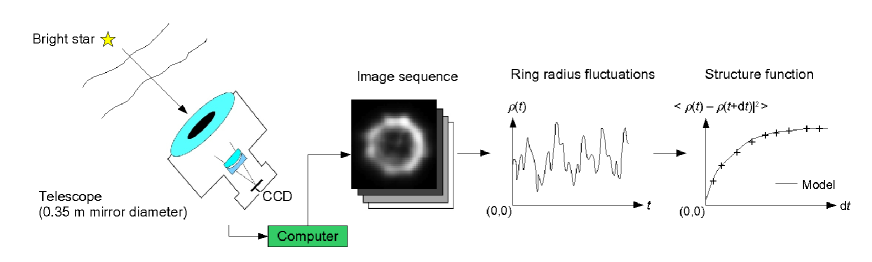
Figure 1: Overview of the FADE instrument and data analysis.

A new method for measuring the coherence time with a small telescope has recently been proposed in KT07. This method, termed FADE (FAst DEfocus), is based on recording and processing focus fluctuations produced by the atmospheric turbulence in a small telescope. The variance of defocus is proportional to $(D/r_{0})^{5/3}$ (Noll Noll (1976)) and gives a measure of the seeing, where $D$ is the telescope diameter. As shown in KT07, the variance of the speed of defocus is related to $\tau_{0}$ (this relation is given below in Sect. 3.4 where the derivation of $\tau_{0}$ from a sequence of fast defocus measurement is explained). In principle, $\tau_{0}$ can be obtained from the temporal analysis of almost any quantity affected by turbulence. However, tilts, the easiest to measure, are typically corrupted by telescope shake and guiding errors, hence are not suitable. The DIMM instrument is immune to the wind shake, but it is intrinsically asymmetric. An early attempt to extract $\tau_{0}$ from the DIMM signal by Lopez (Lopez92 (1992)) revealed the complexity of this approach and did not result in a practical instrument. If we discard tilts, the next second largest and slowest atmospheric terms are defocus and astigmatism. Defocus has angular symmetry and the rate of its variation is related to $\tau_{0}$. Attractive features of the FADE method thus are:

• direct measurement of $\tau_{0}$ and $\varepsilon_{0}$,

• use of the whole telescope aperture,

• immunity to tilts,

• small telescope size.

FADE can be useful for site testing and monitoring, but its feasibility has so far been demonstrated only by numerical simulation. Here we present an instrument implementing the new method.

The instrumental set-up is described in Sect. 2. Section 3 outlines the data analysis algorithm, while various instrumental effects are evaluated in Sect. 4 by numerical simulation. In Sect. 5 the seeing and coherence time measured with FADE are checked for consistency and are compared to simultaneous data from the DIMM and MASS instruments. Section 6 contains conclusions and an outline of further work. Mathematical derivations are given in Appendices A and B.

2 The instrument

2.1 Operational principle

The temporal structure function (SF) of atmospherically-induced focus variations $D_{4}(t)$ is related to the average wind speed in the atmosphere $\overline{V}$. The initial, quadratic part of SF is

$$D_{4}(t)\approx Ct^{2}\int_{0}^{+\infty}{\rm d}h\;C_{n}^{2}(h)\;V^{2}(h)=Ct^{2}\overline{V}_{2}^{2}\int_{0}^{+\infty}{\rm d}h\;C_{n}^{2}(h),$$ (1)

where the proportionality coefficient $C$ depends on the wavelength, telescope diameter and central obstruction (see KT07 and Appendix B for the derivation), $C_{n}^{2}(h)$ and $V(h)$ are vertical profiles of the refractive-index structure constant and wind speed. By measuring SF, we can estimate the integral in (1) that is similar to the integral entering the definition of $\tau_{0}$ (Roddier Roddier81 (1981)),

$$\tau_{0}=0.314r_{0}/\overline{V}_{5/3}=\left(118\lambda^{-2}\int_{0}^{+\infty}{\rm d}h\;C_{n}^{2}(h)\;V^{5/3}(h)\right)^{-3/5}.$$ (2)

The exponent of the wind speed is slightly different; however, we show below that fitting the measured SF to a theoretical model leads to a good estimation of $\tau_{0}$.

The defocus aberration can be measured with a wave-front sensor of any type or can be simply inferred from the size of a slightly defocused long-exposure stellar image (Tokovinin & Heathcote Donut (2006)). For FADE, a simple, fast, and accurate method is required. We chose to introduce a conic aberration into the beam in order to form a ring-like image. A small defocus slightly changes the radius of the ring. Ring-like images, “donuts”, are obtained by defocusing a telescope with a central obstruction. However, unlike a donut, the ring is fairly sharp in the radial direction, which means that the determination of the ring radius is largely insensitive to intensity fluctuations (scintillation) at the telescope pupil.

There is an inherent similarity between FADE and DIMM. In a DIMM, two peripheral beams are selected and are deviated by prisms to form an image of two spots. In FADE, the prisms are replaced by a conic aberration and the whole annular aperture is used to form a ring-like image instead of two spots.

The ring images are recorded by a fast CCD detector and stored on a computer disk (Fig. 1). They are processed offline to determine a temporal sequence of ring radii, $\rho(t)$, related to the defocus. In order to estimate the atmospheric parameters $\varepsilon_{0}$ and $\tau_{0}$, the temporal structure function of the defocus variations is computed (Eq. 14) and fitted to a model.

Atmospheric defocus fluctuations are fast: their temporal correlations decrease with a half-width 0.3 times the aperture crossing time $t_{\rm cross}=D/V$, i.e. with 2.2 ms for a telescope diameter $D=0.36$ m and wind speed $V=50$ m/s (cf. Appendix B). To capture the focus variations of interest, an acquisition frequency $\nu\geq 500$ Hz (exposure time $<2$ ms) is required, which is attainable with today’s fast CCD detectors.

2.2 Hardware

Table 1: Components of the FADE instrument

Component	Description
Telescope	Celestron C14, $D=0.356$ m, $F=3.910$ m
Central obstruction	Circular mask of 150 mm diameter
Aberrator	PCX lenses (Linos 312321 & 314321),
	$d_{L}=25$ mm, $f_{L}=\pm 50$ mm
Detector	Prosilica GE 680, $640\times 480$,
	pixel 7.4 $\mu$m ($0.39^{\prime\prime}$)
Interface	Gigabit Ethernet IEEE 802.3 1000baseT
Computer & OS	Dell D410, Windows XP

We assembled the FADE prototype from readily available commercial components (Table1). A 36-cm telescope was selected. In a smaller telescope, the focus variations are smaller, $\langle a_{4}^{2}\rangle\propto D^{5/3}$, and faster, $t_{\rm cross}\propto D$, hence more difficult to measure. Use of a fast CCD – GE 680 from Prosilica – is critical for the instrument, because it permits continuous acquisition with an image frequency 740 Hz when a 100x100 subsection of the full frame (region-of-interest, ROI) is read out. The signal is digitized in 12 bits. With the lowest internal gain setting, 0 dB, the conversion factor 2.86 ADU per electron and the readout noise 38 ADU = 13.4 e were measured. According to the specifications, the maximum quantum efficiency (QE) is 0.5 electrons per photon at wavelength $\lambda=0.50\;\mu$m with a full-width half-maximum spectral response of roughly $\Delta\lambda=0.25\;\mu$m. Indeed, the measured fluxes from stars correspond to the overall system QE of 0.35–0.40, including atmospheric and optical losses.

2.3 Optics

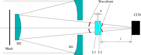
Figure 2: Optical layout of FADE (not to scale). The stellar light comes from left to right. After reflection from the telescope primary and secondary mirrors M1 and M2, the converging beam passes through the “aberrator” consisting of the lenses L1 and L2 and is detected by the CCD. The wave-front cross-sections before and after the aberrator are illustrated by thick line segments.

To create annular images, a conic aberration must be introduced into the beam. Conic lenses, axicons, have wide technical and research applications and are commercially available. In the case of FADE, we can successfully approximate a conic wave-front by a combination of a quadratic (defocus) and higher-order (spherical aberration) terms.

An aperture with a relative central obstruction $\epsilon$ gives a ring-like defocused image with the average angular radius $\rho=a_{4}\sqrt{48}/[D(1-\epsilon)]$, where $a_{4}$ is the defocus coefficient in linear units (throughout this article, the Zernike aberration coefficients are given in the Noll Noll (1976) notation). Such a ring can be sharpened by adding spherical aberration. Elementary analysis shows that for a relative central obstruction $\epsilon\sim 0.4$, the deviation from a conic surface is minimized when $a_{11}=-0.1\;a_{4}$. The rms error of this approximation is $0.01a_{4}$. In order to get a ring radius of $5^{\prime\prime}$ with a 35-cm telescope, we need the defocus amplitude $a_{4}\approx 600$ nm; hence, the difference of the approximated wave-front from a perfect cone will be 6 nm, or $\lambda/80$ at $\lambda=500$ nm.

To attain the desired aberration, we used an assembly of two simple plano-spherical lenses with equal but opposite curvature radii, which can be seen as a plane-parallel plate containing a meniscus-shaped void (Fig. 2). The thickness of the meniscus is adjusted by changing the gap $g$ between the lenses. The positive lens is closer to the primary mirror, so that the meniscus curvature opposes the curvature of the wavefront. We used lenses with focal lengths $f_{L}=\pm 50$ mm and a gap $g=0.7$ mm. When this element is placed at distance $l=93.5$ mm in front of the detector and the telescope is suitably refocused, a ring image of radius $\rho\approx 5^{\prime\prime}$ is formed. Optical modeling in Zemax shows that this “aberrator” is reasonably achromatic. The spherical aberration is proportional to $g\,l^{6}$, therefore it can be adjusted over a wide range. To block the inner part of the wavefront where it deviates from the cone, a central obstruction of 150 mm diameter, i.e. a relative diameter $\epsilon=0.42$, was placed at the telescope entrance. Obviously, there are many other possible optical arrangements to obtain wave-fronts with spherical aberration.

The average ring image in the real FADE instrument (Fig. 3) shows marked aberrations other than conical, caused by the defects of optical surfaces and of alignment. Similar rings were reproduced in our simulations with a combination of coma and higher-order aberrations (cf. Sect. 4.2). We also fitted the Zernike aberrations directly using the donut method (Tokovinin & Heathcote Donut (2006)) and found that the coma coefficient could reach $\sim$100 nm (1.2 rad). Furthermore, the defocus was not always kept at its optimum value as required for sharp ring images. The effect of such aberrations is studied in Sect. 4.4 by simulation.

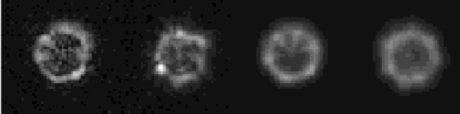
Figure 3: From left to right: Simulated ring image – Image of Sirius – Average of 1024 simulated images – Average of 1024 Sirius images. The sequence of Sirius images was recorded on Nov. 2 at 6:46 UT. The parameters for the data and simulations are given in Sect. 4.2.

2.4 Acquisition software

Since the GE 680 detector is relatively new, with no readily available software development kits as yet, we used the commercial software, Streampix from Prosilica. It provides all necessary functions for detector control and data storage in the FITS format, but the parameters need to be set manually at each acquisition, which requires constant attention. And they are not logged into the FITS headers or otherwise. Thus, Streampix is only a temporary solution. We checked that the image sequence is acquired at regular intervals, without time jitter. The detector was exposed for this purpose to a strictly periodic light signal at 10 Hz, and a $100\times 100$ ROI was read at 400 Hz. The power spectrum of the flux calculated from these data is a narrow peak at $(10.0\pm 0.2)$ Hz without significant tails.

2.5 Observations

The FADE instrument was installed in the USNO dome of the Cerro Tololo Inter-American Observatory (CTIO) in Chile for the period October 27 to November 3, 2006. The instrument was elevated $\sim 4$ m above the ground. We pointed FADE at bright stars, Fomalhaut ($\alpha$ PsA, A3V, $m_{V}=1.16$) in the evening, then Sirius ($\alpha$ CMa, A1V, $m_{V}=-1.47$). The exposure time ranged from 1 ms to 1.9 ms for Fomalhaut and was $<0.5$ ms for Sirius to avoid saturation. Figure 3 shows typical instantaneous and average images of Sirius, as well as simulated images. During our test run, the seeing was not very good at roughly $1^{\prime\prime}$, and the turbulence in the high atmosphere was strong and fast, as shown by the MASS data.

3 Data analysis

A correct algorithm of data processing and interpretation is critical for deriving the atmospheric parameters $\varepsilon_{0}$ and $\tau_{0}$. We carefully selected the most robust method of calculating atmospheric defocus from the ring-like images and used numerical simulation to study the influence on the results of various instrumental effects and of optical propagation (Sect. 4 below).

3.1 Estimating the ring radius

The center of gravity of the image $(x_{c},y_{c})$ is calculated by the usual formula

$$x_{c}=\sum_{l,k}x_{l,k}\;I_{l,k}/\sum_{l,k}I_{l,k}\hskip 14.45377pt{\rm and\/}\hskip 14.45377pty_{c}=\sum_{l,k}y_{l,k}\;I_{l,k}/\sum_{l,k}I_{l,k}.$$ (3)

The ring radius $\rho$ can then be estimated in a similar way, as the intensity-averaged distance from this center:

$$\rho=\sum_{l,k}r_{l,k}\;I_{l,k}/\sum_{l,k}I_{l,k}.$$ (4)

Here $I_{l,k}$ is the light intensity at pixel $(l,k)$, and $r_{l,k}$ is the distance of this pixel from the center. There are various caveats below the apparent simplicity of this procedure.

There is no unambiguous way to assign a center to a real (distorted and noisy) ring image. A simple center-of-gravity is a very rough estimate of $(x_{c},y_{c})$; in particular, it is affected by the intensity fluctuations in the ring due to scintillation. It is better to compute $(x_{c},y_{c})$ with clipped intensities: 0 below a threshold and 1 above, the threshold being set safely above the background and its fluctuations. This initial estimate can be improved further by minimizing the intensity-weighted mean distance of the pixels from the ring, as described in Appendix A. However, small inaccuracies in the center determination do not affect the resulting radius critically, and in fact, we found the initial estimate to be adequate.

A second caveat concerns the choice of the pixels used for the radius estimate. A considerable fraction of pixels lie outside the ring in an empty area that only contributes noise. To reduce the noise with a minimal loss of information, we restricted the pixels used in (4) to a mask of inner radius $\overline{\rho}-\Delta\rho$ and outer radius $\overline{\rho}+\Delta\rho$, where $\overline{\rho}$ is the average ring radius. We express the mask half-width $\Delta\rho$ as a fraction $\delta$ of the diffraction half-width of the ring,

$$\Delta\rho=\delta\;\lambda/[0.5\;D\;(1-\epsilon)].$$ (5)

Figure 4 shows that a mask with $\delta=2$ would be good for an ideal, diffraction-limited ring. For a typical image sequence, however, the ring is widened by telescope aberrations and atmospheric distortions, so we set $\delta=4$, which covers the actual ring image with a sufficiently conservative, but still reasonable, margin.

Figure 4: Total intensity inside concentric circles of radii $\rho$ for the average of 1024 centered images. Full line: sequence of Fomalhaut images recorded on Nov. 2. Dashed line: simulated diffraction-limited ring images (see Table 2).

The simulations show that scintillation and aberrations add to the fluctuations of the estimated radii and thus bias the results of FADE. To reduce this effect, we subdivide the ring into eight 45^∘ sectors and – utilizing the same center estimate $(x_{c},y_{c})$ – apply Eq. 4 to each sector separately, and then average the result. This reduces the effect of azimuthal intensity variations. An added advantage of the procedure is that the relative variance $s$ of the total intensities in the sectors $I_{k}$ with respect to their average $\overline{I}_{k}$ serves as a measure of the scintillation, hence of the turbulence height,

$$s = \frac{1}{8}\sum_{k=1}^{8}(I_{k}-\overline{I}_{k})^{2}\;/\;\overline{I}_{k}\;^{2}.$$ (6)

The method of calculating the ring parameters $(x_{c},y_{c},\rho)$ is less rigorous than fitting a wave-front model directly to the image. The big advantage of the estimator (4), however, is its simplicity.

3.2 Noise and limiting stellar magnitude

The errors of the radius estimates caused by photon and readout noise are obtained by differentiating Eq. (4) and using the independence of the noise in each pixel:

$$\sigma^{2}_{\rho,{\rm noise}} = \left(\frac{\sigma_{\rm ron}}{N_{\rm ph}}\right)^{2}\sum_{l,k}(r_{l,k}-\overline{\rho})^{2}+\frac{\delta^{2}_{\rho}}{N_{\rm ph}},$$ (7)

$$\delta^{2}_{\rho} = \sum_{l,k}I_{l,k}\;(r_{l,k}-\overline{\rho})^{2}\;/\;N_{\rm ph}.$$ (8)

Here, $\sigma_{\rm ron}$ is the rms detector noise, $N_{\rm ph}=\sum_{l,k}I_{l,k}$ the total stellar flux in one exposure (both in electrons), $\overline{\rho}$ the average ring radius, and $r_{l,k}$ is the distance of pixel $(l,k)$ from the center, expressed either in pixels or arc-seconds. The rms ring-width $\delta_{\rho}$ quantifies the ring sharpness, which turns out to be critical for getting unbiased measurements with FADE (see Sect. 4.4). The summation is extended only over pixels inside the mask, as described in Sect. 3.1. We recognize a familiar sum of the readout noise (first term) and photon noise (second term), where the first term typically dominates. Equation (7) does not account for such additional noise sources as scintillation, image distortion, etc.

Formula (7) is useful for predicting the limiting magnitude of FADE. A star of zero $V$-magnitude gives a flux $N_{\rm ph}\sim 6\cdot 10^{5}$ photo-electrons in 1 ms exposure in our instrument. The rms noise on the radius estimate with plausible parameters ($\rho=5^{\prime\prime}$, $\sigma_{\rm RON}=13$, $\delta=4$) is then about 2 mas. It will increase to 20 mas for a star with $m_{V}=2.5^{m}$ – still much less than the atmospheric signal. Despite very short exposures, FADE is not photon-starved.

3.3 The response coefficient of FADE

The relation between the ring radius fluctuations $\Delta\rho$ and the atmospheric defocus (Zernike coefficient $a_{4}$) is intuitively clear. But what is the exact coefficient $A$ in the formula $\Delta\rho=Aa_{4}$? Recall that the atmsopheric defocus $a_{4}$ is related to the phase distortion $\varphi({\bf r})$ as

$$a_{4}=\int{\rm d}^{2}{\bf r}\;z_{4}({\bf r})\;\varphi({\bf r}),$$ (9)

where ${\bf r}$ is the normalized coordinate vector on the pupil and $z_{4}({\bf r})$ the orto-normal Zernike defocus given by Noll (Noll (1976)) for the circular aperture and in Fig. 5 for the annular aperture.

Defocus $z(r)=\sqrt{12}\left(r^{2}-\frac{1+\epsilon^{2}}{2}\right)/(1-\epsilon^{2})$ Cone $z(r)=\left[r-\frac{2(1-\epsilon^{3})}{3(1-\epsilon^{2})}\right]\left[\frac{1+\epsilon^{2}}{2}-\frac{4(1-\epsilon^{3})^{2}}{9(1-\epsilon^{2})^{2}}\right]^{-1/2}$ Gradient $z(r)=\left[\frac{\delta(r-1)}{2\pi r}-\frac{\delta(r-\epsilon)}{2\pi\epsilon r}\right]$

Figure 5: Response functions $z(r)$ on annular aperture for Zernike defocus, conic aberration, and average radial gradient. The first two functions are normalized in the Noll (Noll (1976)) sense. The coefficients $a_{4}$, $a_{c}$, and $a_{g}$ are calculated as integrals (9). Here $\delta$ is the Dirac’s delta function.

A reaction of our simple radius estimator (4) to a small perturbation of phase and amplitude at the telescope pupil can be determined analytically (cf. Perrin et al. Perrin (2003) for an example of similar analytics). It turns out that the response to a phase perturbation in the pupil plane is not exactly proportional to the Zernike defocus. Moreover, it depends on the adopted mask half-width $\delta$. For $\delta\sim 1$, the response resembles a cone, so that FADE measures something similar to a conic aberration. On the other hand, for $\delta\geq 2$ the computed ring radius is related to the average radial gradient of the wave-front, and therefore FADE measures the difference $a_{g}$ between the phase averaged on the outer and inner edges of its annular aperture. Its response is further modified when the ring is distorted by aberrations. In this case, the radius estimate is sensitive to both amplitude and phase fluctuations. Although we developed a full analytical treatment of this problem, it is omitted here for the sake of simplicity.

The three quantities – Zernike defocus $a_{4}$, conic aberration $a_{c}$, and average phase gradient $a_{g}$ – are similar, especially on the annular aperture (Fig. 5). FADE measures something else, but its response is most closely approximated by $a_{g}$ when the ring radius is calculated with a large mask width $\delta$. Let $a_{g}$ be the average phase difference between the outer and inner borders of the aperture, the corresponding change of the angular ring radius is then

$$\Delta\rho=\frac{a_{g}\;\lambda}{\pi D(1-\epsilon)}.$$ (10)

The Zernike defocus on the annular aperture is proportional to $a_{4}\sqrt{12}r^{2}/(1-\epsilon^{2})$, where $r$ is normalized by the pupil radius. Hence, $a_{g}=a_{4}\times\sqrt{12}$, and the proportionality coefficient $A$ follows from Eq. (10),

$$\Delta\rho=A\;a_{4}=a_{4}\frac{\lambda}{\pi D}\;\frac{\sqrt{12}}{1-\epsilon}.$$ (11)

The atmospheric variance of the defocus $a_{4}$ or gradient $a_{g}$ on an annular aperture can be computed, as done by Noll (Noll (1976)) for a filled aperture. Alternatively, the variance of the ring radius may be directly written as

$$\sigma_{\rho}^{2}=C_{\rho}(\lambda/D)^{2}(D/r_{0})^{5/3}$$ (12)

analogous to similar formulae for the gradient or Zernike tilt. Our numerical calculation for the average-gradient response (see Eq. 10) leads to an approximation valid for $\epsilon<0.6$ with an accuracy of $\pm 7\,10^{-5}$:

$$C_{\rho}\approx 0.03288+0.0503\epsilon-0.05638\epsilon^{2}+0.04056\epsilon^{3}.$$ (13)

We studied the response of FADE by analytical calculation and numerical simulations and found that the exact coefficient $C_{\rho}$ in Eq. 12 depends on all parameters of the instrument and data processing. A choice of $\delta\geq 2.5$ ensures a relative stability of the response with respect to small aberration, propagation, etc. A small correction to the “ideal” response coefficient is finally determined by simulation (Sect. 4.3) and applied to the real data.

The lack of a unique, well-established coefficient relating measurements to atmospheric parameters may appear disturbing. However, a similar analysis applied to the classical DIMM instrument leads to the conclusion that its response, too, depends on the details of centroid calculation and, furthermore, is modified by propagation and optical aberrations. In this respect, FADE and DIMM are not different.

Table 2: Simulation parameters.

	$N$	$\nu$	d$t$	$m_{V}$	$\sigma_{\rm ron\/}$	$\rho$	$a_{4}$	$a_{7}$	$a_{11}$	$a_{27}$	$h$	$\varepsilon_{0}$	$\overline{V}$
		Hz	ms		el.	′′	rad	rad	rad	rad	km	′′	m/s
Fig. 3	1024	700	0.15	-1.5	17	3.8	0	0.7	-0.75	0.3	13	1.05	17
Fig. 4	1024	700	0.15	-1.5	17	5.5	0	0	0	0	5	1.00	17
Eq. 20	1024	700	0.15	-1.5	17	3.8	0	0	0	0	10	var.	35
Fig. 7 top	1024	700	0.15	-1.5	17	0	12	0.7	var.	0.3	0	var.	35
Fig. 7 bottom	1024	700	0.15	-1.5	17	0	12	0.7	var.	0.3	5	var.	35
Fig. 8 left	1024	700	1.4	var.	17	4	0	0	0	0	5	var.	35
Fig. 8 middle	1024	700	0.15	-1.5	17	var.	0	0	0	0	5	var.	35
Fig. 8 right	1024	700	0.15	-1.5	17	4	0	var.	0	0	5	var.	35

3.4 Derivation of the seeing and coherence time

Figure 6: Structure function of focus variations measured at 700 Hz (crosses) fitted with a model of three turbulent layers (line).

We convert the measured ring radius into defocus using coefficient $A$ (see Eq. 11) and calculate the temporal structure function of defocus $D_{4}(t)$,

$$D_{4}(t)=\langle[a_{4}(t^{\prime}+t)-a_{4}(t^{\prime})]^{2}\rangle.$$ (14)

A typical SF is plotted in Fig. 6. A theoretical expression for the defocus SF has been derived in KT07. We generalize it to annular apertures in Appendix B. The initial, quadratic part of SF is directly related to the combined time constant $\tau_{0}$ of all turbulent layers. However, the acquisition frequency is not fast enough to capture the initial quadratic part of SF extending only to time lags of $<0.1t_{\rm cross}$. In order to get two points on this part for a layer moving with $V=50$ m/s, a frame rate of $\sim 3$ kHz would be required.

To overcome the sampling problem, we fit the initial part of SF to a model of $N$ turbulent layers with Fried parameters $r_{0,i}$ and velocities $V_{i}$, $1\leq i\leq N$:

$$D_{4}(t>0)=1.94D^{5/3}\sum_{i=1}^{N}r_{0,i}^{-5/3}K_{4}(2tV_{i}/D,\epsilon)+\frac{2\,\sigma^{2}_{\rho,{\rm noise}}}{A^{2}},$$ (15)

where the function $K_{4}(\beta,\epsilon)$ is defined in Appendix B and $\sigma^{2}_{\rho,{\rm noise}}$ is the noise of the radius estimate determined by Eq. 7. The adjusted parameters are $r_{0,i}$ and $V_{i}$. As will be seen in Sect. 5.1, the estimate of $\tau_{0}$ is independent of $N$ if $N\geq 3$. Accordingly, a three-layer model is chosen for the data analysis (Fig. 6). We fit only the initial part of SF, up to the time increment $\Delta t$. Its exact value is not critical, as long as it is large enough for unambiguous fitting of the parameters, $\Delta t\,\nu>2N+1$. For further data analysis, we set $\Delta t=40$ ms.

The atmospheric parameters $(r_{0},\overline{V},\tau_{0})$ are calculated as

$$r_{0}^{-5/3} = \sum_{i=1}^{N}r_{0,i}^{-5/3},$$ (16)

$$(\overline{V}/r_{0})^{5/3} = \sum_{i=1}^{N}(V_{i}/r_{0,i})^{5/3},$$ (17)

$$\tau_{0} = 0.314\;r_{0}/\overline{V}.$$ (18)

The estimate of $r_{0}$ is also obtained directly from the ring-radius variance $\sigma^{2}_{\rho}$ by subtracting the noise,

$$\sigma_{\rho}^{2}-\sigma^{2}_{\rho,{\rm noise}}=C_{\rho}(\lambda/D)^{2}(D/r_{0})^{5/3}.$$ (19)

When SF reaches its asymptotic value on time increments smaller than 40 ms, the same value of $r_{0}$ is derived from the ring-radius variance (Eq. 19) and from the model (Eq. 16). The robustness of parameter estimates derived by model fitting has been confirmed by numerical simulation (Sect. 4) and by fitting alternative models to real data (Sect. 5.1).

4 Simulations

A new seeing monitor can be validated by comparing it with another, well-established instrument. In the case of FADE, however, there is no reliable comparison data on $\tau_{0}$. Instead, we simulated our instrument numerically as faithfully as we could and studied the influence of various instrumental and data-reduction parameters on the final result.

Figure 7: Influence of the ring sharpness – quantified in terms of the ring width $\delta_{\rho}$ – on the seeing and coherence time estimates. Top – turbulence layer at ground level, bottom – turbulence layer at 5 km altitude. Simulation parameters are given in Table 2.

Figure 8: Dependence of the seeing and coherence time estimates on stellar magnitude $m_{V}$, mean ring radius $\rho$, and coma aberration $a_{7}$. Simulation parameters are given in Table 2.

4.1 Simulation tool

Our simulation tool generates the complex amplitude of the light field propagated through one or several phase screens with Kolmogorov spectrum. The screens are typically 1024² pixels with 1 cm sampling, i.e. about 10 m across. The resulting amplitude pattern is periodic, without edge effects. It is “dragged” in front of the simulated telescope with a chosen wind speed, wrapping around edges in both coordinates and eventually covering the whole area. The monochromatic images created by a telescope with a perfect conic aberration of specified amplitude and, possibly, some additional intrinsic aberrations are re-binned into the detector pixels, distorted by readout and photon noise and fed to the data-analysis routine instead of the real data. Our tool has been verified by comparing with analytical results for weak perturbations and has been used for simulating other instruments such as DIMM and MASS. The limitations of this tool are the monochromatic light, single wind velocity for all layers, and instantaneous exposure time.

We used two alternative, nearly equivalent ways of producing ring images. In the first method, a perfect conic wavefront was generated, and its amplitude was expressed as a ring radius $\rho$. In the second method, we do not apply conic aberration ($\rho=0$), but instead select a combination of defocus and spherical aberrations to mimic a real telescope. The sense of the Zernike coefficients $a_{4}$ and $a_{11}$ in both cases is distinct.

4.2 Parameters of the simulations

For convenience, the simulation parameters are gathered in Table 2. These parameters are:

• number of images in the sequence $N$,

• acquisition frequency $\nu$,

• exposure time d$t$,

• visual stellar magnitude $m$,

• readout noise $\sigma_{\rm ron\/}$,

• conic aberration quantified by the average ring radius $\rho$,

• amplitudes of the Zernike aberrations $a_{4}$ (defocus), $a_{7}$ (coma), $a_{11}$ (spherical), and $a_{27}$,

• altitude of the single turbulent layer $h$,

• seeing $\varepsilon_{0}$,

• wind speed $\overline{V}$.

Simulated ring images are compared in Fig. 3 to the images of Sirius recorded on Nov. 2. The combination of exposure time and magnitude results in the detected flux of $3\cdot 10^{5}$ electrons per simulated image, as in the actual images of Sirius. For this sequence, the estimated turbulence parameters equal: $\varepsilon_{0}=1.05",\;\overline{V}=17$ m/s, $\tau_{0}=1.86$ ms (Fig. 6). The same parameters are chosen for the simulated images. For the closest resemblence between simulated and real images, telescope aberrations are set to $a_{7}=0.7$ rad, $a_{11}=-0.75$ rad, $a_{27}=0.3$ rad. The turbulence is placed at 13 km altitude to reproduce the actual level of scintillation, evaluated from the intensity variance between ring sectors $s=0.011$ (cf. Eq. 6).

4.3 Refining the response coefficient

The coefficient $A$ relating radius variation to defocus is given by Eq. 11. Its actual numerical value, however, depends on the method of radius estimation and, in particular, on the choice of the mask width $\delta$. For $\delta=4$, we determined it to equal 1.077 by comparing $\tau_{0}$ estimates from sequences of simulated images, to the nominal input value of $\tau_{0}$ when Eq. 11 is used to relate the radius to defocus. The corresponding simulation parameters are summarized in Table 2. Thus,

$$\Delta\rho/a_{4} = 1.077\;\frac{\lambda}{\pi D}\;\frac{\sqrt{12}}{1-\epsilon}.$$ (20)

4.4 Instrumental biases

The data analysis relies on radius estimates that can be altered by telescope aberrations, scintillation, detector and photon noise, etc. Here we evaluate the instrumental bias by changing some parameters, while other parameters are fixed. In each case, a sequence of 1024 simulated images is generated with the parameter values listed in Table 2. The wind speed is set to 35 m/s and the coherence time is then changed by modifying the seeing.

Ring sharpness.

The ring is sharp in the radial direction when the wavefront is exactly conic. A good approximation of the conic wavefront is achieved by the optimum combination of defocus and spherical aberrations, $a_{11}=-0.1\,a_{4}$. Here we explore the effect of unsharp ring images by setting $a_{4}=12$ rad and varying $a_{11}$ about its optimum value $a_{11}=-1.2$ rad. Unlike the rest of the simulations, we do not apply conic aberration and set $\rho=0$. Wrong values of $a_{11}$ make the ring wider, as shown by its rms width, $\delta_{\rho}$ (Eq. 8).

As seen in Fig. 7, the seeing and coherence-time estimates are biased in the case of blurred rings and high-altitude turbulence. The sign of the bias depends on the sign of the deviation from the optimum $a_{11}$. When the turbulent layers are low, the scintillation is weak and the parameters are correctly derived even if the ring images are blurred.

To ensure a correct derivation under any atmospheric conditions, the ring width should be close to its diffraction-limited value $\delta_{\rho,0}$:

$$\delta_{\rho}<1.2\,\delta_{\rho,0}\;;\hskip 14.45377pt\delta_{\rho,0}=1.7\,\lambda/[D\,(1-\epsilon)],$$ (21)

where the coefficient 1.7 is determined from the width, $\delta_{\rho}=0.87^{\prime\prime}$, of diffraction-limited rings. Given the instrumental set-up, images should be rejected if $\delta_{\rho}<1^{\prime\prime}$. However, all images recorded with the FADE prototype have $\delta_{\rho}>1^{\prime\prime}$. Hence, we apply a softer data-selection criterion: $\delta_{\rho}<1.25^{\prime\prime}$, and note that the resulting estimates might still be biased if the turbulence was high.

Stellar magnitude, ring radius, and coma.

Figure 8 examines the stability of the seeing and coherence time estimates with respect to the stellar magnitude $m_{V}$, ring image radius $\rho$, and coma aberration $a_{7}$. In agreement with Eq. 7, estimates are correct up to stellar magnitudes 2–3. Spatial sampling and coma aberration do not affect the estimates if $\rho\geq 2^{\prime\prime}$ (i.e. 5 pixels) and $a_{7}\leq 2$ rad.

5 Analysis of observations

Seeing and coherence time were estimated from all sequences of 4000 images recorded with FADE at Cerro Tololo between October 29 and November 2, 2006. In this section, we check the FADE results for consistency and compare them with the MASS-DIMM.

5.1 Influence of instrumental parameters

During data acquisition, instrumental parameters were varied over a broad range to evaluate their effect on the results. Even though the non-stationarity of the atmosphere precludes direct comparisons, some conclusions can nevertheless be drawn.

The ring sharpness, $\delta_{\rho}$, has been identified as a major source of instrumental bias in FADE when significant high-altitude turbulence is present. In our data, most images have $1^{\prime\prime}<\delta_{\rho}<1.5^{\prime\prime}$, whereas a perfect diffraction-limited ring has $\delta_{\rho}=0.9^{\prime\prime}$. Analysis of the average ring images confirms that the optimum combination of defocus and spherical aberrations was not reached, $a_{4}$ and $a_{11}$ often having the same sign rather than opposite signs. For our data, the dispersion and mean of $\tau_{0}$ increase when $\delta>1.25^{\prime\prime}$; accordingly, sequences with $\delta_{\rho}>1.25^{\prime\prime}$ are disregarded. Still, some bias caused by radially defocused images remains.

Figure 9: Coherence time derived from the recorded data by fitting a model with $N=3$ layers (x-axis) compared to the coherence time derived with $N=2$ (dotted line) and $N=4$ (solid line) models.

As described in Sect. 3.4, the data are fitted to a model with a discrete number of turbulent layers, $N$. What is the minimum value of $N$ that permits a correct derivation of $\tau_{0}$? Figure 9 shows that the $\tau_{0}$ values obtained with 3 and 2 (resp. 4) layers differ on average by 7% (resp. 2%). An average difference of 2% is likewise obtained when comparing the estimates with 3 and 5 layers. A 3-layer model is thus a good compromise enabling a fit to the data with only six parameters.

Figure 10: Coherence time derived from all sequences recorded with $\nu\geq 700$ Hz when every image (x axis) and every other image (y axis) is considered.

The influence of the acquisition frequency on the measured coherence time is examined in Fig. 10. The data sequences recorded at frequencies $\nu\geq 700$ Hz were re-analyzed considering every other image. The coherence time obtained with a slower $\nu/2$ sampling is on average 9% longer than with the fast sampling. This difference is reproduced by simulations if the turbulence is placed at 5 km altitude and if the ring-images are slightly defocused in the radial direction ($a_{11}/a_{4}\approx-0.07$ or $-0.14$ instead of $a_{11}/a_{4}=-0.11$ corresponding to a sharp ring). The effect of temporal under-sampling is perceptible if the same comparison is repeated with sequences recorded at frequencies below 700 Hz: the number of points on the initial, increasing part of SF is then not always sufficient to unambiguously extract the six fitted parameters, and the coherence time is poorly constrained. To ensure a correct temporal sampling under fast turbulence, we ignored the sequences with $\nu<500$ Hz.

In line with the simulations, the coherence time estimates do not depend on the average ring image radius. Similarly, the parameter statistics seem unbiased by the stellar flux and by the exposure time. While the sequences of Sirius ($m_{V}=-1.5$) and Fomalhaut ($m_{V}=1.2$) images were recorded with exposure times of d$t<0.5$ ms and $1.0<{\rm d}t<1.9$ ms, respectively, no obvious difference exists between the mean and rms of the atmospheric parameters measured in terms of these two stars,
$\epsilon_{0}^{\rm S}:\;(0.9\pm 0.2)^{\prime\prime}\hskip 28.90755pt\epsilon_{0}^{\rm F}:\;(0.8\pm 0.1)^{\prime\prime}$
$\tau_{0}^{\rm S}:\;(1.4\pm 0.5)$ ms       $\tau_{0}^{\rm F}:\;(1.3\pm 0.5)$ ms.

5.2 Comparison with MASS and DIMM

In this section, the seeing and coherence time obtained with FADE are compared to simultaneous measurements by the CTIO site monitor located at 10 m distance from FADE on a 6 m high tower. The monitor consists of a combined MASS-DIMM instrument fed by the 25-cm Meade telescope and looking at bright ($V=2^{m}...3^{m}$) stars near zenith. Of particular interest here is the time constant $\tau_{0}$ estimated by MASS from the temporal characteristics of scintillation by the method of Tokovinin (MASS_tau (2002)). This method is intrinsically biased because it does not account for the turbulence below $\sim 500$ m. Moreover, it has been recently established by simulations that the coefficient used to calculate $\tau_{0}$ in the MASS software must be increased by 1.27. In the following, we correct $\tau_{0}$ by applying this coefficient and including the contribution of the ground layer:

$$\tau_{0}^{-5/3} = (1.27\;\tau_{\rm MASS\/})^{-5/3}+118\,\lambda^{-2}\,V^{5/3}_{\rm GL\/}\,(C_{\rm n}^{2}\,{\rm d}h)_{\rm GL}.$$ (22)

The turbulence integral in the ground layer, $(C_{\rm n}^{2}\,{\rm d}h)_{\rm GL\/}$, is computed from the difference between the turbulence integrals measured by DIMM (whole atmosphere) and MASS (above 500 m), while the ground layer wind speed, $V_{\rm GL\/}$, is known from the local meteorological station. Even after correction by Eq. (22), the coherence time measured by MASS-DIMM should be taken with some reservation because it has never been checked against independent instruments and some bias is possible.

Figure 11 compares the estimates of $\varepsilon_{0}$ and $\tau_{0}$ obtained with FADE from October 29 to November 2 to the results of MASS-DIMM. We do not expect detailed correlation, because the instruments were sampling different atmospheric volumes. As seen in Fig. 11, the seeing measurements are better correlated than the coherence times.

Statistically, it appears that FADE slightly underestimates the seeing. This effect is reproduced with simulations of high-altitude turbulence if the ratio of spherical aberration to defocus $a_{11}/a_{4}$ is set higher than its optimum value $-0.1$ corresponding to sharp ring images. In this case, FADE also underestimates the coherence time. The bias on $\tau_{0}$ can, however, not be ascertained by Fig. 11 because the $\tau_{0}$ estimates by MASS might likewise be biased. Thus, the comparison presented in this section cannot be considered as a validation of FADE.

Figure 11: Seeing and coherence time measured with FADE between October 29 and November 2, compared to simultaneous measurements by the MASS-DIMM. The average values and standard deviations of parameters and the correlation coefficients are indicated.

6 Conclusions and perspectives

We have built a first prototype of the site-testing monitor, FADE, suitable for routine measurements of the atmospheric coherence time $\tau_{0}$, as well as the seeing $\varepsilon_{0}$. The instrument was tested on the sky. Extensive simulations substantiate the validity of the FADE results and indicate potential instrumental biases. Our main conclusions are as follows:

• The sampling time of the image sequence must be a small fraction of the aperture crossing time $t_{\rm cross}=D/V$ ($\sim$10  ms for $D=0.36$ m and wind speed $V=36$ m/s). Sampling at $\nu\geq 500$ Hz appears adequate under most conditions.

• The sharpness of the ring image in the radial direction does not bias the results when the turbulence is located near the ground. But it can bias both $\tau_{0}$ and $\varepsilon_{0}$ estimates when high layers dominate, and strict control of the telescope aberrations is thus required. The aberrations (hence the data validity) can be evaluated a posteriori from the average ring image. Real-time estimates of the ring radius $\rho$ and width $\delta_{\rho}$ are needed to ensure good optical adjustment of the instrument.

• The FADE monitor with 36-cm telescope can work on stars as faint as $m_{V}=3^{m}$.

• A simple estimator of the ring radius (Eq. 4) is adequate and robust, provided a wide enough mask around the ring ($\delta\sim 4$) is used in the calculation.

• Moderate telescope aberrations such as coma are acceptable. The results are not critically influenced by small telescope focus errors.

The current FADE prototype stores all image sequences, leading to a large data volume; the data are processed offline. While this procedure was necessary for the first experiments, online processing will be implemented in a definitive instrument. We have formulated and tested the data processing algorithm and can now develop adequate real-time software.

We plan to develop an improved version of FADE with real-time data analysis. It will be compared to simultaneous estimates of the atmospheric time constant from currently working adaptive-optics systems (Fusco et al. Fusco2004 (2004)) and/or long-baseline interferometers such as VLTI. Characterization of Antarctic sites for future interferometers is an obvious application for FADE.

Appendix A Estimator of the ring radius and center

The parameters of the ring-like image – its center $(x_{c},y_{c})$ and radius $\rho$ – can be derived by minimizing the intensity-weighted mean squared distance of the pixels from the circle, $\delta^{2}_{\rho}$:

$$\delta^{2}_{\rho} = \sum_{l,k}I_{l,k}\;(r_{l,k}-\rho)^{2}\;/\;\sum_{l,k}I_{l,k},$$ (23)

where $r_{l,k}=[(l-x_{c})^{2}+(k-y_{c})^{2}]^{0.5}$ is the distance of pixel $(l,k)$ from the ring center, $(x_{c},y_{c})$. Setting the partial derivative of $\delta^{2}_{\rho}$ over $\rho$ to zero, we obtain the radius estimator of Eq. 4. However, it still depends on the unknown parameters $(x_{c},y_{c})$. By use of Eq. 4, Eq. 23 is simplified to:

$$\delta^{2}_{\rho} = \frac{\sum_{l,k}I_{l,k}r_{l,k}^{2}}{\sum_{l,k}I_{l,k}}-\;\left[\frac{\sum_{l,k}I_{l,k}\;r_{l,k}}{\sum_{l,k}I_{l,k}}\right]^{2}.$$ (24)

This formula does not contain $\rho$. The center coordinates $(x_{c},y_{c})$ can be derived by setting the partial derivatives of $\delta^{2}_{\rho}$ over parameters to zero and solving the equations. We determine the center numerically by minimizing Eq. 24 and using the center-of-gravity coordinates as a starting point.

Appendix B Structure function of atmospheric defocus

The temporal structure function of atmospherically-induced defocus variations – Zernike coefficient $a_{4}$ in Noll’s (Noll (1976)) notation – has been derived in KT07 for a filled circular aperture. Here we generalize it to an annular aperture. Without repeating the whole derivation, we refer the reader to KT07 and modify only the spatial spectrum of the Zernike defocus, taking the central obstruction ratio $\epsilon$ into account. The resulting expression is

$$D_{4}(t) = 0.821\;k^{2}D^{5/3}\int_{0}^{+\infty}{\rm d\/}h\;C_{\rm n}(h)^{2}\;K_{4}\left(\frac{2tV(h)}{D},\epsilon\right),$$ (25)

$$K_{4}(\beta,\epsilon) = \frac{12}{\;(1-\epsilon^{2})^{4}}\;\int_{0}^{+\infty}{\rm d\/}x\;x^{-8/3}\;[1-J_{0}(\beta x)]\;$$ (26)

$$\times \left[\frac{J_{3}(x)}{x}-\epsilon^{4}\frac{J_{3}(\epsilon x)}{\epsilon x}+\;\epsilon^{2}\frac{J_{1}(x)}{x}-\epsilon^{2}\frac{J_{1}(\epsilon x)}{\epsilon x}\right]^{2},$$

where $k=2\pi/\lambda$, $J_{n}$ is the Bessel function of order $n$, $C_{\rm n}(h)^{2}$ and $V(h)$ are the altitude profiles of the refractive-index structure constant and wind speed, respectively. Considering the known relation between the turbulence integral and the Fried parameter, $r_{0}^{-5/3}=0.423\,k^{2}\,C_{\rm n}^{2}{\rm d}h$, we can also write the defocus SF produced by a single layer as

$$D_{4}(t)=1.94\,(D/r_{0})^{5/3}K_{4}(2tV/D,\epsilon).$$ (27)

For calculating the function $K_{4}$, it is convenient to approximate the integral (26) by an analytical formula, as in KT07. We suggest the approximation

$$K_{4}(\beta,\epsilon)\approx\frac{C_{1}\,\beta^{2}+C_{2}\,\beta^{6}}{1+C_{3}\,\beta^{\alpha}+\beta^{6}},$$ (28)

where the coefficients are cubic polynomials of $\epsilon$:

$$C_{i}=C_{i,0}\sum_{k=0}^{3}c_{i,k}\,\epsilon^{k},$$ (29)

cf. Table 3. This approximation is valid for $\epsilon<0.6$ with a maximum relative error of less than 5% (3% for $\epsilon=0.42$) and correct asymptotes. The asymptotic value $K_{4}(\infty,\epsilon)=C_{2}$ gives the focus variance on annular aperture, analogous to the Noll’s coefficient. For $\epsilon=0$, we get $C_{2}=0.024$ and the focus variance coefficient of $1.94\times 0.024/2=0.0233$, in agreement with Noll’s result.

Table 3: Coefficients of (28)

Param.	$C_{0}$	$\epsilon^{0}$	$\epsilon^{1}$	$\epsilon^{2}$	$\epsilon^{3}$
$C_{1}$	0.04642	1	$-$0.182	$-$2.431	2.028
$C_{2}$	0.0240	1	$-$0.017	$-$3.619	2.833
$C_{3}$	1	1.25	0	0	7.5
$\alpha$	1	2.18	$-0.93$	0	0

The function $K_{4}(\beta,\epsilon)$ reaches half its saturation value at $\beta=0.63$; hence, the atmospheric defocus correlation time is $\sim 0.3D/V$, as is well known in adaptive optics.

The above analysis is valid for instantaneous measurements, while the defocus is in fact averaged over the exposure time. This effect is usually non-negligible for the DIMM. The time averaging can be included as an additional factor in the integral (26), as done e.g. in Tokovinin (MASS_tau (2002)). We made this calculation and found that the initial, quadratic part of $D_{4}(t)$ (or, equivalently, the parameter $C_{1}$ in Eq. 28) is reduced by 0.8 for an exposure time $t_{\rm exp}\sim 0.3D/V$ and a layer moving with the speed $V$. To adequately sample the SF features produced by the fastest-moving layers, the sampling time (hence exposure time) must be shorter than $0.3D/V_{\rm max}$, so the bias caused by the finite exposure in FADE can be neglected. In hindsight, this result could be expected: to follow the focus variations, we need such a fast sampling that the integration during the sampling period has a negligible effect.

References

- (1) Fusco, T., Ageorges, N., Rousset, G., Raboud, D., Gendron, E., Mouillet, D., Lacombe, F. et al. 2004, Proc. SPIE, 5490, 118
- (2) Kellerer, A., & Tokovinin, A. 2007, A&A, 461, 775 (KT07)
- (3) Kornilov, V., Tokovinin, A., Vozyakova, O., Zaitsev, A., Shatsky, N., Potanin, S., & Sarazin, M. 2003, Proc. SPIE, 4839, 837
- (4) Lopez, B. 1992, A&A, 253, 635
- (5) Noll, R. 1976, J. Opt. Soc. Am., 66, 207
- (6) Perrin, M.D., Sivaramakrishnan, A., Makidon, R.B. et al. 2003, ApJ, 596, 702
- (7) Roddier, F. 1981, Progress in Optics, 19, 281
- (8) Sarazin, M., & Roddier, F. 1990, A&A, 227, 294
- (9) Tokovinin, A. 2002, Appl. Opt., 41, 957
- (10) Tokovinin, A. & Heathcote, S. 2006, PASP, 118, 1165