Combined MASS-DIMM instrument for atmospheric turbulence studies

Abstract

Several site-testing programs and observatories currently use combined MASS-DIMM instruments for monitoring parameters of optical turbulence. The instrument is described here. After a short recall of the measured quantities and operational principles, the optics and electronics of MASS-DIMM, interfacing to telescopes and detectors, and operation are covered in some detail. Particular attention is given to the correct measurement and control of instrumental parameters to ensure valid and well-calibrated data, to the data quality and filtering. Examples of MASS-DIMM data are given, followed by the list of present and future applications.

1 Introduction

Light propagation in terrestrial atmosphere is one of the major factors limiting the performance of ground-based astronomy at optical, infrared, and radio wavelengths. Most observatories monitor the optical quality of the atmosphere, seeing, while their location has been usually selected to provide good seeing conditions. A classical method of measuring seeing is based on the differential motion of stellar images formed by two small apertures. Differential Image Motion Monitor (DIMM) has become a de facto standard instrument (Sarazin & Roddier, 1990; Tokovinin, 2002a).

Nowadays, knowledge of seeing is not sufficient because modern observing methods such as adaptive optics (AO) and interferometry depend on additional atmospheric parameters – time constant $\tau_{0}$ and isoplanatic angle $\theta_{0}$ (Hardy, 1998). Vertical turbulence profile (TP) must be known to evaluate the performance of advanced AO systems. Even for classical astronomy, just measuring seeing is not enough because ultimate limits of precise photometry and astrometry depend on the TP and wind-speed profile (Kenyon et al., 2006).

The need for a better characterisation of atmospheric turbulence stimulated development of new methods and instruments, e.g. Generalised Seeing Monitor (Ziad et al., 2000) or Single-Star Scidar (Habib et al., 2006). A simple and practical way to measure low-resolution TP and time constant by analysis of scintillation has been implemented in a Multi-Aperture Scintillation Sensor (MASS) (Kornilov et al., 2003; Tokovinin et al., 2003a). When combined with DIMM in a single instrument, it becomes a powerful tool for advanced site monitoring and testing. Several such instruments have been built and have already produced useful results.

We feel it timely to give a concise description of the MASS-DIMM instrument and its operation. Particular emphasis is placed on correct calibration and data quality control to ensure un-biased estimates of atmospheric parameters. The biases of DIMM and MASS methods are studied in-depth by analytical theory and simulation in the accompanying paper (Tokovinin & Kornilov, 2007, hereafter TK07). We begin by recalling the principles of MASS and DIMM. Then the MASS-DIMM instrument is described in Sect. 3 and correct ways to set and control instrument parameters are discussed in Sect. 4. Examples of the applications of the MASS-DIMM and some recent results are given in Sect. 5.

Figure 1: Weighting functions of MASS $W_{k}(z)$ corresponding to the 4 normal scintillation indices (left) and 6 differential indices of pairwise aperture combinations (right). The geometry of 4 annular apertures A,B,C,D with diameters 1.9, 3.2, 5.6, 8 cm is shown in the left panel.

2 Recall of the principles

2.1 Atmospheric parameters

The theory of light propagation through optical turbulence is well developed (Tatarskii, 1961; Roddier, 1981). The local intensity of turbulence is characterised by the refractive index structure constant $C_{n}^{2}$ . The turbulence profile (TP) $\mbox{$C_{n}^{2}$}~{}(h)$ is defined as a function of altitude above observatory $h=z\cos\gamma$, where $\gamma$ is the zenith angle, $z$ is the propagation distance (range).

The atmospheric image quality, seeing, is related to the integral of $C_{n}^{2}$ over propagation path, $J$:

$$J=\int_{\rm path}\mbox{$C_{n}^{2}$}~{}(z){\rm d}z.$$ (1)

Seeing is usually quantified by the Fried parameter $r_{0}$, $r_{0}^{-5/3}=0.423(2\pi/\lambda)^{2}J$, or by the theoretical FWHM of a point-source image $\varepsilon_{0}=0.98\lambda/r_{0}$. Both $r_{0}$ and $\varepsilon_{0}$ depend on the imaging wavelength $\lambda$. To avoid ambiguity, it is recommended to use $\lambda=500$ nm as standard and to reduce all parameters to zenith, considering that $r_{0}\propto(\cos\gamma)^{3/5}$. Additional parameters of interest to AO and interferometry are the atmospheric time constant $\tau_{0}=0.31r_{0}/\overline{V}$ and isoplanatic angle $\theta_{0}=0.31r_{0}/\overline{H}$, where $\overline{V}$ and $\overline{H}$ are, respectively, $C_{n}^{2}$ -weighted average wind speed and altitude above site (Roddier, 1981). These definitions imply that optical turbulence is a stationary random process with a Kolmogorov spectrum.

2.2 MASS: Multi-Aperture Scintillation Sensor

The MASS instrument is based on the analysis of stellar scintillation. The scintillation index $s^{2}_{A}$ is defined as

$$s^{2}_{A}={\langle}{\Delta I_{A}^{2}}{\rangle}/{\langle}{I_{A}}{\rangle}^{2},$$ (2)

where $I_{A}$ is the instantaneous light intensity received through some aperture A, $\Delta I_{A}$ is its fluctuation. The spatial scale of the scintillation “speckle” is of the order of the Fresnel radius $\sqrt{\lambda z}$, i.e. $\sim 10$ cm for a 10-km propagation (Roddier, 1981). An aperture of diameter $D$ acts as a spatial filter, admitting only fluctuations with the spatial scales larger than $D$. With aperture diameter comparable to the Fresnel radius, we can distinguish the altitude where the scintillation was produced. An even better method is to measure the differential scintillation index $s^{2}_{AB}$ between two apertures A and B,

$$s^{2}_{AB}=\left\langle\left(\frac{\Delta I_{A}}{{\langle}{I_{A}}{\rangle}}-\frac{\Delta I_{B}}{{\langle}{I_{B}}{\rangle}}\right)^{2}\right\rangle.$$ (3)

In the framework of the small-perturbation theory, both normal and differential scintillation indices $s^{2}_{k}$ depend on the turbulence profile $\mbox{$C_{n}^{2}$}~{}(z)$ linearly as

$$s^{2}_{k}=\int W_{k}(z)\;\mbox{$C_{n}^{2}$}~{}(z){\rm d}z,$$ (4)

where the weighting function (WF) $W_{k}(z)$ describes the altitude response of a given aperture or aperture combination $k$ (Tokovinin, 2002b, 2003). If it is constant, it means that the scintillation index gives a direct measure of the turbulence integral, hence seeing. The differential index in two concentric annular apertures has this attractive property for the propagation distance $z>D^{2}/\lambda$, where $D$ is the average diameter of the apertures (Tokovinin, 2002b, 2003), and thus provides a more-or-less direct measure of the seeing in the free atmosphere (Fig. 1). With several apertures that match Fresnel radii for a range of altitudes, it is possible to get a crude estimate of the TP. Departures from the weak-scintillation theory underlying the formula (4) are studied in TK07 and accounted for in the TP restoration.

The MASS has 4 apertures and measures 10 scintillation indices (4 normal and 6 differential). This data vector $s$ is fitted with a model of 6 thin turbulent layers at altitudes $h_{i}$ of 0.5, 1, 2, 4, 8, and 16 km with turbulence integrals $J_{i}$ as free parameters,

$${\mbox{\boldmath$s$}}={\mbox{\boldmath\sf W}}\;{\mbox{\boldmath$J$}},$$ (5)

where W is the $10\times 6$ matrix of weights and $J$ is a 6-element vector of the TP with non-negative elements (Tokovinin et al., 2003a). Note that the zenith angle $\gamma$ is taken into account because the rows of the matrix W are calculated for $z_{i}=h_{i}\sec\gamma$. In reality, the turbulence is distributed continuously in altitude with a profile $\mbox{$C_{n}^{2}$}~{}(h)$. The integrals delivered by MASS are approximately equal to $J_{i}=\int\mbox{$C_{n}^{2}$}~{}(h)R_{i}(h){\rm d}h$, where the response functions $R_{i}(h)$ resemble triangles in $\log h$ coordinate centred on $h_{i}$ (Tokovinin et al., 2003a). The sum of all $R_{i}(h)$ is close to one for $h>0.5$ km.

The restoration algorithm described by Tokovinin et al. (2003a) will be slightly modified when two additional datums from DIMM (longitudinal and transverse variance) are available. These numbers will be included into the data vector $s$, and the matrix W will be modifed accordingly by adding two rows with WFs for the DIMM response, nearly constant with $h$ (cf. TK07). The TP model will contain an additional layer at $h=0$ and can be fitted to the combined data in the same way as the 6-layer model. This modification is not yet implemented in the current software.

The scintillation is mostly produced by high layers and, therefore, the accuracy of MASS TPs is best for the highest layers and quite poor for the lowest ones. Random errors of $J_{i}$ are typically about 10% of $\sum_{i}J_{i}$. MASS has been compared to the SCIDAR turbulence profiler (Tokovinin et al., 2005).

The isoplanatic angle $\theta_{0}$ can be computed from the restored TP or estimated directly from the scintillation indices (Tokovinin et al., 2003a). Temporal analysis of the light fluctuations in the smallest aperture A permits to estimate the time constant $\tau_{0}$ by the method of (Tokovinin, 2002b). This estimate is biased because it does not include the lowest 0.5 km of the atmosphere, but it can be corrected using the DIMM data and known wind speed in the ground layer.

2.3 DIMM: Differential Image Motion Monitor

In a DIMM, two circular portions of the wavefront are isolated. Let the diameter of these sub-apertures be $D$, their separation (base) $B$. The variance of the differential wave-front tilts in longitudinal (parallel to the base) $\sigma^{2}_{l}$ and transverse $\sigma^{2}_{t}$ directions is related to the Fried parameter $r_{0}$ as (Sarazin & Roddier, 1990; Tokovinin, 2002a)

$$\sigma^{2}_{l,t}=K_{l,t}\;(\lambda/D)^{2}\;(D/r_{0})^{5/3}.$$ (6)

The response coefficients of DIMM $K_{l,t}$ depend on the $B/D$ ratio and on the kind of the tilt measured (Tokovinin, 2002a).

The wave-front tilts are estimated from the centroids of two images in the focal plane of DIMM. To reduce the noise, the centroids are calculated using only a sub-set of pixels selected either by setting a threshold well above the background noise spikes or by defining a window around the brightest pixel. Both approaches can be expressed by a general formula

$$c_{x}=\sum_{i,j}w_{i,j}x_{i,j}I_{i,j}/I_{0},\;\;\;I_{0}=\sum_{i,j}w_{i,j}I_{i,j},$$ (7)

where $c_{x}$ is the estimated centroid $x$-coordinate, $I_{i,j}$ are pixel intensities in arbitrary units (most commonly in camera digital counts, ADUs), $x_{i,j}$ are their $x$-coordinates. The weights $w_{i,j}$ equal one for selected pixels and zero otherwise.

By its principle, a DIMM is sensitive only to the phase distortions of spatial scales from $D$ to $B$. Larger scales produce correlated tilts, while smaller scales blur the spots. Usually both $D$ and $B$ are in the range where the Kolmogorov model works well. Optical propagation has not been considered by the standard DIMM theory. The propagation reduces the DIMM response by two effects – partial conversion of phase distortions into scintillation and deviations from the weak-perturbation theory (saturation). Moreover, even small optical aberrations can significantly bias the DIMM response to high-altitude turbulence. These effects are discussed in TK07.

Even in the absence of atmospheric image motion, the measured centroids fluctuate because of the errors caused by the photon noise and detector readout noise. The noise variance of each centroid is

$$\sigma^{2}_{c}=\frac{1}{I_{0}^{2}}\sum_{i,j}(x_{i,j}-c_{x})^{2}(R^{2}+I_{i,j}/G),$$ (8)

where $R$ is readout noise in ADU, $G$ is the CCD camera conversion factor (gain) in $e^{-}$/ADU. The sum in (8) includes only the pixels used in the centroid calculation. It can be computed in advance if the centroid window has a well-defined size and the image profile is known. This is not the case when a thresholding method is used. However, even with thresholding the centroid noise of each individual spot can be evaluated with (8) during centroid computation. Variations of the flux caused by scintillation or clouds can be accounted for as well.

The differential variance of the wave-front tilts is estimated from the finite number of samples (frames) $N$. The lower limit on the relative statistical error of the measured variance $\sigma^{2}_{l,t}$ is $\sqrt{2/N}$, assuming that the samples are independent. To measure the seeing with a relative error of 2%, we need to measure the variance with an error of $0.02\times 5/3=0.033$, hence $N>1800$. With typical 1 min. accumulation time, a frame rate of 30 Hz or larger is required. In fact the statistical error of seeing measurements will be larger because frames are partially correlated and the seeing itself is non-stationary.

3 MASS-DIMM instrument

3.1 The instrument

Figure 2: Optical layout of the MASS-DIMM instrument. a) — side view, b) — top view. FP — the instrument focal plane, ExPP — the plane of the exit pupil. Other designations are explained in the text.

Figure 3: Details of the MASS-DIMM instrument. (a) The assembled instrument with a protective cup installed instead of the CCD camera. (b) Plastic segmentator replicated on top of the M3 screw. (c) Pupil plate with a black mask. (d) Electronics module with 4 miniature PMTs and photon counters inside, one PMT and a pen are shown separately.

A standard DIMM instrument uses only two pieces of the telescope’s aperture, while the remaining portion could serve for the MASS channel. A study of the optimum aperture size (Tokovinin et al., 2003a) has shown that an outer diameter of the 4 concentric MASS apertures can be as small as 8–9 cm. Such apertures fit into the annular un-obscured zone of a 25–30 cm Cassegrain telescope without vignetting. Combination of MASS and DIMM in a single instrument has several obvious advantages. Only one telescope is required, with its pointing and tracking controlled by centring the star in the DIMM channel. Both instruments work on the same optical path, thus sample the same turbulent volume, so that non-stationarity does not introduce any differential error.

The optical layout of the MASS-DIMM instrument is shown in Fig. 2. The MASS-DIMM instrument and its elements are shown in Fig. 3. A weak positive lens (Fabry lens) FL is placed in front of the telescope focus. It slightly shortens the effective telescope focal length and, at the same time, forms a real image of the pupil ExPP at a distance of 125 mm behind the focal plane. A circular aperture FP in the focal plane restricts the field to a typical diameter of 4^′ in order to reduce unwanted flux from the sky and faint off-axis stars in the MASS channel. To ease manual pointing, centring, and focusing, there is a flip mirror VM in front of the focal aperture followed by an eyepiece.

The size of the pupil image ExPP depends on the optical magnification factor $k_{\rm mag}$ of the telescope+lens system. For a 25-cm Meade telescope and 125-mm Fabry lens, the magnification is $k_{\rm mag}=14.5$, i.e. the pupil image has 17.4 mm diameter. The image falls onto the pupil plate assembly that actually splits the light between DIMM and MASS channels, described separately below. The pupil image on the plate can be centred either by moving the FL laterally or by tilting the whole MASS-DIMM instrument with respect to the telescope.

We assume that the entrance pupil of the feeding telescope is located on the top end of the telescope tube, not on the primary mirror. In two-mirror telescopes, the pupil image is formed behind the secondary mirror and lies near the focal plane of the primary mirror. The FL projects it to the ExPP plane. The position and focal length of the FL must be chosen to provide the required magnification $k_{\rm mag}$ in this plane. By changing the FL, we can adapt the MASS-DIMM instrument to telescopes with slightly different optical parameters. The adaptation possibility becomes virtually un-limited if a single lens is replaced by a two-lens system. The two-lens module performs the same function as a single FL, i.e. it produces the real pupil image with the required scale $k_{\rm mag}$ and focuses the star onto the field aperture at the same time.

Table 1: Optical coupling of MASS-DIMM to some telescopes

Telescope	$D$,	$F$,	$F_{\rm FL}$,	$k_{\rm mag}$	$d_{\rm mask}$	$b_{\rm mask}$
	mm	mm	mm		mm	mm
Meade LX-200	252	2500	125	14.5	5.5	12.0
TMT-Halfmann	350	2800	140	15.6	6.4	15.5
Meade RCX-400	305	2438	105	16.9	5.5	12.5
Celestron C11	280	2800	120	16.0	5.5	12.1

¹Two lenses: $F_{1}=-100$, $F_{2}=+75$
²Two lenses: $F_{1}=-150$, $F_{2}=+75$

Table 1 lists optical parameters of some telescopes suitable for MASS-DIMM. In each case, we select matching Fabry lens and its distance from the focal plane and install a matched pupil mask defining the geometry of the DIMM channel. The magnification factor $k_{\rm mag}$ depends on the axial position of the FL, which, in turn, must be adjusted to get a sharp pupil image in the ExPP plane. Instead of using nominal $k_{\rm mag}$ from Table 1, this parameter must be carefully measured with an accuracy of at least $\pm 3$% for each instrument-telescope combination. When FL is a two-lens combination, the magnification can be tuned by changing the distance between the lenses and their axial position. It also depends on the small deviations of the focal length of the lenses from its nominal value.

3.2 DIMM channel

Two spherical mirrors DM1 and DM2 (cf. Fig. 2) with strictly identical curvature radius $R=135$ mm located in the pupil plane reflect the light back to the focal aperture, with a slight tilt. The beams are intercepted by a small flat mirror MR tilted at 46^∘ and directed to the CCD detector. The DIMM optics magnifies the image in the focal plane by 1.2 times. Accurate focusing of the stars in the DIMM channel is critical, it is achieved by focusing the telescope.

An inter-changeable mask in the exit-pupil plane has two holes of diameter $d_{\rm mask}$ with centres separated by $b_{\rm mask}$ and actually sets the diameters $D=d_{\rm mask}k_{\rm mag}$ and separation $B=b_{\rm mask}k_{\rm mag}$ of the DIMM apertures, as projected back to the telescope pupil. For example, $D=80$ mm and $B=170$ mm for Meade LX-200. The tilts of the DIMM mirrors are fine-tuned to place each spot near the centre of the CCD. The relative position of the spots is thus fully adjustable.

The setup of the CCD detector and spots depends on the DIMM software used. In a typical DIMM with prism, the spots are separated along the baseline and the CCD orientation is adjusted to make this direction parallel to the lines, so that the DIMM software interprets spot motions along the lines as longitudinal. In a MASS-DIMM, the longitudinal direction is related to the baseline (hence to the mechanics of the instrument), not to the adjustable orientation of the spots. If the same DIMM software is used, the lines of the CCD must be oriented parallel to the baseline by rotating the detector package relative to the instrument. Usually (but not necessarily) the spots are also placed approximately along the lines by tuning DM1 and DM2, thus mimicking the configuration of a prism-based DIMM.

The spherical DIMM mirrors work slightly off-axis (the tilt is $1.5^{\circ}$), but the astigmatism of this arrangement is negligible (Strehl ratio $S>0.95$) because each of the DIMM beams is very slow, typically $F/30$. We document the optical quality of the DIMM channel by taking slightly defocused images of spots produced by a simulated point source at the entrance of MASS-DIMM.

Table 2: CCD cameras for the DIMM channel

Product	CCD	Format	Pixel,	$R$,	Interface
name	type		$\mu$m	el.
ST-5	Frame+store	320x240	10	20	LPT port
ST-7xME	Full frame	765x510	9	15	USB 1.1
EC-650	Inter-line	659x493	7.4	11	IEEE 1394a

Various CCD cameras can be used as detectors in the DIMM channel (Table 2). The requirement is to have small enough pixels for Nyquist sampling of diffraction-limited spots, $>2$ pixels per $\lambda/D$, and to enable short (5–10 ms) exposures. The distance between the mask and the CCD is $l=150$ mm, so the spot size at the CCD is $l\lambda/d_{\rm mask}=17.7$ $\mu$m for $\lambda=0.65$ $\mu$m and $d_{\rm mask}=5.5$ mm, calling for a pixel size of $\leq 9$ $\mu$m.

Historically, we started with the ST-5 camera from SBIG. It contains a frame-transfer CCD with a storage section, so that short (down to 1 ms) exposures can be taken. The data transfer to PC limits the acquisition rate to some 5 frames per second (FPS). The DIMM software suitable for ST-5 was developed for the CTIO RoboDIMM and works under Windows OS.

The ST-5 cameras are not produced any more and must be replaced by the ST-7. However, the ST-7 has no frame storage section and hence exposure by mechanical shutter cannot be shorter than 0.1 s. This detector can still be used in a DIMM in a special drift scan mode where the signal from several lines is vertically binned and these “scans” are read out continuously at a rate 5 ms per line (Wang et al., 2006). Such scans permit to measure centroids only in one, longitudinal direction. In this mode, data is acquired continuously at high rate, leading to low statistical errors and reliable correction of the exposure-time bias. The software for drift scan DIMM operation was originally developed by the Thirty Meter Telescope (TMT) team and later re-written at the Las Campanas Observatory (LCO) by Ch. Birk. It works only under Windows.

Recently, new CCD detectors became available. A fast CCD EC-650 from Prosilica is compact (38x33x46 mm), robust, cheap, with low ($<$2 W) power consumption, and simple to use. It enables very short exposures and high data rate (90 FPS in full-frame, up to 300 FPS for sub-region). The DIMM software for EC-650 (or any other camera with DCAM interface) is developed by V. Kornilov under Linux. DIMM can work even with cheap monochrome 8-bit cameras. Tests of colour CCDs used in some amateur web-cam DIMMs have shown that they have large periodic errors caused by colour filters on pixels and therefore should be avoided.

3.3 MASS channel

The four concentric apertures are cut out from the exit pupil image by a system of 4 tilted annular mirrors called segmentator (PSU in Fig. 2). First segmentators were fabricated by optically polishing the ends of the 4 matching bronze tubes cut at an angle of $8^{\circ}$ relative to their axis. The tubes are then turned by an angle of about $30^{\circ}$ relative to each other. Now the segmentators are fabricated by replicating a pre-aligned master onto acrylic plastic (Poly Methyl Metacrylate). The optical quality of the MASS channel is not important because it only measures the fluxes in each sub-aperture. The outer diameter of the largest segmentator mirror D is 5.5 mm, the smallest mirror A is only 1 mm.

Upon reflection from such segmentator, the light is split into 4 distinct beams, one per aperture. The beams are intercepted by 4 spherical mirrors (re-imagers) RA–RD located around the focal plane, and directed back to 4 photo-multipliers (PMTs) DA–DD arranged in a linear configuration (Fig. 3). The images of the segmentator apertures are formed at the photo-cathodes of the PMTs. The electronics box has a manual shutter for protecting the PMTs during transport and installation.

Four miniature PMTs R7400 from Hamamatsu are used in MASS as light detectors. They are located in the box together with their pre-amplifiers, discriminators and counting circuits. The photon counter dead time is only 16 ns. The high voltage (typically 800 V) is supplied by another module in the same box. This modular miniaturised electronics proved to be very convenient and reliable. The PMT counts with 1 ms sampling are transmitted to a PC computer working under the Linux via RS-485 interface (4-way cable). Sampling time as short as 0.25 ms is possible, although only very bright ($V<1^{m}$) stars can be observed in this mode. A custom-made adaptor converts serial data to a form suitable for input through PC parallel (printer) port. The adaptor has some buffering capability, no data is lost. Special protocol provides exchange rate up to 2 Mbit/sec. The MASS electronics and detectors can be self-tested by an internal light source inside the instrument. The PMTs are protected from over-light by automatically cutting high voltage when the photo-current exceeds some threshold. Without such protection, costly PMT replacements would have been inevitable.

3.4 Operational algorithm

3.4.1 Supervisor

MASS-DIMM instruments typically operate in robotic mode. A program called Supervisor controls the telescope, DIMM, and MASS channels. It communicates with individual components through sockets. Such architecture is very flexible, it can run on one single PC computer or on several computers. We need at least 2 PCs when a Windows-based CCD software is combined with the Linux-based MASS software. The DIMM software developed at LCO also functions as Supervisor. Details of telescope and dome control vary widely depending on the hardware and the site. For example, the Supervisor may be connected to a local meteo-station or to a control room of a large telescope to operate MASS-DIMM only under suitable weather conditions.

The Supervisor selects a single bright star near zenith (air mass less than 1.5) from a pre-defined catalogue. The telescope is pointed to the star and an image of the full field is taken with the CCD. If the star is not found because of bad initial pointing or clouds, a spiral search may be done. When the star is finally acquired, it is centred in the field and 1-minute integration in the DIMM and MASS channels is started. Upon the end of the integration, the object is re-centred and the cycle resumes until the air mass exceeds 1.5 and a change of the star is required. The sequence of suitable stars as a function of sidereal time can be established in advance for any given site.

Apart from the data acquisition, the Supervisor ensures measurements of additional parameters required for correct data processing and instrument control. The sky background is monitored periodically by offsetting the telescope from the star. The MASS detectors are checked internally to track their long-term variation.

3.4.2 DIMM operation

A small section of the full frame containing spots is imaged repeatedly with short exposures. In frame transfer CCDs, exposures of $t_{\rm exp}$ and $2t_{\rm exp}$ are alternating to account for the exposure-time bias (Tokovinin, 2002a). In a fast camera, when the temporal gap between two adjacent exposures is small, the binning method (as in MASS) can be used. The operation in the drift scan mode (Wang et al., 2006) is somewhat different and not discussed here.

Along with centroids, the program calculates such spot parameters as integrated fluxes, Strehl ratios, ellipticity, etc. Images spoiled by telescope wind shake (elliptical) or clouds can be rejected. Such filtering must be carefully tuned not to disturb the seeing statistics. The differential variances in longitudinal and transverse directions are calculated for the remaining (accepted) images, separately for each exposure time. Estimates of the “longitudinal” and “transverse” seeing are then obtained using Eq. 6, averaged, and corrected for finite exposure time (Tokovinin, 2002a) and zenith distance. Apart from the seeing, the DIMM data files contain various metrics of data quality such as Strehl ratios, fluxes, separation between spots, etc.

The Linux software for the DIMM channel operates in the same way as the MASS software. Each accumtime (1 min.) cycle is split into basetime (2 s) segments. Such timing provides the calculation of the real accuracy of the output data (including non-stationarity) and periodic corrections of the “stars box” position. The latter is needed to prevent losing the star due to telescope vibration and tracking.

3.4.3 MASS operation

Data acquisition and processing in the MASS channel is done by the TURBINA program under Linux. Each measurement during the accumtime (1 min.) cycle is split into segments of the length basetime (1 s). For each segment, statistical moments (variances and covariances) of the photon counts are calculated for all 4 channels and their combinations. The moments are then averaged over accumtime. Such two-stage calculation filters out slow flux variations caused by unstable atmospheric transmission. Some MASS data obtained through thin cirrus cloud pass quality control (Sect. 4.3.2) and are valid. It also allows to estimate the real accuracy of the measured quantities by calculating their variances.

After each accumulation time, the scintillation indices and their errors are saved in the MASS data file. This file also contains the turbulence profiles and other atmospheric parameters derived from the indices and various auxiliary quantities useful for data quality analysis. The statistical moments for each basetime are saved in a separate file and used later for re-processing, if necessary. The moments are raw data independent of any model and instrument parameters. Also, some auxiliary operation modes, such as background estimation, detector and statistics tests are realised.

4 Use of MASS-DIMM

Like any instrument, MASS-DIMM can provide inaccurate or wrong data if not used correctly. Here we outline the necessary procedures.

4.1 Setting MASS parameters

MASS is essentially a fast photometer, its signal is interpreted in terms of seeing using only theoretical WFs. However, instrumental parameters have to be specified accurately to ensure a correct calculation of the indices and the WFs.

4.1.1 High voltage and discriminator thresholds

For each set of MASS detectors and electronics, counting characteristics as a function of the high voltage and discriminator thresholds are measured during assembly and testing. Recommended thresholds and high voltage values for each device are determined to ensure the lowest noise. Needless to say that when the electronic modules or detectors are replaced, the configuration files must be updated, too.

4.1.2 Non-Poisson parameter

The parameter $p\approx 1$ quantifies the deviation of the photon-counting statistics from the Poisson law (Tokovinin et al., 2003a). The deviation is only few percent, but a wrong $p$ value leads to the over- or under-estimation of the photon noise and hence to a bias in the computed indices, especially those involving small apertures A and B. The effect becomes important under good seeing when typical values of $s^{2}_{AB}$ are $\approx 0.02$ only. This means that if the star flux is less than 50 pulses per integration, over half of the measured signal variance is due to the shot noise and its correct estimation becomes critical. It is preferable to select brighter target stars for reducing the dependence of results on the correct $p$ value. Typically, a $V\approx 2^{m}$ star produces about 50 counts per ms in aperture A, 100 in B, 300 in C, and 500 in D.

The non-Poisson parameters must be regularly re-measured using internal light source or sky background to track possible ageing of the detectors or drifts of the high voltage and discriminator thresholds. The statistical error of the $p$-parameter estimate is

$$\epsilon_{p}^{2}=\frac{2}{N}\left(1+\frac{1}{F}\right),$$ (9)

where $N$ is a total number of micro-exposures, $F$ is the mean count per micro-exposure. To achieve the relative precision of $p$ about 0.5%, one needs the accumulation time of more than 100 s at $F>10$. The parameter $p$ depends on the temperature and settles slowly after the HV is turned on. So, we recommend to measure $p$ during the night time, approximately 1 hour after switching on the HV. Yet another way to check the correct setting of $p$-parameters is to do a statistical test when the light source inside MASS is modulated. The differential indices in some aperture pairs (especially AB) will systematically differ from zero when the $p$-parameters are incorrect.

4.1.3 Dead time

The non-linearity parameter (dead time) $\tau$ plays a role only when the target star is brighter than $V=1^{m}$. It affects mainly the scintillation indices in apertures D and C. The effect of incorrect $\tau$ setting is multiplicative and small, it changes the TP by few percent, at most.

4.1.4 Magnification

The size of the MASS apertures $D$ depends on the optical magnification factor $k_{\rm mag}$. Approximate analytics shows that $z\sim D^{2}$ and the turbulence integral (Eq. 1) $J\sim D^{5/3}$, so the error of 3% in $k_{\rm mag}$ translates to $\approx 5\%$ in turbulence intensity and 6% in layers altitudes. Our numerical calculations confirm this estimate. Since $k_{\rm mag}$ depends on the alignment of both feeding telescope and MASS, it cannot be determined from the optical design parameters but rather must be measured on the real device. To do so, we either measure the size of the exit pupil image or send a bright light beam back through the instrument and measure its footprint on the entrance aperture.

4.1.5 Vignetting

Vignetting of the MASS apertures must be avoided at all cost. Modification of the aperture shape by vignetting and other causes such as dirty optics influences the WFs. This effect is controlled to some extent by monitoring the flux ratio between MASS channels which must remain constant to within few percent. We tend to select maximum projected size of MASS apertures (i.e. maximum $k_{\rm mag}$) permitted by the telescope’s aperture to collect more light and to get a more robust profile restoration. As a downside, tolerance for mis-alignment becomes small, hence it is essential to control vignetting. When MASS is installed at the telescope and the Fabry lens is aligned, we detach the electronics module and examine visually the image of the entrance pupil in the D channel for traces of vignetting. Vignetting must be checked each time after the instrument was removed from the telescope or after any other major changes.

4.1.6 Spectral response

The spectral response of the MASS instrument $F(\lambda)$ influences the WFs (Tokovinin, 2003). The response curves are determined from the known characteristics of the MASS components (detector, optics) and multiplied by the known spectral energy distribution in the source (a star of known spectral type) to calculate $W_{k}(z)$. We checked the correspondence of the assumed $F(\lambda)$ with the actual fluxes of stars of different colours and found disagreements in some MASS instruments. Figure 4 plots the ratio of the WFs calculated for two different spectral responses and different star spectra. In the worst case, wrong definition of the spectral response or stellar spectral type biases the WFs by as much as 30%, with a larger effect on the differential indices.

Figure 4: Top — the ratio of WFs for the spectral response of a MASS with a yellow cutoff filter to those without filter. Bottom — the ratio of WFs for stars of spectral types B0V and G0III. Solid curves represent normal indices, dashed curves – differential ones, $s^{2}_{A}$ and $s^{2}_{AB}$ are marked by circles.

Originally, MASS devices had yellow filters blocking the UV light with $\lambda<450$ nm. The filters were removed to increase the flux because the PMTs with bi-alkali photo-cathode have maximum sensitivity near 400 nm. However, the spectral response in the UV is now dependent on the reflectivity curve of telescope mirror coatings. We advise to check the spectral response of each MASS device periodically (1 or 2 times per year) by measuring fluxes from photometric standard stars of different colours and interpreting the results as explained in the above-cited document.

In short, the results of MASS are accurate only when its parameters are specified correctly. Several checks to evaluate the data quality a posteriori have been developed, but the best way is to control instrument parameters during measurements.

4.2 DIMM parameters

4.2.1 Pixel scale

The angular size of the CCD pixel must be known to transform the measured centroid variance $\sigma^{2}_{t,l}$ from pixels to radians. The pixel scale must be measured by taking images of double stars with known separation. We cannot rely on the nominal (calculated) pixel scale because all individual telescopes are a little different and, moreover, the scale depends on the Fabry lens position, detector position, and telescope focus. The double stars HR7141/2 = $\theta$ Ser ($\rho=22\aas@@fstack{\prime\prime}3$), HR5984/5 = $\beta^{1}$ Sco ($\rho=$14$\aas@@fstack{\prime\prime}$0), HR8895 ($\rho=26\aas@@fstack{\prime\prime}5$), HR1886/7 ($\rho=36\aas@@fstack{\prime\prime}2$) are suitable for these determinations.

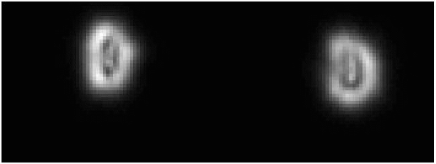
Figure 5: Pairs of defocused spots in the DIMM channel: nearly perfect spots seen with a point-source simulator in the laboratory (top) and astigmatic (about 60 nm rms) spots produced by a star and a telescope with spherical aberration (bottom) which correspond to a Strehl ratio of $\sim$0.6.

4.2.2 Optical quality

Until recently, the optical quality of the spots has not been identified as a major source of systematic errors in DIMM. A significant bias in the seeing is actually caused by the complex interaction between aberrations and scintillation, as evidenced by the study of TK07 and some experiments (Wang et al., 2006). By maintaining nearly-diffraction image quality, $S>0.6$, we avoid strong bias even for high-altitude turbulent layers.

When the MASS-DIMM system is set, the optical quality must be controlled by taking long-exposure ($\geq 30$ s) images of slightly defocused spots of some faint star under good seeing and good tracking. Atmospheric distortions are averaged out, while aberrations manifest themselves as distortions of the “donuts” (Fig. 5). The aberrations can be quantified by the donut method of Tokovinin & Heathcote (2006). This check must be repeated regularly because the telescope alignment is never very stable. Astigmatism in the direction of the baseline is acceptable in the drift-scan mode.

The defocus caused by temperature changes and mechanical instability in the telescope is usually a major contributor to the spot degradation. The MASS-DIMM instrument has no internal focusing stage, while the focusing of amateur telescopes is manual. There is no free clearance in the standard Meade fork mount for using motorised focus adaptors with MASS-DIMM and LX-200. In this respect, Meade RCX-400 with motorised focus is better.

The separation of the spots $\Delta x$ changes with telescope focus and can serve to stabilise it when the motorised focus control is available. Of course, the separation also depends on the alignment of the MD1 and MD2 mirrors, but our experience shows that it is stable enough. For a given MASS-DIMM system, the plot of Strehl ratio versus $\Delta x$ shows a broad maximum corresponding to the optimum focus.

The degradation of the Strehl ratio $S$ caused by defocus can be quantified by noting that the corresponding rms phase aberration $\sigma_{\varphi}$ is related to the change in the angular spot separation $A$,

$$S_{\rm defoc.}\approx S_{0}\exp[-\sigma_{\varphi}^{2}]=S_{0}\exp\left[-\frac{\pi^{2}}{48}\left(\frac{AD}{\lambda}\right)^{2}\left(\frac{D}{B}\right)^{2}\right].$$ (10)

The $A$ can be converted from radians to pixels if divided by the angular pixel scale. If we require $S/S_{0}>0.8$, this translates to $A<1.04(\lambda/D)(B/D)$, or about 2.6 arcsec for typical parameters $D=0.1$ m, $B/D=2.5$, $\lambda=0.5$ $\mu$m. This gives an idea of the acceptable tolerance on the spot separation. The defocus tolerance is proportional to $D^{-2}$, favouring smaller apertures, so typical $\sim$8 cm DIMM apertures are a good compromise between sensitivity and robustness.

4.2.3 Centroid noise

It follows from Eq. 8 that for a correct estimation of the noise bias, two CCD camera parameters must be known: the readout noise $R$ and the camera gain $G$. Both are measured in a standard way, by computing signal variance at different illumination levels. The readout noise can be also estimated from the data frames by calculating the background variance. Typically, the noise is small and its subtraction or not does not matter. However, the noise can significantly bias DIMM results under good seeing or for faint stars. We strongly recommend to calculate the noise variance of each spot in real time and subtract the noise contribution of both spots from the measured differential variance.

4.2.4 CCD pattern noise

Many front-illuminated CCD detectors have regular variations of the sensitivity over their pixels. Depending on a type of CCD, the sensitivity variations may be in the horizontal (as in inter-line CCDs) or vertical (as in frame transfer CCDs) directions. When size of a star image is close to Nyquist limit, such intra-pixel sensitivity variations cause errors in the centroids, depending on spot position. Thus, the common motion of the image pair in a DIMM can produce the variation of the image separation. In real measurements, common motion is normally present due to telescope vibrations, tracking errors, and turbulence.

Naturally, if the CCD has intra-pixel sensitivity variations along the lines (horizontal), the longitudinal variance will be affected only by the horizontal motion. In a chessboard-like pattern (as in colour CCDs), both horizontal and vertical motions of the spots will cause errors in both longitudinal and transverse directions.

To be sure that this effect is negligible for a chosen CCD camera, a simple test must be done with a star simulator. We move the arfificial star by few pixels during the seeing measurements. If there is no modulation, the total variance will correspond to the centroid noise (Eq. 8). Fig. 6 shows the result of such experiment with the Prosilica EC650 camera, demonstrating clearly the abscence of the pattern noise. A weak increase of the differential variance in Fig. 6 is likely explained by the large-scale sensitivity variation of the CCD and smearing of spots.

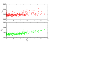
Figure 6: Dependence of measured differential variance in longitudinal ($\sigma_{\Delta x}$, top) and transverse ($\sigma_{\Delta y}$, bottom) directions on the r.m.s. amplitude of the artificial star motion (both in pixels) for the Prosilica CCD camera. The calculated centroid noise is about 0.027 pixels.

4.3 Data quality control

A working site monitor with a MASS-DIMM inevitably produces some bad data, to be discarded a posteriori by applying suitable criteria, filters. Any such filtering must not distort the statistical distribution of the measured atmospheric parameters. When the system works correctly, only a small fraction of the data is rejected.

4.3.1 DIMM data filters

The Strehl ratio $S$ is a good measure of the optical quality. However, even in a perfect DIMM $S$ is reduced under bad seeing when $r_{0}<D$. Hence, by setting a fixed threshold $S_{0}$ and rejecting data with $S<S_{0}$ we bias the seeing statistics. A more elaborate seeing-dependent threshold should be used instead (Wang et al., 2006). Alternatively, a relation between $S$ and spot separation $\Delta x$ is established empirically and the data are filtered by condition $|\Delta x-\Delta x_{0}|<A$, where $\Delta x_{0}$ is the optimum spot separation and $A$ is the acceptable half-range evaluated from (10).

4.3.2 MASS data filters

Various parameters stored in the MASS data files can be used to select valid data. The rejection thresholds are specific for each instrument, so the values given in Table 3 are only indicative.

Table 3: MASS data filters

Parameter	Rejection	Rejection reason
Flux in D-aperture $F_{D}$	$F_{D}<100$	Faint star or clouds
Flux error $\delta F_{D}$	$\delta F_{D}>0.01$	Cirrus clouds, bad guiding
Model error $\chi^{2}$	$\chi^{2}>100$	Bad profile restoration
Relative background $B_{D}/F_{D}$	$B_{D}/F_{D}>0.03$	Bright sky or star in the aperture

In addition to criteria on individual measurements, the sanity check on the data set as a whole is done by calculating average relative residuals between scintillation indices and their model (the residuals are saved). Average residual exceeding 5% on any of the indices is a strong indication of some problem such as wrong parameter settings, scattered light or vignetting. The vignetting is also monitored by the average flux ratio $F_{C}/F_{D}$ which increases when the aperture D is vignetted. The ratio depends slightly on the colours of the stars because individual PMTs have slightly different spectral response.

4.4 Reprocessing

MASS data compromised by the wrong setting of some parameters can be recovered by re-processing. For example, we can study the long-term variation of the $p$-parameters and then apply their correct values to the old data. A wrong setting of the computer clock (hence wrong air mass calculation) can be corrected, too. A set of tools for re-processing is provided together with the TURBINA program. Individual statistical moments with 1-s integration are used in the re-processing and must be archived together with the main MASS data files.

Starting from March 2006, a new algorithm for correcting the effect of strong scintillation (over-shoots) is implemented in TURBINA. All previous data must be re-processed with this new algorithm to correct over-shoots and TP distortion caused by strong scintillation. The correction method and an example of re-processing are given in TK07.

5 Examples and applications

5.1 Data examples

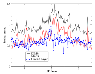
Figure 7: Data from the MASS-DIMM at Cerro Tololo, February 7/8 2007. The total seeing measured by DIMM, free-atmosphere seeing from MASS and the ground-layer seeing derived by subtraction is plotted.

Figure 7 shows a plot of the seeing measured by a MASS-DIMM site monitor at Cerro Tololo on the night of February 7/8, 2007. This night was chosen because a significant part of the turbulence was located at an altitude of $\sim 4$ km and sensed by both instruments. The spikes of seeing are perfectly correlated. When the ground-layer (GL) seeing is calculated as $J_{\rm GL}=J_{\rm DIMM}-J_{\rm MASS}$ (MASS corrected for over-shoots, $J$ defined by Eq. 1), these spikes disappear. This is a convincing demonstration of the fact that both instruments measure the seeing on the same, absolute scale. Both DIMM and MASS are calibrated independently, without any mutual adjustments or corrections.

The subtraction procedure illustrated in Fig. 7 does not work when the scintillation becomes strong, $s^{2}_{A}>0.7$ (cf. Eq. 2). Under these conditions, MASS typically over-estimates the seeing even after over-shoot correction, while DIMM under-shoots. Both instruments thus lose their accuracy under strong scintillation.

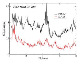
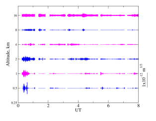
Figure 8: Data from the MASS-DIMM at Cerro Tololo, March 3/4 2007. The total seeing measured by DIMM was dominated by the ground layer, while the free-atmosphere seeing was very good (top). The turbulence profiles (bottom) show that, except for the beginning of the night, most turbulence was located in the highest 16-km layer.

Half or more of the total turbulence integral is often produced by the GL. The GL contribution can be estimated then reliably by subtraction. On some nights, the seeing in the free atmosphere is good and stable, between 0$\aas@@fstack{\prime\prime}$2 and 0$\aas@@fstack{\prime\prime}$3 (Fig. 8). These conditions, encountered infrequently but regularly at all observatories where MASS-DIMM operates, resemble Antarctic sites (e.g. Lawrence et al., 2004). If ground-layer turbulence were compensated by AO, an excellent image quality over wide field could be achieved on these calm nights. Such special conditions cannot be recognised only with a DIMM because the total seeing on these calm nights is always dominated by the GL and not at all exceptional. Such calm periods can last for several nights (e.g. Tokovinin et al., 2003b). At Cerro Pachón, the free-atmosphere seeing is better than 0$\aas@@fstack{\prime\prime}$29 during 25% of clear night time (Tokovinin & Travouillon, 2006).

5.2 Applications

5.2.1 Site testing

A possibility to monitor turbulence in the free atmosphere with a small and robust instrument such as MASS is of high value to site testing. MASS is not sensitive to small pointing errors and can work even from a heated room through a window, as demonstrated by the first night-time seeing measurements in Antarctica (Lawrence et al., 2004).

The development of the MASS-DIMM instrument has been primarily driven by the need to characterise new and existing sites for the Thirty Meter Telescope (TMT) project (Wang et al., 2006). Six MASS-DIMMs were deployed together with robotic site-testing telescopes and other equipment. The data collection is being continued. Prior to the deployment, the equipment has been extensively tested at Cerro Tololo. A European program of site selection for a large telescope will use four MASS-DIMMs. The program of Las Campanas site characterisation for the 20-m Giant Magellan Telescope uses one MASS-DIMM.

The advantage of a MASS-DIMM is obvious, as it permits to differentiate atmospheric regions where seeing is degraded, whereas a simple DIMM measures only integrated seeing. Significant differences between sites with comparable seeing caused by the GL turbulence now become apparent. Moreover, measurements of $\theta_{0}$ and $\tau_{0}$ provided by MASS are essential for selecting sites better suited for AO.

5.2.2 Site monitoring

First systematic measurements of TP at Cerro Tololo have been done with separate MASS and DIMM monitors (Tokovinin et al., 2003b). Combined MASS-DIMM site monitors based on 25-cm Meade telescopes work in robotic mode both at the Cerro Tololo and at Cerro Pachón observatories since 2004. The data from MASS are available publicly, the data from DIMMs – upon request. These openly available data are used in some studies (Kenyon et al., 2006). The statistical analysis of the MASS-DIMM data for Cerro Pachón shows a good agreement with previous data sets and leads to a new model of TP at this observatory (Tokovinin & Travouillon, 2006).

High photometric stability of the MASS detectors permits to study the atmospheric transparency and its variations (in the MASS spectral band) and to obtain photometric characterisation of a site.

5.2.3 Support of adaptive optics

Statistics of TP and $\tau_{0}$ delivered by MASS-DIMMs gives useful input for predicting performance of current and future AO systems. Britton (2006) compared the actual anisoplanatism in AO images with calculations based on simultaneous TPs from MASS-DIMM and found that the latter provide a very good diagnostic. A large collection of TPs at Cerro Pachón served to evaluate the gain from a Ground-Layer AO (GLAO) in statistical sense (Tokovinin, 2004). A similar GLAO study for Gemini (Anderson et al., 2006) is based on the TP model, while the GLAO study for the Magellan telescope used real TPs from MASS-DIMM (Athey et al., 2006).

Real-time monitoring of TP with MASS-DIMM opens a new exciting possibility to schedule critical AO observations flexibly, taking advantage of the best available conditions. These conditions are comparable to the calm atmosphere over Antarctic plateau, but are encountered at existing observatories with 10-m class telescopes and an overall seeing better than in Antarctica. Potential improvement of AO capabilities (more uniform correction in a wider field, operation at visible wavelengths) is too important to miss and gives a strong incentive for flexible AO scheduling.

To date, a total of 22 MASS-DIMM instruments have been fabricated and delivered to several observatories and programs. There are all reasons to believe that these instruments will make a significant contribution to our understanding of atmospheric turbulence and will extend the potential of new methods such as AO and interferometry. MASS-DIMM becomes a standard instrument for site testing and monitoring.

References

- Anderson et al. (2006) Andersen D.R., Stoesz J., Morris S., Lloyd-Hart M., Crampton D., Butterly T., Ellerbroek B., Jolissaint L. et al., 2006, PASP, 118, 1574
- Athey et al. (2006) Athey A., Shectman S., Phillips M., Thomas-Osip J., 2006, in Ellerbroeck B.L., Bonaccini C.D., eds., Advances in Adaptive Optics II, Proc. SPIE, 6272, 627217
- Britton (2006) Britton M. C., 2006, PASP, 118, 885
- Habib et al. (2006) Habib A., Vernin J. Benkhaldoun Z., Lanteri H., 2006, MNRAS, 368, 1456
- Hardy (1998) Hardy J.W. 1998, Adaptive Optics for Astronomical Telescopes. Oxford Univ. Press, Oxford
- Kenyon et al. (2006) Kenyon S., Lawrence J.S., Ashley M.C.B., Storey J.W.V., Tokovinin A., Fossat E., 2006, PASP, 118, 924
- Kornilov et al. (2003) Kornilov V., Tokovinin A., Voziakova O., Zaitsev A., Shatsky N., Potanin S., Sarazin M., 2003, Proc. SPIE, 4839, 837
- Lawrence et al. (2004) Lawrence J.S., Ashley M.C.B., Tokovinin A., Travouillon T., 2004, Nature, 431, 278
- Roddier (1981) Roddier F. 1981, in Wolf E., ed. Progress in Optics, Vol. 19. North-Holland, Amsterdam, p. 281
- Sarazin & Roddier (1990) Sarazin M., Roddier F., 1990, A&A, 227, 294
- Tatarskii (1961) Tatarskii V.I., 1961, Wave Propagation in a Turbulent Medium. Dover Press, New York
- Tokovinin (2002a) Tokovinin A., 2002a, PASP, 114, 1156
- Tokovinin (2002b) Tokovinin A., 2002b, Appl. Opt., 41, 957
- Tokovinin (2003) Tokovinin A., 2003, J. Opt. Soc. Am. A, 20, 686
- Tokovinin (2004) Tokovinin A., 2004, PASP, 116, 941
- Tokovinin et al. (2003a) Tokovinin A., Kornilov V., Shatsky N., Voziakova O., 2003a, MNRAS, 2003, 343, 891
- Tokovinin et al. (2003b) Tokovinin A., Baumont S., Vasquez J., 2003b, MNRAS, 340, 52
- Tokovinin et al. (2005) Tokovinin A., Vernin J., Ziad A., Chun M., 2005, PASP, 117, 395
- Tokovinin & Heathcote (2006) Tokovinin A., Heathcote S., 2006, PASP, 118, 1165
- Tokovinin & Travouillon (2006) Tokovinin A., Travouillon T., 2006, MNRAS, 365, 1235
- Tokovinin & Kornilov (2007) Tokovinin A., Kornilov V., 2007, MNRAS, accepted (TK07)
- Wang et al. (2006) Wang L., Schoeck M., Chanan G., Skidmore W., Bustos E., Seguel J., Blum R., 2006, in Stepp L.M., ed., Ground-based and Airborne Telescopes, Proc. SPIE, 6267, 62671S
- Ziad et al. (2000) Ziad A., Conan R., Tokovinin A., Martin F., Borgnino. J., 2000, Appl. Opt., 39, 5415