Dipole-dipole interaction between orthogonal dipole moments in time-dependent geometries

Abstract

In two nearby atoms, the dipole-dipole interaction can couple transitions with orthogonal dipole moments. This orthogonal coupling accounts for a number of interesting effects, but strongly depends on the geometry of the setup. Here, we discuss several setups of interest where the geometry is not fixed, such as particles in a trap or gases, by averaging over different sets of geometries. Two averaging methods are compared. In the first method, it is assumed that the internal electronic evolution is much faster than the change of geometry, whereas in the second, it is vice versa. We find that the orthogonal coupling typically survives even extensive averaging over different geometries, albeit with qualitatively different results for the two averaging methods. Typically, one- and two-dimensional averaging ranges modelling, e.g., low-dimensional gases, turn out to be the most promising model systems.

I Introduction

Two nearby atoms can interact in an energy-transfer process via the vacuum where one of the atoms is de-excited whereas the other atom is excited book-agarwal ; thiranumachandran ; book-ficek ; FiTa2002 . This dipole-dipole interaction has been studied in great detail, albeit mostly for the case of two-level atoms with parallel transition dipole moments MaKe2003 ; chang ; RuFiDa1995 ; Ja1993 ; jump ; Fi1991 ; VaAg1992 ; entanglement ; bargatin ; AgPa2001 ; pra-geometry ; breakdown ; dfs ; strong . It is known to modify the collective system dynamics and thus virtually all observables considerably, as was also shown in a number of related experiments experiment ; experiment2 ; experiment3 ; hettich ; exp-qdot ; noel ; experiment4 . Recently, it was found that a new class of effects arises from the dipole-dipole coupling between transitions with orthogonal dipole moments AgPa2001 ; pra-geometry ; breakdown ; dfs . This coupling is somewhat surprising since for single-atom systems, only near-degenerate non-orthogonal transitions can be coupled via the vacuum book-ficek . But in real atoms, e.g., transitions from one state to different Zeeman-sublevels of a different electronic state typically have orthogonal transition dipole moments. Therefore, the vacuum-coupling of such transitions in single atoms usually does not occur, which is unfortunate, since the corresponding couplings are known to give rise to many fascinating applications book-ficek .

In contrast, orthogonal transition dipole moments in different atoms do interact via the vacuum, with coupling coefficients dependent on the relative alignment of the atoms, see Fig. 1. It was shown in AgPa2001 that this interaction creates coherences involving excited states that are not driven by any laser fields. This observation can be generalized by studying the two-particle master equation under rotations of the inter-atomic distance vector breakdown . It was found that because of the orthogonal couplings, typically complete Zeeman manifolds have to be considered in modelling the dipole-dipole interaction of two atoms, such that the usual few-level approximation is no longer possible. The orthogonal couplings crucially influence the system dynamics. For example, the long-time dynamics of a two-atom system can strongly depend on the relative orientation of the two atoms pra-geometry . For a suitable laser and detector setup, undampened periodic oscillations in the fluorescence intensity are observed for some relative orientations of the two atoms, whereas the system evolves into a stationary steady state for other relative orientations. The reason for this geometry-dependence is the structure of the dipole-dipole constants. If the coupling of orthogonal transition dipole moments vanishes, then also the oscillations in the long-time limit vanish.

Figure 1: (Color online) In the left subfigure the geometry of our system is shown. The inter-atomic distance vector $\bm{r}_{12}$ is parameterized by the angles $\theta$ and $\phi$ and the length $r_{12}$. Atom A is located in the origin and atom B at $\bm{r}_{12}$. Each atom is a three-level system in $\Lambda$ configuration (b). The two lower states have an energy separation $\delta$. $\Omega_{1}$ ($\Omega_{2}$) is the Rabi frequency of the driving laser field coupling to transition $1\leftrightarrow 3$ ($2\leftrightarrow 3$) and the spontaneous decay rates are $\gamma_{1}$ and $\gamma_{2}$.

In many situations of interest, however, the geometry is not fixed. For example, in a linear trap, the inter-atomic distance usually can be described classically as a sinusoidal oscillation around a mean distance. In this case, a dependence of the dynamics on the orientation of the dipole moments relative to the oscillation direction can be expected. A gas of atoms corresponds to a setup where both the orientation and the distance of any given pair changes with time. Thus the question arises, whether the geometry-dependent effects of the dipole-dipole interaction of orthogonal transition dipole moments survive an averaging over different geometries.

Therefore, here we discuss the fluorescence intensity emitted by a pair of three-level $\Lambda$-type atoms when averaged over sets of different geometries of interest, see Fig. 1. Our primary interest is the question whether the dipole-dipole couplings of orthogonal transition dipole moments survives an averaging over different geometries and thus also is of relevance if the two atoms are not fixed in space. Since the modulations in the fluorescence intensity are a direct consequence of these couplings, they are a convenient indicator and allow for a quantitative analysis. The second major question involves the way the averaging should be treated theoretically. For comparison, we discuss two different ansatzes. First, one can assume that the internal electronic dynamics is much faster than the change of the geometrical setup. On the other hand, we consider the case where the change on geometry is fast enough such that the atoms essentially see an averaged interaction potential. The latter approach for example is used in the context of ultracold quantum gases to derive the $1/r$ long-range potential from the dipole-dipole coupling of parallel dipole moments by averaging over all possible orientations of the inter-atomic distance vectors thiranumachandran .

We find that in general the orthogonal couplings can survive an extensive averaging over different geometries as long as the inter-particle distance remains small. The magnitude of the effects in the averaged signal, however, strongly depends on the averaging range, and also on the averaging method. Typically, one- or two-dimensional systems can be expected to show larger effects of the dipole-dipole coupling. We also show that the two averaging methods considered can give very different results when averaged over the same set of geometries. In most situations, however, the case where the change in geometry is slow as compared to the internal dynamics is more favorable.

The article is organized as follows: In Sec. II.1, we present the model system, derive the equations of motion and discuss our main observable, the time-dependent fluorescence intensity. In Sec. II.2, the two averaging methods are presented and discussed. Sec. III presents the results from the averaging for various different situations of interest. Finally, our findings are discussed and summarized in Sec. IV.

II Theory

II.1 The model system

We consider a system consisting of two identical three-level atoms in $\Lambda$ configuration, see Fig. 1. The atomic states have energies $\hbar\omega_{i}$ ($i\in\{1,2,3\}$). The transition dipole moments of each individual atom are assumed perpendicular, as it is common for near-degenerate electronic states in atomic systems such as Zeeman sublevels. For simplicity, both transition dipole moments are assumed to be real; the one of the $1\!\leftrightarrow\!3$ transition $\bm{d}_{1}=(d_{1},0,0)^{T}$ is orientated along the $x$ direction and that of the $2\!\leftrightarrow\!3$ transition $\bm{d}_{2}=(0,d_{2},0)^{T}$ along the $y$ direction. A comparison with the case of complex dipole moments coupling to circularly polarized light was given in AgPa2001 . It should be noted that it was found in breakdown that in general all Zeeman sublevels of two nearby dipole-dipole interacting multilevel atoms have to be considered in order to correctly account for the different dipole-dipole couplings occurring in the system. Couplings to certain Zeeman sublevels can be eliminated, however, in special geometries, or via a detuning between the different transition frequencies, thus recovering the well-known few-level systems. In the following, we are interested in arbitrary geometries, and are thus restricted to an elimination via detunings. A $\Lambda$-type level scheme could be realized, for example, in a four-level $J\!=\!1/2\leftrightarrow J\!=\!1/2$ scheme time-energy subject to a static magnetic field, such that the energy spacing between the upper states is sufficiently large to neglect dipole-dipole coupling to one of the upper states in the four-level scheme. The frequency difference between the two lower states is denoted by $\delta$. Atom A is located in the origin of our coordinate system $\bm{r}_{1}=(0,0,0)^{T}$ and atom B at $\bm{r}_{2}=\bm{r}_{12}=r_{12}\,(\sin\theta\cos\phi,\sin\theta\sin\phi,\cos\theta)^{T}$, where the distance vector between the two atoms is $\bm{r}_{12}$. The driving laser fields propagate in $z$ direction. For this system the Hamiltonian reads

$$H=H_{a}+H_{f}+H_{vac}+H_{L}\,,$$ (1)

with

$$H_{a}= \sum_{\mu=1}^{2}\sum_{j=1}^{3}\hbar\omega_{j}\,S_{jj}^{(\mu)}\,,$$ (2a)

$$H_{f}= \sum_{\bm{k}\lambda}\hbar\omega_{k\lambda}\>a_{\bm{k}\lambda}^{\dagger}a_{\bm{k}\lambda}\,,$$ (2b)

$$H_{vac}= -\sum_{\mu=1}^{2}\left[\left(\bm{d}_{1}\,S_{31}^{(\mu)}+\bm{d}_{2}\,S_{32}^{(\mu)}\right)\bm{E}(\bm{r}_{\mu})+\textrm{H.c.}\right],$$ (2c)

$$H_{L}= -\hbar\sum_{\mu=1}^{2}\left(\Omega_{1}(\bm{r}_{\mu})e^{-i\nu_{1}t}S_{31}^{(\mu)}\right.$$

$$\left.+\Omega_{2}(\bm{r}_{\mu})e^{-i\nu_{2}t}S_{32}^{(\mu)}+\textrm{H.c.}\right)\,.$$ (2d)

$H_{a}$ represents the free energy of the atomic states. The free energy of the vacuum field is described by $H_{f}$. $H_{vac}$ is the interaction Hamiltonian of the vacuum field, and $H_{L}$ is the term describing the interaction with the laser fields in rotating-wave approximation (RWA). The laser fields have amplitudes $\mathcal{E}_{i}$, frequencies $\nu_{i}$ and polarization unit vectors $\hat{\bm{\epsilon}}_{i}$ ($i\in\{1,2\}$), respectively. $\Omega_{i}(\bm{r})=\Omega_{i}\exp[i\bm{k}_{i}\cdot\bm{r}]$ with $\Omega_{i}=(\bm{d}_{i}\cdot\hat{\bm{\epsilon}}_{i})\mathcal{E}_{i}/\hbar$ are the corresponding Rabi frequencies. $\bm{E}(\bm{r})$ represents the quantized vacuum field modes. Furthermore, $\omega_{k\lambda}$ is the frequency of a vacuum field mode with creation and annihilation operator $a_{\bm{k}\lambda}^{\dagger}$ and $a_{\bm{k}\lambda}$, respectively. The energy of the atomic state $|i\rangle$ is $\hbar\omega_{i}$. We define atomic operators

$$S_{ij}^{(k)}=|i\rangle_{k}{}_{k}\langle j|\qquad(i,j\in\{1,2,3\}\textrm{ and }k\in\{1,2\})\,,$$ (3)

where $|i\rangle_{k}$ denotes the $i$th electronic state of atom $k$. For $i\!=\!j$, Eq.(3) corresponds to a population, whereas for $i\!\neq\!j$ it is a transition operator.

Choosing a suitable interaction picture it is possible to describe the system by the master equation for the atomic density operator $\rho$ given by pra-geometry

$$\frac{\partial\rho}{\partial t}=-i\sum_{\mu=1}^{2}\sum_{j=1}^{2}\left[\Delta_{j}S_{jj}^{(\mu)},\rho\right]\allowdisplaybreaks[2]$$

$$+i\sum_{\mu=1}^{2}\sum_{j=1}^{2}\left[\left(S_{3j}^{(\mu)}\Omega_{j}(\bm{r}_{\mu})+\textrm{H.c.}\right),\rho\right]\allowdisplaybreaks[2]$$

$$-\sum_{\mu=1}^{2}\sum_{j=1}^{2}\Bigl{[}\gamma_{j}\left(S_{33}^{(\mu)}\rho-2S_{j3}^{(\mu)}\rho S_{3j}^{(\mu)}+\rho S_{33}^{(\mu)}\right)\allowdisplaybreaks[2]$$

$$+\Gamma_{j}^{dd}\left(S_{3j}^{(\mu)}S_{j3}^{(\neg\mu)}\rho-2S_{j3}^{(\neg\mu)}\rho S_{3j}^{(\mu)}+\rho S_{3j}^{(\mu)}S_{j3}^{(\neg\mu)}\right)\Bigr{]}\allowdisplaybreaks[2]$$

$$+\sum_{j=1}^{2}\left(i\Omega_{j}^{dd}\left[S_{3j}^{(1)}S_{j3}^{(2)},\rho\right]+\textrm{H.c.}\right)\allowdisplaybreaks[2]$$

$$-\sum_{\mu=1}^{2}\left[\Gamma_{vc}^{dd}\left(S_{32}^{(\mu)}S_{13}^{(\neg\mu)}\rho-2S_{13}^{(\neg\mu)}\rho S_{32}^{(\mu)}\right.\right.$$

$$\left.\left.\qquad\qquad+\rho S_{32}^{(\mu)}S_{13}^{(\neg\mu)}\right)e^{i\Delta t}+\textrm{H.c.}\right]\allowdisplaybreaks[2]$$

$$+\sum_{\mu=1}^{2}\left(i\Omega_{vc}^{dd}\left[S_{32}^{(\mu)}S_{13}^{(\neg\mu)},\rho\right]e^{i\Delta t}+\textrm{H.c.}\right)\,.$$ (4)

Here, the RWA and the Born-Markov approximation were used. The first term, which contains the detunings $\Delta_{i}=\nu_{i}-(\omega_{3}-\omega_{i})$ of the driving laser fields, appears because of the chosen interaction picture. The interaction with the laser fields is expressed by the second summand with the Rabi frequencies $\Omega_{j}(\bm{r}_{\mu})$. The contribution containing $\gamma_{j}$ represents the individual spontaneous decay of each transition in the two atoms. In our case the spontaneous decay rate on transition $3\!\leftrightarrow\!j$ is denoted as $2\gamma_{j}$. The term with $\Gamma_{j}^{dd}$ contains the dipole-dipole coupling between a dipole of one atom and the corresponding parallel dipole of the other atom. The contribution proportional to $\Omega_{j}^{dd}$ represents the corresponding dipole-dipole energy shift. The interaction between a dipole moment of one atom and the perpendicular one of the other atom is described by the expression containing the cross coupling constants $\Gamma_{vc}^{dd}$ and $\Omega_{vc}^{dd}$. The symbol $\neg\mu$ denotes the other atom than $\mu$, e.g., for $\mu=2$ one has $\neg\mu=1$. Note that the interaction picture in Eq. (4) is chosen such that the residual explicit time dependence $\exp[\pm i\Delta t]$ which cannot be transformed away is attributed to the terms that describe dipole-dipole coupling of orthogonal transition dipole moments. This choice is motivated by the physical origin of this time dependence, which arises from these orthogonal couplings pra-geometry . The frequency $\Delta$ is determined by $\Delta=\delta+\Delta_{2}-\Delta_{1}=\nu_{2}-\nu_{1}$.

The spontaneous decay rates are given by

$$\gamma_{i}=\frac{1}{4\pi\epsilon_{0}}\frac{2|\bm{d}_{i}|^{2}\omega_{3i}^{3}}{3\hbar c^{3}}\,,$$ (5)

and the dipole-dipole coupling constants can be calculated from AgPa2001

$$\Gamma_{i}^{dd} = \frac{1}{\hbar}[\bm{d}_{i}\cdot\textrm{Im}(\overset{\leftrightarrow}{\chi})\cdot\bm{d}_{i}^{*}]\,,$$ (6a)

$$\Omega_{i}^{dd} = \frac{1}{\hbar}[\bm{d}_{i}\cdot\textrm{Re}(\overset{\leftrightarrow}{\chi})\cdot\bm{d}_{i}^{*}]\,,$$ (6b)

$$\Gamma_{vc}^{dd} = \frac{1}{\hbar}[\bm{d}_{2}\cdot\textrm{Im}(\overset{\leftrightarrow}{\chi})\cdot\bm{d}_{1}^{*}]\,,$$ (6c)

$$\Omega_{vc}^{dd} = \frac{1}{\hbar}[\bm{d}_{2}\cdot\textrm{Re}(\overset{\leftrightarrow}{\chi})\cdot\bm{d}_{1}^{*}]\,.$$ (6d)

In evaluating these coupling constants we have approximated $\omega_{31}\approx\omega_{32}\approx\omega_{0}$. Re and Im denote the real and imaginary part of the tensor $\overset{\leftrightarrow}{\chi}$ whose components are given by

$$\chi_{\mu\nu} (\bm{r}_{1},\bm{r}_{2})=\frac{1}{4\pi\epsilon_{0}}\left[\delta_{\mu\nu}\left(\frac{k_{0}^{2}}{r_{12}}+\frac{ik_{0}}{r_{12}^{2}}-\frac{1}{r_{12}^{3}}\right)\right.-$$

$$\left.\frac{(\bm{r}_{12})_{\mu}(\bm{r}_{12})_{\nu}}{r_{12}^{2}}\left(\frac{k_{0}^{2}}{r_{12}}+\frac{3ik_{0}}{r_{12}^{2}}-\frac{3}{r_{12}^{3}}\right)\right]\,e^{ik_{0}r_{12}}\,.$$ (7)

$\delta_{\mu\nu}$ is the Kronecker delta symbol. For our choice of the atomic system, the coupling constants between orthogonal dipole moments evaluate to ($\eta=k_{0}\,r_{12}$)

$$\Gamma_{vc}^{dd} =-\frac{3}{4}\,\sqrt{\gamma_{1}\gamma_{2}}\,\sin(2\phi)\,\sin^{2}\theta$$

$$\qquad\times\left[\frac{\sin\eta}{\eta}+3\left(\frac{\cos\eta}{\eta^{2}}-\frac{\sin\eta}{\eta^{3}}\right)\right]\,,$$ (8a)

$$\Omega_{vc}^{dd} =-\frac{3}{4}\,\sqrt{\gamma_{1}\gamma_{2}}\,\sin(2\phi)\,\sin^{2}\theta$$

$$\qquad\times\left[\frac{\cos\eta}{\eta}-3\left(\frac{\sin\eta}{\eta^{2}}+\frac{\cos\eta}{\eta^{3}}\right)\right]\,.$$ (8b)

Our main observable is the total time-dependent fluorescence intensity emitted by the two atoms. It is assumed to be measured by a detector placed on the $y$-axis at the point $\bm{R}=R\hat{\bm{R}}$ with $\hat{\bm{R}}=(0,1,0)^{T}$. This intensity is proportional to the normally ordered one-time correlation function

$$I=\langle\,:\!\bm{E}^{(-)}(\bm{R},t)\>\bm{E}^{(+)}(\bm{R},t)\!:\,\rangle\,,$$ (9)

where $\bm{E}^{(\mp)}(\bm{x},t)$ are the positive and negative frequency parts of the vacuum field $\bm{E}(\bm{x},t)=\bm{E}^{(-)}(\bm{x},t)+\bm{E}^{(+)}(\bm{x},t)$. For our arrangement of the detector, the atoms and the laser fields the fluorescence intensity reduces to pra-geometry

$$I_{y}=w_{1}^{2}\sum_{\mu,\nu=1}^{2}\left\langle S_{31}^{(\mu)}S_{13}^{(\nu)}\right\rangle\>e^{ik_{1}\hat{\bm{R}}\cdot\bm{r}_{\mu\nu}}\,,$$ (10)

where $w_{1}=(\omega_{31}^{2}\,d_{1})/(4\pi\epsilon_{0}c^{2}R)$ is a pre-factor that we neglect in the following.

II.2 Averaging over different geometries

The master equation Eq. (4) contains an explicit time dependence which is determined by the two driving laser field frequencies. Thus, in general, it cannot be expected that the system reaches a stationary steady state. This was demonstrated in pra-geometry , where it was shown that for $\Delta\neq 0$ in general it depends on the relative alignment of the two atoms whether the system reaches a stationary state or not. For some geometries, the long-time limit is constant, whereas for other geometries a periodic oscillation in the fluorescence intensity is predicted. Since the relative positions of nearby atoms in many experimental situations of relevance are not fixed, the question arises whether any time dependence survives when averaging over a set of geometries. The most obvious example for this is a three-dimensional volume of gas, where arbitrary relative orientations and distances can be observed. But also other sets of geometries may be considered. For example, in noel , an essentially one-dimensional ultracold quantum gas was studied. In this case, an external static field can be used to vary the relative alignment of dipoles and the trap axis.

In the following, we discuss two different approaches for calculating the averaged total fluorescence intensity, which is our main observable.

II.2.1 The adiabatic case method

In general, we have to average over the angles $\theta,\phi$ as well as over the distance $r_{12}$. We discretize the respective interval of each geometric parameter in $N_{i}$ equal steps of size $\Delta_{i}$, respectively, where $i\in\{r,\theta,\phi\}$. This gives rise to $N_{r}N_{\phi}N_{\theta}$ different geometries. For each of these geometries, we evaluate the coupling constants and numerically integrate the master equation Eq. (4). From this, we obtain the time-dependent fluorescence intensity $\left[I_{y}(t)\right]_{n_{r},n_{\theta},n_{\phi}}$ for this particular geometry $(n_{i}\in\{1,\dots,N_{i}\})$. Finally, we average over all time evolutions of the different geometries using the expression

$$\overline{\left(I_{y}\right)}(t) =\frac{1}{\mathcal{Q}}\sum_{n_{r}=1}^{N_{r}}\sum_{n_{\theta}=1}^{N_{\theta}}\sum_{n_{\phi}=1}^{N_{\phi}}\>\mathcal{V}_{r,\theta,\phi}\>\left[I_{y}(t)\right]_{n_{r},n_{\theta},n_{\phi}}\,,$$ (11a)

$$\mathcal{Q} =\sum_{n_{r}=1}^{N_{r}}\sum_{n_{\theta}=1}^{N_{\theta}}\sum_{n_{\phi}=1}^{N_{\phi}}\>\mathcal{V}_{r,\theta,\phi}\,,$$ (11b)

$$\mathcal{V}_{r,\theta,\phi} =\Delta V_{r}\>\Delta V_{\theta}(n_{r})\>\Delta V_{\phi}(n_{r},n_{\theta})\,.$$ (11c)

$\mathcal{Q}$ is a normalization constant. We work in a spherical coordinate system and do not only consider uniform motions of the atoms. Thus an appropriate volume element $\mathcal{V}_{r,\theta,\phi}$ has to be considered. In the discretized form, the contributions from the different coordinates are given by

$$\Delta V_{r} =\Delta_{r}\,,$$ (12a)

$$\Delta V_{\theta}(n_{r}) =r_{n_{r}}\Delta_{\theta}\,,$$ (12b)

$$\Delta V_{\phi}(n_{r},n_{\theta}) =r_{n_{r}}\sin(\theta_{n_{\theta}})\Delta_{\phi}\,.$$ (12c)

When we average over one or two parameters only we omit the other summation(s) and volume element(s).

This method of averaging describes the experimentally observable signal as long as the change of the geometric setup is slow compared to the internal dynamics of the system. Then, the internal dynamics adapts to its long-time evolution on a timescale much faster than the change of the geometry.

In the following, we will call this way of averaging the adiabatic case (AC) method because of the slow change of the geometry.

II.2.2 The average potential method

In our second method of averaging, a different physical situation is considered. Here, the change of the geometry is considered fast compared to the internal dynamics. Then, the time evolution of the atomic system according to the master equation Eq. (4) is not governed by coupling constants corresponding to a particular fixed geometry. Rather, the atom experiences an averaged coupling constant. Therefore, in this case, we start by averaging all coupling constants Eqs. (6) over the range of geometries considered. This can be done analytically without a discretization of the averaging range, but again taking into account an appropriate volume element. Then the averaged coupling constants are given by

$$\overline{\mathcal{C}}=\int_{0}^{2\pi}\int_{0}^{\pi}\int_{0}^{2\pi}\>\mathcal{C}\>dV_{r}\,dV_{\theta}\,dV_{\phi}\,,$$ (13)

with $\mathcal{C}\in\left\{\Gamma_{i}^{dd},\Omega_{i}^{dd},\Gamma_{vc}^{dd},\Omega_{vc}^{dd}\right\}$. In order to average, e.g., over a sinusoidally oscillating distance we parameterize $r_{12}=r_{m}+r_{a}\sin\alpha$ by a mean distance $r_{m}$ and an oscillation amplitude $r_{a}$. In this case $dV_{r}=d\alpha$, $dV_{\theta}=r_{12}d\theta$ and $dV_{\phi}=r_{12}\sin\theta d\phi$. Then, the master equation is solved and the fluorescence intensity is calculated using these averaged coupling constants. Finally, the time-dependent intensity is plugged into Eq. (10). Since the expression for the fluorescence intensity Eq. (10) also depends on the orientation of the inter-atomic distance vector, we also average this expression over the same set of geometries.

In the following, this way of averaging will be referred to as averaged potential (AP) method.

III Results

We now turn to a numerical study of our system as outlined in the previous section. Different ranges of averaging will be considered, according to different setups of interest. In all cases, the two ways of averaging the fluorescence intensity will be compared. We choose as initial condition both atoms to be in state $|3\rangle$ unless noted otherwise.

Figure 2: (Color online) Time dependence of the fluorescence intensity averaged over $r_{12}$ by the AC method. $r_{m}=0.25\lambda$ and (a) $r_{a}=0.02\lambda$, (b) $r_{a}=0.14\lambda$ and (c) $r_{a}=0.2\lambda$. The inter-atomic distance vector is oriented such that $\phi=\pi/4$ and $\theta=\pi/2$. The laser parameters are $\Omega_{1}=3\,\gamma$, $\Omega_{2}=5\,\gamma$, $\Delta_{1}=0$, $\Delta_{2}=2\gamma$, and the two lower states are assumed degenerate $\delta=0$.

Figure 3: (Color online) Dependence of the amplitude of the oscillating fluorescence intensity on the oscillation amplitude $r_{12}$ of the atom for (a) $r_{m}=0.2\lambda$ and (b) $r_{m}=0.25\lambda$. The other parameters are as in Fig. 2.

III.1 Averaging over inter-particle distance

In this section, the orientation of the inter-atomic distance vector is fixed, while we assume a sinusoidal oscillation of the distance $r_{12}$ around a mean distance $r_{m}$ with amplitude $r_{a}$, i.e., $r_{12}(\alpha)=r_{m}+r_{a}\,\sin(\alpha)$ with $\alpha\in[0,2\pi]$. This corresponds to, e.g., atoms in a linear trap. In Fig. 2, we choose a mean distance $r_{m}=0.25\lambda$ and orientation $\theta=\pi/2$, $\phi=\pi/4$. The different curves correspond to oscillation amplitudes $0.02\lambda$, $0.14\lambda$ and $0.2\lambda$, respectively. All curves in this figure were obtained using the AC method. It can be seen that in the averaged signal, the system does not reach a steady state in the long-time limit for any of these oscillation amplitudes. To analyze the oscillations in the long-time evolution in more detail, we determine the maximum (minimum) fluorescence intensity $I_{\textrm{max}}$ ($I_{\textrm{min}}$) in the long-time limit where the intensity undergoes periodic changes. We define an oscillation amplitude of the intensity as $\Delta I=I_{\textrm{max}}-I_{\textrm{min}}$. From Fig. 2, it is clear that $\Delta I$ depends on the oscillation amplitude $r_{a}$. This dependence is depicted in Fig. 3 for small mean distances $r_{m}$, where it can be seen that $\Delta I$ exhibits a resonance in the plot versus the oscillation amplitude $r_{a}$. This resonance can be understood as follows. First, one has to note that as long as the inter-atomic distance is not too small, typically the oscillation amplitude decreases with increasing particle distance, because the coupling constants between orthogonal dipole moments decrease. Therefore, small inter-atomic distances lead to a larger oscillation amplitude. Only for very small distances, the oscillation amplitude as well as the total fluorescence signal are attenuated because the dipole-dipole energy shifts move the atomic transitions out of resonance with the driving laser field, such that the upper state population is decreased. This explains why the averaged oscillation amplitude decreases from the resonance maximum towards smaller oscillation amplitude $r_{a}$. With smaller $r_{a}$, only larger inter-atomic distances are considered in the averaging, and thus the average oscillation amplitude decreases.

Figure 4: (Color online) Time-dependent fluorescence signal for different fixed distances $r_{12}$ without any averaging. (a) $r_{12}=0.10\,\lambda$, (b) $r_{12}=0.08\,\lambda$, (c) $r_{12}=0.06\,\lambda$, (d) $r_{12}=0.05\,\lambda$, (e) $r_{12}=0.04\,\lambda$. The other parameters are as in Fig. 2. The vertical lines allow to easily judge the relative phase shifts of the different curves.

The decrease of the oscillation amplitude $\Delta I$ from the resonance towards higher amplitudes is due to a different mechanism. In Fig. 3, for both mean distances $r_{m}$, this occurs if $r_{a}$ is large enough such that inter-atomic distances below about $0.06\,\lambda$ are included in the averaging. Some examples of unaveraged time-dependent signals for different inter-atomic distances are shown in Fig. 4. For distances larger than about $0.06\,\lambda$, the relevant contributions oscillate approximately in phase, see curves (a) and (b) in Fig. 4. For smaller distances, however, the contributions move out of phase, as can be seen from curves (c)-(e). Curves (d) and (e) approximately have maxima where curves (a) and (b) have minima, and vice versa. Curve (c) is an intermediate case. Therefore, the oscillations with different phases cancel each other in the averaging process if distances below about $0.06\,\lambda$ are included in the averaging.

In Fig. 5(a) we show $\Delta I$ in dependence of $r_{a}$ for a larger mean distance $r_{m}=2.25\lambda$, and over a broader range of oscillation amplitudes. It can be seen that the curve exhibits a series of resonances similar to the one shown in Fig. 3. These again occur due to an alternating destructive and constructive superposition of the different oscillations in the averaging process. The overall amplitude $\Delta I$, however, is small because of the overall larger inter-atomic distances considered in this figure.

Figure 5: (Color online) Dependence of the amplitude of the oscillating fluorescence intensity on the oscillation amplitude $r_{12}$ of the atom for larger mean distance $r_{m}=2.25\lambda$. In (a) we used the AC and in (b) the AP method. The other parameters are as in Fig. 2.

Figure 6: (Color online) Comparison of the time dependence of the fluorescence averaged over r by both methods. The orientation angles $\theta=0.5\pi$ and $\phi=0.25\pi$ are fix and $r_{m}=0.25\lambda$. (a) AC method, $r_{a}=0.14\lambda$, (b) AP method, $r_{a}=0.14\lambda$, (c) AC method, $r_{a}=0.2\lambda$, (d) AP method, $r_{a}=0.2\lambda$. All other parameters are as in Fig. 2.

Finally, we discuss the time-averaged intensity obtained from the AP method of averaging. Some examples are shown in Fig. 6. Curves (a) and (c) show our results from the AC method and (b) and (d) those from the AP method. The oscillation amplitudes are $r_{a}=0.14\lambda$ and $0.2\lambda$, respectively. All other parameters are as in Fig. 2. The left panel shows values for $5\leq\gamma\cdot t\leq 25$ since the stationary oscillation is reached rapidly for these parameters. Also in the AP case, the fluorescence intensity undergoes periodic changes in the long-time limit, see Fig. 6. For small oscillation amplitudes $r_{a}$ there is little difference between the two methods, see curves (a) and (b). However, for larger values of $r_{a}$ the amplitude of the oscillations in the AP case is much larger than those obtained in the AC averaging. The dependence of the oscillation amplitude on the averaging range for the AP method is

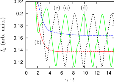
Figure 7: Time dependence of the fluorescence averaged over $\theta$ by using the AC method. The distance $r_{12}=0.1\lambda$ is fixed. (a) $\phi=0.2\pi$, (b) $\phi=0.5\pi$, (c) $\phi=0.8\pi$ and (d) $\phi=\pi$. All other parameters are as in Fig. 2.

shown in Fig. 5, curve (b). As in the corresponding curve (a) for the AC averaging method, resonance structures appear. But depending on $r_{a}$, the two methods yield either similar or very different oscillation amplitudes. In addition, the result for the AP method seems to have a root at about $r_{a}=0.4\lambda$. A careful analysis shows, however, that this minimum is not a true root. The reason for the minima in the AP curve is that for these oscillation amplitudes, the turning point at minimum inter-atomic distance is close to a distance where the coupling constants between orthogonal transition dipole moments are small. Then, the averaged coupling constants are small such that the oscillation amplitude has a minimum. These minima nicely show a crucial difference between the two averaging methods. In the AP method, it is easy to find averaging ranges where the averaged coupling constants are small or even vanish. Then, also the oscillation in the long-time dynamics is negligible. The results from the AC method, however, typically remain oscillatory even for such averaging ranges, as the dynamics for each of the different geometries contributes rather than only an averaged geometry. We will find this difference again in the following sections.

III.2 Averaging over relative orientation

In the following, we consider the case where the inter-atomic distance $r_{12}$ is fixed, but the relative orientation and thus the angles $\theta$ and/or $\phi$ are averaged over. A realization for this could be a Mexican-hat-like potential where one of the atoms is placed in a potential dip in the center whereas the other atom is confined to the potential minimum in the rim. First we fix the angle $\phi$ and assume atom B to move around A on a circle in a plane which is perpendicular to the x-y-plane and includes the origin. Since $\theta$ is only defined between $0$ and $\pi$ we have to average over two semicircles with $\phi$ and $\phi+\pi$ to include the whole circle. Some examples of our results for $r_{12}=0.1\lambda$ using the AC method of averaging are shown in Fig. 7. Here, the angle $\phi$ is chosen as $0.2\pi$, $0.5\pi$, $0.8\pi$ and $\pi$, respectively. For $\phi=0.5\pi$ and for $\phi=\pi$ the system reaches a time-independent steady state in the long-time limit. That is because the cross-coupling constants are zero for these values of $\phi$, as both $\Gamma_{vc}^{dd}$ and $\Omega_{vc}^{dd}$ are proportional to $\sin(2\phi)\sin^{2}(\theta)$, see Eqs. (8). But even though the coupling constants are zero in both cases, the resulting intensities are not identical. This demonstrates that it is not sufficient to analyze the coupling constants alone to understand the system dynamics.

Figure 8: (Color online) Time dependence of the fluorescence intensity averaged over $\theta$ with fixed inter-atomic distance $r_{12}=0.1\lambda$. (a) AC method with $\phi=0.6\pi$, (b) AP method with $\phi=0.6\pi$, (c) AC method with $\phi=0.9\pi$, and (d) AP method with $\phi=0.9\pi$. The other parameters are as in Fig. 2.

In addition we can see from Fig. 7 that there is a phase shift of $\pi$ with respect to the oscillation in the long-time limit between the two curves for $\phi=0.2\pi$ and $\phi=0.8\pi$. We found that in general curves for different values of $\phi$ split into two groups separated by such a phase shift of $\pi$. The first group contains curves for $0<\phi<\pi/2$, whereas the other consists of curves for $\pi/2<\phi<\pi$. Within each of these groups, the oscillation amplitude of the intensity has the same dependence on the angle $\phi$. For $\phi=0$ and $\phi=\pi/2$ the amplitude is zero. Then it increases with growing $\phi$ and reaches a maximum for $\phi=0.2\pi$ and $\phi=0.8\pi$, respectively. Thus, in Fig. 7 the curves with maximum oscillation amplitude are shown. This separation is likely to appear due to the change of sign of the cross-coupling constants at $\phi=0.5\pi$. This can be understood from the explicit expressions of the coupling constants Eqs. (8). In the master equation (4) we can see that a sign change in the terms with the cross-couplings can be rewritten as a constant phase shift factor of $\exp[i\pi]$. It is, however, not straightforward to connect this phase shift to the phase shift seen in Fig. 7, because the oscillation frequency of the time-dependent fluorescence in general does not only depend on $\Delta$, but also, e.g., on the laser field Rabi frequencies. In addition, one has to note that the geometric parameters $\theta,\phi$ enter the total fluorescence intensity as well, see Eq. (10). But our interpretation is further supported by the fact that a change of the inter-atomic distance $r_{12}$ has no influence on the separation of our curves into two groups. The separation also persists for different initial conditions, e.g., atom A in state $|1\rangle$ and atom B in $|3\rangle$, and thus is not a consequence of the initial dynamics until the steady state has been reached.

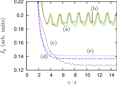
Figure 9: (Color online) Time dependence of the fluorescence intensity averaged over $\phi$. $r_{12}$ is fixed at $0.1\lambda$. (a) $\theta=0.25\pi$, (b) $\theta=0.3\pi$, (c) $\theta=0.5\pi$ and (d) $\theta=\pi$. Curves (a-d) are obtained using the AC method. (e) shows a result using the AP method for $\theta=0.3\pi$. All other parameters are as in Fig. 2.

Using the AP method the separation into two groups remains, but again the curves are different from our results from the other averaging method. In Fig. 8 we compare curves from both methods of averaging for averaging over $\theta$ with fixed angles $\phi=0.6\pi$ and $\phi=0.9\pi$. The curves resulting from the AP method have pronounced local extrema in each oscillation period in addition to the global ones, and the overall intensity is higher as in the AC case.

Next we assume atom B to move on a circle in the x-y-plane. Thus $\theta$ is fixed and we average over the angle $\phi$. The inter-atomic distance is $0.1\lambda$. Some examples of our results are shown in Fig. 9, where $\theta$ is chosen as $0.25\pi$, $0.3\pi$, $0.5\pi$ and $\pi$. For the AC method the system does not reach a time-independent state in the long-time limit except for the angle $\theta=\pi$. This is because for this choice of $\theta=\pi$ the coupling constants vanish since they are proportional to $\sin(2\phi)\sin^{2}(\theta)$, see Eqs. (8). For any different $\theta$ our system remains oscillating in the long-time limit. In case of $\theta=0.3\pi$ one can see local extrema in addition to the global extrema in the fluorescence intensity. In both cases, even the time-averaged average intensity is considerably larger than in the non-oscillatory case $\theta=\pi$. Interestingly, for $\theta=\pi/2$, the absolute value of the intensity is lower than for the non-oscillatory case $\theta=\pi$. Thus, the orthogonal coupling together with the averaging can have both an enhancing or a detrimental effect to the total emitted fluorescence.

For this set of geometries, the AP method of averaging always yields a stationary long-time limit and thus behaves qualitatively different from the first method. The reason for this is that the coupling constants for the orthogonal couplings vanish upon averaging over then angle $\phi$. As discussed before, then the time dependence in the long-time limit also vanishes, see Fig. 9.

We now turn to the case of atom B moving around A on a sphere with radius $r_{12}$. In this case, neither of the two angles $\theta$ and $\phi$ is fixed, and we have to average over both of them while the inter-atomic

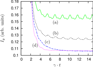
Figure 10: (Color online) Time dependence of the total fluorescence intensity averaged over $\theta$ and $\phi$ for the inter-atomic distances (a) $r_{12}=0.1\lambda$, (b) $r_{12}=0.15\lambda$ and (c) $r_{12}=0.2\lambda$. Curves (a-c) are obtained using the AC method. (d) is the result from the AP method for $r_{12}=0.1\lambda$. The other parameters are as in Fig. 2.

distance is fixed. Some results from both methods are shown in Fig. 10. We already know that the coupling constants vanish when averaged over $\phi$. That is why the time dependence in the AP method also vanishes when we average over $\theta$ and $\phi$, see curve (d). In curves (a)-(c) obtained using the AC method, the inter-atomic distance is chosen as $0.1\lambda$, $0.15\lambda$ and $0.2\lambda$, respectively. One can see that both the oscillation amplitude and the absolute value of the fluorescence intensity decrease with increasing inter-particle distance. For the distance $0.2\lambda$ there is almost no oscillation left due to the vanishing of the coupling constants with increasing inter-atomic distance. This also explains why this curve approaches the AP method result, where the averaged coupling constants are zero. As compared to curves (a) and (b) in Fig. 9, curve (a) in Fig. 10 shows that the additional averaging over $\theta$ does lead to a reduction of the oscillation amplitude. Still, the oscillation and thus the dipole-dipole coupling of orthogonal dipole moments can survive an averaging over all orientations, depending on the averaging case.

III.3 Averaging over distance and orientation

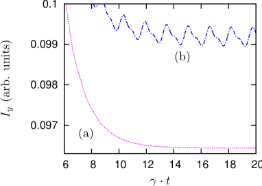
Figure 11: (Color online) Time dependence of the total fluorescence intensity averaged over r, $\theta$ and $\phi$ for atom B moving on a sphere around atom A with additional harmonic oscillation of the inter-atomic distance. Here, $r_{m}=0.2\lambda$ and $r_{a}=0.12\lambda$. In (a) we used the AP and in (b) the AC method. All other parameters are as in Fig. 2.

After the individual averaging over the inter-atomic distance and the relative orientation of the two atoms in the previous sections, we now consider the case of averaging over both. This situation is realized, e.g., in a gas of atoms, where the relative position of any two particles changes with time. An averaging over the two-particle configuration space is meaningful, since in a macroscopic volume of gas at any time there is a finite probability for an arbitrary geometry within the volume of the sample to be present. A different realization is a sample of atoms randomly embedded in a host material. In this case, again an averaging is in order. The two situations differ, however, since the former case corresponds to a time-dependent geometry for any two-particle subsystem, whereas the latter case can be represented by a sample of time-independent pairs.

Thus, in the following, we investigate whether in these cases any time dependence of the fluorescence intensity remains in the long-time limit by considering a system where $r_{12}$, $\theta$ and $\phi$ are variable. The three-dimensional case of course leaves several possibilities for the averaging range. In the following, we will consider two cases. In the first case, atom B moves on a sphere with atom A in its center and additionally oscillates around the mean distance $\bm{r}_{12}$ with an amplitude $r_{a}$. In the second case, the particle fly-by, particle B passes atom A moving with constant velocity on a straight line, see Fig. 12.

In Sec. III.2 we have seen that averaging the coupling constants over $\phi$ makes them vanish, such that the system does not show any time dependence in the long-time limit when we use the AP method of averaging. This, of course also holds true for the three-dimensional averaging for atom B moving on a sphere with oscillation of the inter-atomic distance. In contrast, the AC method of averaging still yields time-dependent fluorescence intensities. An example is shown in Fig. 11. Here, the inter-atomic mean distance is chosen $r_{m}=0.2\lambda$ and the oscillation amplitude is $r_{a}=0.12\lambda$. We see that even if we average over all three geometric parameters, the system does not reach a time-independent state in the long-time limit, even though the oscillation amplitude is small.

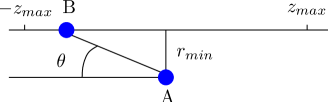
Figure 12: (Color online) Geometry for the case of atom B flying past atom A with constant velocity on a straight line from $-z_{max}$ to $z_{max}$.

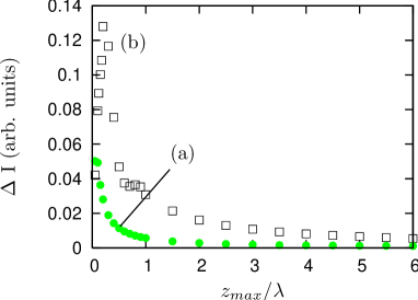
Figure 13: (Color online) Dependence of the oscillation amplitude of the time-dependent intensity on $z_{max}$ for impact parameter $r_{min}=0.05\lambda$. $\phi=\pi/4$, and the other parameters are as in Fig. 2. In (a) we used the AC and in (b) the AP method.

Finally, we consider the case where atom A flys past atom B along the z-axis from $-z_{max}$ to $z_{max}$ with constant velocity, see Fig 12. The angle $\phi$ is fixed and we average over $\theta$ and $r_{12}$ considering the respective volume element. We analyzed the case $\phi=\pi/4$ and found that for both averaging methods the fluorescence intensity remains oscillatory in the long-time limit. To further study these oscillations, in Fig. 13 we show the oscillation amplitude of the time-dependent fluorescence intensity in the long-time limit against the extend of the motion $z_{max}$. The minimum inter-atomic distance is chosen as $r_{min}=0.05\lambda$. Curve (a) shows our results from the AP and (b) those from the AC method of averaging. One can see that in both cases the amplitude decreases with increasing $z_{max}$ for large values of $z_{max}$. This is because for large distances the dipole-dipole interaction tends to zero, and oscillations only occur if the particles are close. If the averaging interval contains increasing ranges of $z$ where there essentially is no oscillation because of the inter-atomic distance, then the oscillations in the overall signal decrease. It is interesting to note, however, that in this averaging configuration the AP method shown in curve (a) yields much larger oscillations than the AC method shown in curve (b). Also, it can be seen that the AP method shows oscillations over a range of $z_{max}$ up to several wavelengths $\lambda$. The reason for this is as follows. In the AP method, the coupling constants are averaged over the different geometries. For $z=0$, the distance between the particles is $r_{min}=0.05\lambda$. At this position, the coupling constant $\Omega_{vc}^{dd}$ acquires a large value of more than $330\gamma$. Of course, with increasing distance the constant $\Omega_{vc}^{dd}$ rapidly decreases down to zero. But averaging over a certain range $[-z_{max},z_{max}]$ still gives a considerable averaged coupling constant $\bar{\Omega}_{vc}^{dd}$ even for values of $z_{max}$ where the unaveraged coupling constants are negligible. This is the reason why the oscillations persist for large $z_{max}$ values in the AP case. In contrast, in the AC case, contributions from larger $z$ values do not oscillate at all such that the decrease of the oscillation amplitude with $z_{max}$ is much more rapid.

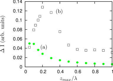
Figure 14: (Color online) Dependence of the oscillation amplitude of the time-dependent intensity on $z_{max}$ for smaller values of $z_{max}$. (a) AC method with $r_{min}=0.05\lambda$, (b) AP method with $r_{min}=0.05\lambda$. All other parameters are as in Fig. 13.

We now focus on the region with smaller motion extends $z_{max}$. The corresponding results are shown in Fig. 14 for $r_{min}=0.05\lambda$. In the limit $z_{max}\to 0$, the time-dependent fluorescence approaches the unaveraged curves (d) and (e) in Fig. 4, which exhibit relatively low oscillation amplitudes. The reason is that at this small distance, the atomic states are shifted by the dipole-dipole interaction out of resonance with the laser fields, such that the overall fluorescence is low. For both methods, the intensity oscillations first strongly enhance with increasing $z_{max}$, and then decrease again after passing through a maximum oscillation amplitude. The AC method results for larger $z_{max}$ essentially remain structureless. The AP results, however, exhibit some oscillations, and only then start to decay monotonously with increasing averaging range. Due to the complexity of the system, it is difficult to definitively attribute the oscillation to a property of the system. We believe, however, that they are due to a similar alternating constructive and destructive interference in the averaging as the one that led to the resonance structures in Figs. 3 and 5. Such resonances do not appear in the AC method results, because there the contributions for higher values of $z$ where the oscillations in the AP method appear are already too small.

IV Discussion and summary

Dipole-dipole interactions between transitions with orthogonal transition dipole moments gives rise to a new class of effects in collective quantum systems. These couplings, however, strongly depend on the geometry of the setup, and even vanish for some geometries. Therefore here we have discussed different averaging schemes to answer the question whether measurable effects of the dipole-dipole coupling of orthogonal dipole moments survive if the geometry of the system under study is not fixed. As observable, we chose the easily accessible fluorescence intensity of a pair of laser-driven $\Lambda$-type atoms, which for suitable laser parameters is known to exhibit periodic oscillations in the long-time limit due to the orthogonal couplings.

As a main result, we found that the effects of the dipole-dipole coupling of orthogonal transition dipole moments can survive extensive averaging over all three spatial dimensions. We have analyzed the obtained averaged signals, and expect our physical interpretations to carry over to other atomic level structures. Depending on the averaging range, both constructive and destructive superpositions of the contributions for the respective geometries is possible, such that a wide range of results was observed. The results also strongly depend on the method of averaging, and thus on the physical situation considered. Typically, the adiabatic case, where the geometry changes slowly as compared to the internal dynamics, is more favorable since it better preserves the intensity oscillations. In the average potential case, where the change of geometry is so fast that the atoms effectively see a dipole-dipole interaction averaged over the different geometries, some averaging ranges lead to an exact vanishing of the coupling constants. This usually does not occur in the adiabatic case. A somewhat different situation was found in the particle fly-by, where the averaging over the coupling constants in the AP method led to a much wider range of distances over which an effect of the orthogonal couplings can be observed. In general, our results show that the most pronounced effects of the orthogonal couplings in systems with variable geometry can be expected in one- or two-dimensional setups. There, it is easier to avoid detrimental averaging over extended sets of geometries, and additional control parameters such as the orientation of the dipole moments with respect to the axis of a one-dimensional sample allow to study the system properties in more detail.

References

- (1) G. S. Agarwal, in Quantum Statistical Theories of Spontaneous Emission and Their Relation to Other Approaches, edited by G. Höhler (Springer, Berlin, 1974).
- (2) D. P. Craig and T. Thirunamachandran, Molecular Quantum Electrodynamics, Academic, New York, 1984.
- (3) Z. Ficek and S. Swain, Quantum Interference and Coherence: Theory and Experiments, Springer, Berlin, 2004.
- (4) Z. Ficek and R. Tanas, Phys. Rep. 372, 369 (2002).
- (5) M. Lewenstein and J. Javanainen, Phys. Rev. Lett. 59, 1289 (1987); A. Beige and G. C. Hegerfeldt, Phys. Rev. A 59, 2385 (1999).
- (6) Z. Ficek, Phys. Rev. A 44, 7759 (1991).
- (7) G. V. Varada and G. S. Agarwal, Phys. Rev. A 45, 6721 (1992).
- (8) D. F. V. James, Phys. Rev. A 47, 1336 (1993).
- (9) T. G. Rudolph, Z. Ficek, and B. J. Dalton, Phys. Rev. A 52, 636 (1995).
- (10) I. V. Bargatin, B. A. Grishanin, and V. N. Zadkov, Phys. Rev. A 61, 052305 (2000).
- (11) M. D. Lukin and P. R. Hemmer, Phys. Rev. Lett. 84, 2818 (2000); G.-x. Li, K. Allaart, and D. Lenstra, Phys. Rev. A 69, 055802 (2004).
- (12) M. Macovei and C. H. Keitel, Phys. Rev. Lett. 91, 123601 (2003).
- (13) J.-T. Chang, J. Evers, M. O. Scully and M. S. Zubairy, Phys. Rev. A 73, 031803(R) (2006); J.-T. Chang, J. Evers and M. S. Zubairy, ibid. 74, 043820 (2006).
- (14) G. S. Agarwal and A. K. Patnaik, Phys. Rev. A 63, 043805 (2001).
- (15) J. Evers, M. Kiffner, M. Macovei and C. H. Keitel, Phys. Rev. A 73, 023804 (2006).
- (16) M. Kiffner, J. Evers and C. H. Keitel, Phys. Rev. A 76, 013807 (2007).
- (17) M. Kiffner, J. Evers and C. H. Keitel, Phys. Rev. A 75, 032313 (2007).
- (18) M. Macovei, J. Evers, G.-x. Li, and C. H. Keitel, Phys. Rev. Lett. 98, 043602 (2007).
- (19) R. G. DeVoe and R. G. Brewer, Phys. Rev. Lett. 76, 2049 (1996).
- (20) P. Mataloni, E. DeAngelis, and F. DeMartini, Phys. Rev. Lett. 85, 1420 (2000).
- (21) J. Eschner, C. Raab, F. Schmidt-Kaler, and R. Blatt, Nature 413, 495 (2001).
- (22) C. Hettich, C. Schmitt, J. Zitzmann, S. Kühn, I. Gerhardt, and V. Sandoghdar, Science 298, 385 (2002).
- (23) P. Lodahl, A. Floris van Driel, I. S. Nikolaev, A. Irman, K. Overgaag, D. Vanmaekelbergh and W. L. Vos, Nature 430, 654 (2004).
- (24) T. J. Carroll, K. Claringbould, A. Goodsell, M. J. Lim, and M. W. Noel, Phys. Rev. Lett. 93, 153001 (2004); T. J. Carroll, S. Sunder, and M. W. Noel, Phys. Rev. A 73, 032725 (2006).
- (25) M. D. Barnes, P. S. Krstic, P. Kumar, A. Mehta, and J. C. Wells, Phys. Rev. B 71, 241303(R) (2005).
- (26) M. Kiffner, J. Evers and C. H. Keitel, Phys. Rev. Lett. 96, 100403 (2006).