Eigenvalue estimates for the scattering problem associated to the sine-Gordon equation

Abstract

One of the difficulties associated with the scattering problems arising in connection with integrable systems is that they are frequently non-self-adjoint, making it difficult to determine where the spectrum lies. In this paper, we consider the problem of locating and counting the discrete eigenvalues associated with the scattering problem for which the sine-Gordon equation is the isospectral flow. In particular, suppose that $u_{t}(x,0)=0$ (an initially stationary pulse) with $u(x,0)\in C^{1}(\mathbb{R})$, $\sin\left(\frac{u(x,0)}{2}\right)\in L^{1}(\mathbb{R})$ and either

• (i) $u(x)$ has one extremum point, topological charge $0$, and satisfies$\|u\|_{L^{\infty}(\mathbb{R})}\leq\pi$, or

• (ii) $u(x)$ is monotone with topological charge $\pm 1$.

Then we show that the point spectrum lies on the unit circle and is simple. Furthermore, the number of points in the point spectrum is determined by $\left\|\sin\left(\frac{u(x,0)}{2}\right)\right\|_{L^{1}(\mathbb{R})}$. This result is an analog of that of Klaus and Shaw for the Zakharov-Shabat scattering problem. We also relate our results, as well as those of Klaus and Shaw, to the Krein stability theory for symplectic matrices. In particular we show that the scattering problem associated to the sine-Gordon equation has a symplectic structure, and under the above conditions the point eigenvalues have a definite Krein signature, and are thus simple and lie on the unit circle.

1 Introduction

In this paper, we consider the sine-Gordon equation in laboratory coordinates

$$u_{xx}-u_{tt} = \sin{u}$$ (1)

$$u(x,0) = u_{0}(x)$$

$$u_{t}(x,0) = v_{0}(x).$$

This equation arises as a model for many systems. In physics, the sine-Gordon equation models the dynamics of Josephson junctions [15] and has been studied as a model for field theory[3]. It has been studied in atmospheric sciences as a model for a rotating baroclinic fluid[7]. It has been proposed as a model for DNA dynamics[19, 14, 13] (see also the work of Cuenda, Sánchez and Quintero[5], where the validity of this model is disputed). Various perturbed sine-Gordon models have been extensively studied since they exhibit complicated dynamics and chaotic behavior[16, 2, 8], and the sine-Gordon equation also plays a role in the geometry of surfaces[17].

This equation is known to be integrable[6] and is the iso-spectral flow for a $2\times 2$ non-self-adjoint scattering problem. If we define the characteristic coordinates $\chi=\frac{x+t}{\sqrt{2}}$, $\eta=\frac{x-t}{\sqrt{2}}$, then (1) takes the form

$$u_{\chi\eta}=\sin(u)$$

and the associated scattering problem for which this is the isospectral flow is the well studied Zhakarov-Shabat system

$$v_{1,\chi} = -izv_{1}+qv_{2}$$

$$v_{2,\chi} = izv_{2}-q^{*}v_{1},$$ (2)

where $2q:=-iu_{\chi}$ and ^∗ denotes complex conjugation. Note that this is the same spectral problem associated with the non-linear Schrodinger equation on $\mathbb{R}$.

In the laboratory coordinates there is a different scattering problem connected with the sine-Gordon flow due to Kaup [9] (see also Lamb[12] and Fadeev-Takhtajan[6, 20]) which takes the following form:

$$\Phi_{x}=\frac{1}{4}\left(z-\frac{1}{z}\right)\cos\left(\frac{u}{2}\right)\left(\begin{array}[]{cc}-i&0\\ 0&i\end{array}\right)\Phi+\frac{1}{4}\left(z+\frac{1}{z}\right)\sin\left(\frac{u}{2}\right)\left(\begin{array}[]{cc}0&i\\ i&0\end{array}\right)\Phi-\frac{u_{t}}{4}\left(\begin{array}[]{cc}0&1\\ -1&0\end{array}\right)\Phi$$ (9)

where $u=u(x,0)$ is the initial data given by (1). This scattering problem is somewhat non-standard since the eigenvalue parameter enters non-linearly (a quadratic pencil). If one is interested in solving the PDE in the laboratory coordinates, one must understand the forward and inverse scattering of this problem. It is the forward scattering problem for this system which we consider in this paper. We are primarily motivated by two recent results.

The first is of Klaus and Shaw[10, 11], who proved the following result for the Zakharov-Shabat eigenvalue problem: if the potential $q\in L^{1}(\mathbb{R})$ is real valued with a single extremum point, then all the discrete eigenvalues $\zeta$ lie on the imaginary axis and are simple. We often refer to such a potential as a Klaus-Shaw potential. Furthermore, they were then able to derive an exact count of the number of discrete eigenvalues of (2) in terms of the $L^{1}$ norm of the potential $q.$

The second is a recent result of Buckingham and Miller[4], who have constructed the analog of reflectionless potentials for the scattering problem (9). In particular they have shown that if $u(x)$ satisfies initial conditions

$$\sin\left(\frac{u(x,0)}{2}\right) = \operatorname{sech}(x)$$

$$\cos\left(\frac{u(x,0)}{2}\right) = \tanh(x)$$

$$u_{t}(x,0) = 0,$$

then (9) is hypergeometric and admits an integral representation. The discrete spectrum can be explicitly computed and lies entirely on the unit circle and is simple. It is interesting to note that $u(x,0)$ is related to the Gudermannian function $\operatorname{gd}(x)$, which arises in the theory of Mercator projections, via $u(x,0)=\pi-2\operatorname{gd}(x)$. It is also worth noting that the phase of the potential in the Zakharov-Shabat eigenvalue problem is related to the momentum of the initial pulse, with real data corresponding to an initially stationary pulse. Thus the two papers above suggest that for initially stationary data $u_{t}(x,0)=0$ and $u(x,0)$ satisfying certain monotonicity conditions the discrete spectrum of (9) should lie on the unit circle. In this paper we prove such a result.

At this point it is worthwhile to introduce a bit of terminology. The potential $u(x,0)$ is assumed to satisfy the following asymptotics:

$$\lim_{x\rightarrow\pm\infty}u(x,0) = 2\pi k_{\pm}.$$

Following Fadeev and Takhtajan we define the topological charge of the potential $u(x,0)$ to be $Q_{top}=k_{+}-k_{-}=\frac{1}{2\pi}\int u_{x}(x,0)dx$. Potentials with topological charge $Q_{top}=0$ are generally referred to as breathers, while potentials with non-zero topological charge referred to as kinks. In this paper we will deal only with breathers and kinks with topological charge $Q_{top}=\pm 1$ (simple kinks). We will not consider potentials of higher topological charge ($|k|>1$) in this paper. The Buckingham-Miller potential is a simple kink.

2 Preliminaries

In order to make the following notation simpler, we define the following matrices

$$\tau_{1}:=\left(\begin{array}[]{cc}-i&0\\ o&i\\ \end{array}\right),\;\;\;\tau_{2}:=\left(\begin{array}[]{cc}0&i\\ i&0\\ \end{array}\right),\;\;\;\tau_{3}:=\left(\begin{array}[]{cc}0&1\\ -1&0\\ \end{array}\right).$$

These are related to the usual Pauli matrices via a (cyclic) permutation and multiplication by $i$: in particular $\tau_{1}=-i\sigma_{3},\tau_{2}=i\sigma_{1},\tau_{3}=i\sigma_{2}.$ Note that the $\tau_{i}$ satisfy the commutation relations $\tau_{i}^{-1}=\tau_{i}^{\dagger}=-\tau_{i}$, $\tau_{i}\tau_{j}=\epsilon_{ijk}\tau_{k}-\delta_{ij}I$, and

$$\tau_{i}\tau_{j}\tau_{i}=\left\{\begin{array}[]{ll}\tau_{j},&\hbox{if $i\neq j$;}\\ -\tau_{j},&\hbox{if $i=j$.}\\ \end{array}\right.$$

Using this notation, the scattering problem for which the Sine-Gordon equation (in laboratory coordinates) is the isospectral flow is given by is the eigenvalue problem

$$\Phi_{x}=\frac{1}{4}\left(z-\frac{1}{z}\right)\cos\left(\frac{u}{2}\right)\tau_{1}\Phi+\frac{1}{4}\left(z+\frac{1}{z}\right)\sin\left(\frac{u}{2}\right)\tau_{2}\Phi-\frac{u_{t}}{4}\tau_{3}\Phi$$ (10)

on $L^{2}(\mathbb{R})$, where $u=u(x,0)$, $\Phi=(\phi_{1},\phi_{2})^{T}$ and $z\in\mathbb{C}$ is the spectral parameter. We refer to this as the symmetric gauge formulation due to the relatively symmetric way $z$ and $\frac{1}{z}$ appear in the eigenvalue problem. This scattering problem can be written in a number of different forms which are related to this form via different gauge transformations.

Since we are concerned only with the forward scattering problem (10) all of the analysis in this paper is done at $t=0,$ with $u(x):=u(x,0)$. As is usual in these problems the time evolution of the spectral data is quite straightforward and will not be considered here. Moreover, since all of our results concern the case of stationary initial data (see remark 1 below), we assume throughout $u_{t}(x,0)=0$. Finally, we make standard assumptions on all potentials $u$: $u(x)\to 0\;{\rm mod}\;2\pi$ as $|x|\to\infty$ fast enough so that $\left(1-\left|\cos\left(\frac{u}{2}\right)\right|\right),\;\sin\left(\frac{u}{2}\right)\in L^{1}(\mathbb{R})$, and (for simplicity) $u\in C^{1}(\mathbb{R})$.

Note that there is a difference in the structure of the Jost solutions of (10) between the cases where $Q_{top}$ is even and $Q_{top}$ is odd. When $k$ is odd (and positive), the Jost solutions have the asymptotics

$$\Psi(x,z) \sim \exp\left(-\frac{1}{4}\left(z-\frac{1}{z}\right)\int_{x}^{0}\cos\left(\frac{u}{2}\right)dy\;\tau_{1}\right)\left(\begin{array}[]{c}1\\ 0\\ \end{array}\right)\quad{\rm as}\;x\to-\infty$$ (13)

$$\Phi(x,z) \sim \exp\left(\frac{1}{4}\left(z-\frac{1}{z}\right)\int_{0}^{x}\cos\left(\frac{u}{2}\right)dy\;\tau_{1}\right)\left(\begin{array}[]{c}1\\ 0\\ \end{array}\right)\quad{\rm as}\;x\to+\infty$$ (16)

while in the case $k$ is even (and non-negative), Jost solutions satisfy the asymptotics

$$\Psi(x,z) \sim \exp\left(-\frac{1}{4}\left(z-\frac{1}{z}\right)\int_{x}^{0}\cos\left(\frac{u}{2}\right)dy\;\tau_{1}\right)\left(\begin{array}[]{c}1\\ 0\\ \end{array}\right)\quad{\rm as}\;x\to-\infty$$ (19)

$$\Phi(x,z) \sim \exp\left(\frac{1}{4}\left(z-\frac{1}{z}\right)\int_{0}^{x}\cos\left(\frac{u}{2}\right)dy\;\tau_{1}\right)\left(\begin{array}[]{c}0\\ 1\\ \end{array}\right)\quad{\rm as}\;x\to+\infty.$$ (22)

Similar expressions hold for the case when $k$ is negative. Thus in the case of even topological charge the eigenvalues correspond to a heteroclinic connection, while in the case of odd topological charge the eigenvalues correspond to a homoclinic connection.

3 Symmetries and Signatures

To begin we derive the symmetries of the eigenvalue problem (10) under the assumption that $u_{t}(x,0)=0.$ The symmetry group of the discrete spectrum is $Z_{2}\times Z_{2}\times Z_{2}$, corresponding to reflection across the real and imaginary axes as well as the unit circle.

Proposition 1.

Suppose $\Phi$ is an eigenfunction of (10) corresponding to an eigenvalue $z$. Then $w=\frac{1}{z}$ is an eigenvalue with eigenfunction $\Psi=\tau_{2}\Phi$, $w=-z$ is an eigenvalue with eigenfunction $\Psi=\tau_{3}\Phi$, and $w=\overline{z}$ is an eigenvalue with eigenfunction $\Psi=\tau_{3}\Phi^{*}$.

Proof.

Defining $\Psi$ by $\Phi=\tau_{2}\Psi$, we get the following equation for $\Psi$:

$$\Psi_{x}=\frac{1}{4}\left(\frac{1}{z}-z\right)\cos\left(\frac{u}{2}\right)\tau_{1}\Psi+\frac{1}{4}\left(z+\frac{1}{z}\right)\sin\left(\frac{u}{2}\right)\tau_{2}\Psi.$$

Letting $w=\frac{1}{z}$ then gives the equation

$$\Psi_{x}=\frac{1}{4}\left(w-\frac{1}{w}\right)\cos\left(\frac{u}{2}\right)\tau_{1}\Psi+\frac{1}{4}\left(w+\frac{1}{w}\right)\sin\left(\frac{u}{2}\right)\tau_{2}\Psi$$

which is the original eigenvalue problem. Thus if $z$ is an eigenvalue with associated eigenfunction $\Phi$, then $\frac{1}{z}$ is an eigenvalue with corresponding eigenfunction $\Psi=\tau_{2}\Phi$.
Similarly, defining $\Phi=\tau_{3}\Psi$, we get

$$\Psi_{x}=-\frac{1}{4}\left(z-\frac{1}{z}\right)\cos\left(\frac{u}{2}\right)\tau_{1}\Psi-\frac{1}{4}\left(z+\frac{1}{z}\right)\sin\left(\frac{u}{2}\right)\tau_{2}\Psi$$

so that $w=-z$ is an eigenvalue with eigenfunction $\Psi=\tau_{3}\Phi$. Finally, conjugating the original eigenvalue equation gives

$$\Phi^{*}_{x}=-\frac{1}{4}\left(\overline{z}-\frac{1}{\overline{z}}\right)\cos\left(\frac{u}{2}\right)\tau_{1}\Phi^{*}-\frac{1}{4}\left(\overline{z}+\frac{1}{\overline{z}}\right)\sin\left(\frac{u}{2}\right)\tau_{2}\Phi^{*},$$

where ^∗ denotes complex conjugation. It follows that $w=\overline{z}$ is an eigenvalue with eigenvector $\Psi=\tau_{3}\Phi^{*}$. ∎

Remark 1.

In the case $u_{t}(x,0)\neq 0$ we lose the $z\rightarrow\frac{1}{z}$ symmetry, but the other two symmetries persist.

Corollary 1.

If $u$ is an odd potential, then (10) has no eigenvalues on the unit circle.

Proof.

First observe that if $z$ is an eigenvalue of (10) on the unit circle with corresponding eigenfunction $\Phi=\left(\phi_{1},\phi_{2}\right)^{T}$, then $\phi_{1}$ and $i\phi_{2}$ can be chosen to be real. Let $z\in S^{1}$ be an eignevalue of (10) with corresponding eigenfunction $\Phi(x)$. Then a simple calculation shows that $-i\tau_{2}\Phi(-x)$ is also an eigenfunction corresponding to $z$. Hence, there exists $\kappa\in\mathbb{C}$ such that $\Phi(x)=-i\kappa\tau_{2}\Phi(-x)$. If we write $\Phi=\left(\phi_{1},\phi_{2}\right)^{T}$, then Proposition 1 together with the above remark imply that $\kappa\in i\mathbb{R}$. However, we also have $\phi_{1}(x)=\kappa\phi_{2}(-x)=\kappa^{2}\phi_{1}(x)$ so that $\kappa^{2}=1$, which is a contradiction. ∎

Next we derive an analog of the Krein signature for each of the symmetries derived above. Let us recall the definition of the classical Krein signature, which is a stability index associated with the symplectic group. For more details see the text of Yakubovitch and Starzhinskii[18] and references therein.

The symplectic group ${\bf SP}(n)$ is the set of all $2n\times 2n$ matrices ${\bf M}$ satisfying

$${\bf M}^{\dagger}{\bf J}{\bf M}=J,$$

where ${\bf J}$ is the standard Hamiltonian form ${\bf J}^{\dagger}=-{\bf J}$,${\bf J}^{2}=-{\bf I}.$ The above relation implies that spectrum $\operatorname{spec}({\bf M})$ is invariant under reflection across the unit circle: $\lambda\in\operatorname{spec}({\bf M})\implies\bar{\lambda}^{-1}\in\operatorname{spec}({\bf M}).$ The obvious question is whether the the eigenvalues actually lie on the unit circle and, if so, whether they remain there under perturbation. This and many other questions were considered by Krein and collaborators. The basic results are as follows: if $\vec{v}$ is an eigenvectors of ${\bf M}$ and one defines the Krein signature $\kappa$ to be the following

$$\kappa=\,\mbox{\rm Im}(<\!\!\vec{v},{\bf J}\vec{v}\!\!>),$$

then the following results hold

• If $|\lambda|\neq 1$ then $\kappa=0$.

• If ${\bf M}$ has a non-diagonal Jordan block form, then there exists an eigenvector with $\kappa=0$.

Thus if one has a generalized eigenspace with definite Krein signature then the Jordan block corresponding to this eigenspace is actually diagonal, and hence the eigenspace is semi-simple. It can be further shown that under perturbation these eigenvalues remain on the unit circle.

To put our calculation and that of Klaus-Shaw into a common framework we introduce a generalized Krein signature. Suppose that  M is an operator satisfying the following “twisted” commutation relation:

$$\,\mbox{\bf U}\,\mbox{\bf M}=f(\,\mbox{\bf M}^{\dagger})\,\mbox{\bf U}$$ (23)

where $f$ is a meromorphic function and  U some non-singular operator. Note this generalizes many classes of matrices: if ${\bf M}$ is normal matrix then ${\bf M}$ satisfies (23) with $U=I$ and $f(z)$ polynomial. For more examples, see remark 2 below.

Since $\,\mbox{\bf M}\sim f(\,\mbox{\bf M}^{\dagger})$ it follows that $\lambda\in\operatorname{spec}(\,\mbox{\bf M})$ implies that $f(\bar{\lambda})\in\operatorname{spec}(\,\mbox{\bf M}).$ We assume that there exists a curve $\Gamma$ that is left invariant under the action of $\,\mbox{\bf U}:$

$$\Gamma=\left\{\lambda|\lambda=f(\bar{\lambda})\right\}.$$

For instance, for $f(z)=z$, $f(z)=-z$, $f(z)=1/z$ the corresponding curves are given by the real axis, the imaginary axis, and the unit circle respectively. Note that generically $\Gamma$ is co-dimension $2$: it is only for special choices of $f$ that $\Gamma$ is a curve. Note that for $f$ a Mobius function, $\Gamma$ is a circle or (in the degenerate case) a line.

Since the relation $\lambda=f(\bar{\lambda})$ overdetermines the curve $\Gamma$ one expects that there is a consistency condition which must hold. This is the result of the next lemma:

Lemma 1.

Suppose $f$ is analytic and $\lambda=f(\bar{\lambda})$ along a curve $\Gamma$. Then $|f^{\prime}(\bar{\lambda})|=1$ for $\lambda\in\Gamma$.

Proof.

It is convenient to let $z=\bar{\lambda}$ so that the righthand side is holomorphic. Then we have the following expressions for $\frac{dy}{dx}:$

$$\frac{dy}{dx}=\frac{1-g_{x}}{g_{y}}=\frac{-h_{x}}{1+h_{y}}$$

where $g,h$ are the real and imaginary parts respectively of $f.$ From the Cauchy-Riemann equations and the above equality we get

$$|f^{\prime}(z)|^{2}=g_{x}^{2}+h_{x}^{2}=1.$$

∎

Next we consider the question of when the spectrum actually lies on the curve $\Gamma.$ A sufficient condition is given by the following lemma:

Lemma 2.

Define a generalized Krein signature as follows: for $\vec{v}$ an eigenvector of  M satisfying the above commutation relation the Krein signature associated to the eigenvector is given by $\kappa=\left<v,\,\mbox{\bf U}v\right>$. Then $\kappa\neq 0$ implies that the eigenvalue lies along the symmetry curve $\lambda=f(\bar{\lambda}).$

Proof.

It is easy to see that

$$\lambda\kappa=\left<v,\,\mbox{\bf U}\,\mbox{\bf M}v\right>=\left<\bar{f}(\,\mbox{\bf M})v,\,\mbox{\bf U}v\right>=f(\bar{\lambda})\kappa$$

and thus either $\lambda=f(\bar{\lambda})$ or $\kappa=0$. ∎

Remark 2.

As noted above, this generalizes a number of classes of matrices. If  U is positive definite and $f(z)=z$, the matrix is self-adjoint under the inner product induced by  U and the spectrum always lies on the symmetry curve (the real axis). More generally, if $f(z)$ is any analytic function and  U is positive definite, then  M is normal under the inner product induced by  U. Finally, if $f(z)=z^{-1}$ and $\,\mbox{\bf U}={\bf J}$, then the matrix $M$ is symplectic. It is the case where  U does not induce a definite inner product that is the most interesting to us.

Example 1.

The Zakharov-Shabat scattering problem (for real potentials) is given by

$$\,\mbox{\bf M}=\left(\begin{array}[]{cc}i\frac{d}{dx}&-iq(x)\\ -iq(x)&-i\frac{d}{dx}\end{array}\right)$$

and satisfies two such commutation relations. The first is of the form of (23) with

U $$= \left(\begin{array}[]{cc}0&1\\ 1&0\end{array}\right)$$

$$f(z) = -z$$

corresponding to symmetry of the spectrum under reflection across the imaginary axis. The corresponding Krein signature is given by

$$\kappa=\int\phi_{1}^{*}\phi_{2}+\phi_{2}^{*}\phi_{1}dx.$$

This is the quantity which Klaus and Shaw study in their papers. There is a second commutation relation with

U $$= \left(\begin{array}[]{cc}0&1\\ -1&0\end{array}\right)$$

$$f(z) = z$$

corresponding to the symmetry of the spectrum under reflection across the real axis.

The following lemma is important for understanding the Klaus-Shaw calculation for the Zakharov-Shabat problem, as well as our calculation for the scattering problem (10).

Lemma 3.

Suppose that $\lambda\in\Gamma$ is an eigenvalue of  M and $\vec{v}$ an eigenvector. If $\kappa=\left<\vec{v},\,\mbox{\bf U}\vec{v}\right>$ is non-zero then $\vec{v}$ belongs to a trivial Jordan block: there does not exist $\vec{w}$ such that $(\,\mbox{\bf M}-\lambda\rm{I})\vec{w}=\vec{v}.$ (In other words the eigenspace is semi-simple).

Proof.

This follows from a calculation. Suppose that there does exist such a vector $\vec{w}$:

$$\,\mbox{\bf M}\vec{w}=\lambda\vec{w}+\vec{v}.$$

Then a straightforward calculation show that $f(\,\mbox{\bf M})$ satisfies

$$f(\,\mbox{\bf M})\vec{w}=f(\lambda)\vec{w}+f^{\prime}(\lambda)\vec{v}.$$

A similar calculation to the one above shows that

$$\lambda\left<\vec{w},\,\mbox{\bf U}\vec{v}\right> = \left<\vec{w},\,\mbox{\bf U}\,\mbox{\bf M}\vec{v}\right>$$

$$= \left<\vec{w},f(\,\mbox{\bf M}^{\dagger})\,\mbox{\bf U}\vec{v}\right>$$

$$= \left<\bar{f}(\,\mbox{\bf M})\vec{w},\,\mbox{\bf U}\vec{v}\right>$$

$$= f(\bar{\lambda})\left<\vec{w},\,\mbox{\bf U}\vec{v}\right>+f^{\prime}(\bar{\lambda})\left<\vec{v},\,\mbox{\bf U}\vec{v}\right>.$$

Thus we have the equality

$$(\lambda-f(\bar{\lambda}))\left<\vec{w},\,\mbox{\bf U}\vec{v}\right>=f^{\prime}(\bar{\lambda})\left<\vec{v},\,\mbox{\bf U}\vec{v}\right>=f^{\prime}(\bar{\lambda})\kappa.$$

By Lemma 1 we know that $f^{\prime}(\bar{\lambda})\neq 0$ and $(\lambda-f(\bar{\lambda}))=0$, and thus the Krein signature of the eigenvector vanishes. ∎

The above lemma connects with the Klaus-Shaw calculation in the following way: as mentioned above, the Zakharov-Shabat eigenvalue problem satisfies the commutation relation with $f(z)=-z$ and $\,\mbox{\bf U}=\tau_{2}$. Thus a generalized Krein signature associated to this problem is given by

$$\kappa=\int\phi_{1}^{*}\phi_{2}+\phi_{2}^{*}\phi_{1}dx.$$

In this situation the symmetry curve is given by $\lambda=-\bar{\lambda}$, i.e. the imaginary axis. Klaus and Shaw first established that for real, monomodal potentials the $L^{2}$ eigenvectors of the Zakharov-Shabat system have a non-zero Krein signature. This establishes that, for potentials of this form, the eigenvalues must lie on the imaginary axis. Moreover it establishes that the $L^{2}$ eigenspaces (by the above argument) must be semi-simple. Note, however, that for second order ode eigenvalue problems such as the Zakharov-Shabat eigenvalue problem a semi-simple eigenvalue is necessarily simple. A semi-simple eigenspace of multiplicity higher than one would imply the existence of two linearly independent exponentially decaying solutions. We know from the asymptotic behavior of the Jost solutions that there exists a one dimensional eigenspace of growing solutions and a one-dimensional eigenspace of decaying solutions. Thus the positivity of the Krein signature also proves that the eigenvalues on the imaginary axis must be simple.

Our goal is to apply the same theory to scattering problem (10). The first obstacle to be overcome is the nonlinear way in which the spectral parameter enters: again we have a quadratic pencil problem rather than a standard linear eigenvalue problem. However, this can be overcome by doubling the size of the system. We begin by defining the operators $A$ and $B$ on $L^{2}(dx;\mathbb{C})$ as

$$A := \frac{1}{4}\left(\cos\left(\frac{u}{2}\right)\tau_{1}+\sin\left(\frac{u}{2}\right)\tau_{2}\right)$$

$$B := \frac{1}{4}\left(-\cos\left(\frac{u}{2}\right)\tau_{1}+\sin\left(\frac{u}{2}\right)\tau_{2}\right)$$

and noting that (10) can be written as $\Phi_{x}=zA\Phi+\frac{1}{z}B\Phi$ (recall $u_{t}=0$). If we define $\Psi=z\Phi$, we get the following equivalent problem in which the eigenvalue parameter enters linearly:

$$\,\mbox{\bf M}\left(\begin{array}[]{c}\Phi\\ \Psi\\ \end{array}\right):=\left(\begin{array}[]{cc}0&I\\ -A^{-1}B&A^{-1}\partial_{x}\\ \end{array}\right)\left(\begin{array}[]{c}\Phi\\ \Psi\\ \end{array}\right)=z\left(\begin{array}[]{cc}\Phi\\ \Psi\\ \end{array}\right).$$ (26)

Next, we would like to derive a commutation relation of the form (23). We are particularly interested in the symmetry under reflection across the unit circle, and thus would like to find a relation of this form with $f(z)=\frac{1}{z}.$ That such a relation exists is the content of the next lemma.

Lemma 4.

The operator  M defined by (26) is symplectic and satisfies

$$M^{\dagger}\,\mbox{\bf U}M=\,\mbox{\bf U}$$

where  U is of the form

$$\,\mbox{\bf U}=\left(\begin{array}[]{cccc}0&0&\cos\left(\frac{u(x)+\pi}{2}\right)&-\sin\left(\frac{u(x)+\pi}{2}\right)\\ 0&0&\sin\left(\frac{u(x)+\pi}{2}\right)&\cos\left(\frac{u(x)+\pi}{2}\right)\\ -\cos\left(\frac{u(x)+\pi}{2}\right)&-\sin\left(\frac{u(x)+\pi}{2}\right)&0&0\\ \sin\left(\frac{u(x)+\pi}{2}\right)&-\cos\left(\frac{u(x)+\pi}{2}\right)&0&0\end{array}\right).$$

Proof.

We first look for an operator  U on $L^{2}(dx;{\mathbb{C}}^{4})$ of the form

$$\,\mbox{\bf U}:=\left(\begin{array}[]{cc}0&J\\ -J^{\dagger}&0\\ \end{array}\right)$$

for some operator $J$. By a direct calculation, we have that

$$\,\mbox{\bf M}^{\dagger}\,\mbox{\bf U}\,\mbox{\bf M}=\left(\begin{array}[]{cc}0&B^{\dagger}A^{-{\dagger}}J^{\dagger}\\ -JA^{-1}B&JA^{-1}\partial_{x}+\partial_{x}A^{-{\dagger}}U^{\dagger}\\ \end{array}\right)$$

and thus we require $-JA^{-1}B=-J^{\dagger}$. Note that this implies $B^{\dagger}A^{-{\dagger}}J^{\dagger}=J$. An easy computation shows that

$$-A^{-1}B=\cos(u)I+\sin(u)\tau_{3},$$

which is a rotation matrix through $-u$. This suggests choosing $J$ in the form of a rotation. If we denote a rotation matrix through $\theta$ radians by $R(\theta)$, then assuming $J=R(\theta)$ for some function $\theta$, the condition $-JA^{-1}B=-J^{\dagger}$ is equivalent to $R(\theta)R(-u)=R(\pi-\theta)$. So, we have $-JA^{-1}B=-J^{\dagger}$ by choosing $\theta=\frac{u+\pi}{2}$, i.e. let $J:=R\left(\frac{u+\pi}{2}\right)$. With this choice, we have $JA^{-1}=4\tau_{2}$, which is a constant. Hence

$$JA^{-1}\partial_{x}+\partial_{x}A^{-{\dagger}}J^{\dagger}=4\tau_{2}\partial_{x}-4\partial_{x}\tau_{2}=0.$$

∎

Therefore, M has a symplectic structure. The Krein signature $\kappa$ associated with this is given by

$$\kappa=\left<\left(\begin{array}[]{c}\Phi\\ \Psi\\ \end{array}\right),\,\mbox{\bf U}\left(\begin{array}[]{c}\Phi\\ \Psi\\ \end{array}\right)\right>_{L^{2}(dx;\mathbb{C}^{4})}$$

where $\Phi$ and $\Psi$ satisfy (26). A direct calculation yields

$$\kappa=2ir\left(\sin\theta\int_{\mathbb{R}}\sin\left(\frac{u}{2}\right)|\Phi|^{2}dx-i\cos\theta\int_{\mathbb{R}}\cos\left(\frac{u}{2}\right)\left<\Phi,\tau_{3}\Phi\right>dx\right)$$ (27)

where $z=r\exp(i\theta)$. Therefore Lemma 2 implies that either

$$\sin\theta\int_{\mathbb{R}}\sin\left(\frac{u}{2}\right)|\Phi|^{2}dx-i\cos\theta\int_{\mathbb{R}}\cos\left(\frac{u}{2}\right)\left<\Phi,\tau_{3}\Phi\right>dx=0$$

or $r=1$.

It is worth noting that the other spectral symmetries of (10) (reflection across the real and imaginary axis) have associated Krein signatures. For instance, the symmetry associated with reflection across the imaginary axis has a commutation relation

$$\tilde{\,}\mbox{\bf U}\,\mbox{\bf M}=-\,\mbox{\bf M}^{\dagger}\tilde{\,}\mbox{\bf U}$$

and associated Krein signature

$$\tilde{\kappa}=\frac{i}{2}\left(r-\frac{1}{r}\right)\int\cos\left(\frac{u}{2}\right)\left<\Phi,\tau_{2}\Phi\right>dx-\frac{i}{2}\left(r+\frac{1}{r}\right)\int\sin\left(\frac{u}{2}\right)\left<\Phi,\tau_{1}\Phi\right>dx.$$

A non-zero $\tilde{\kappa}$ implies that the eigenvalue lies on the imaginary axis, and thus corresponds to a kink. We’ve been unable to derive any condition on $\tilde{u}$ which would guarantee that $\tilde{\kappa}\neq 0$. It is also worth noting that these Krein signatures can be derived directly from the the equation, and that each of them results from integrating a flux associated to each of the Pauli matrices. There are four such fluxes: three are associated to spectral symmetries of the equation and lead to Krein signatures associated to these symmetries. The fourth can be integrated to yield an identity which is true for any eigenfunction in the point spectrum. Indeed, it is not difficult to calculate that

$$\left<\Phi,\tau_{2}\Phi\right>_{x} = -\frac{1}{2}\;{\rm Re}\left(z-\frac{1}{z}\right)\cos\left(\frac{u}{2}\right)\left<\Phi,\tau_{3}\Phi\right>-\frac{i}{2}\;{\rm Im}\left(z+\frac{1}{z}\right)\sin\left(\frac{u}{2}\right)|\Phi|^{2}$$ (28)

$$-i\left<\phi,\tau_{3}\phi\right>_{x} = \frac{1}{2}{\rm Re}\left(z-\frac{1}{z}\right)\cos\left(\frac{u}{2}\right)\left<\phi,\tau_{3}\phi\right>-\frac{1}{2}{\rm Re}\left(z+\frac{1}{z}\right)\sin\left(\frac{u}{2}\right)\left<\phi,\tau_{1}\phi\right>$$ (29)

$$\left(|\Phi|^{2}\right)_{x} = -\frac{i}{2}{\rm Im}\left(z-\frac{1}{z}\right)\sin\left(\frac{u}{2}\right)\left<\phi,\tau_{2}\phi\right>+\frac{i}{2}{\rm Re}\left(z+\frac{1}{z}\right)\cos\left(\frac{u}{2}\right)\left<\phi,\tau_{1}\phi\right>$$

$$i\left<\phi,\tau_{1}\phi\right>_{x} = \frac{1}{2}{\rm Im}\left(z-\frac{1}{z}\right)\cos\left(\frac{u}{2}\right)|\Phi|^{2}+\frac{i}{2}{\rm Re}\left(z+\frac{1}{z}\right)\sin\left(\frac{u}{2}\right)\left<\phi,\tau_{3}\phi\right>.$$ (30)

Assuming $z$ is an eigenvalue, integrating (28) and (29) over all of $\mathbb{R}$ yields $\left(r-\frac{1}{r}\right)\kappa=0$ and $\cos(\theta)\tilde{\kappa}=0$, respectively.

4 Main Results

We are now in a position to establish our main results. Having derived the Krein signature associated with the spectral symmetry of reflection across the unit circle we will now prove that, under certain conditions on the potential $u(x)$, the Krein signature is non-zero and thus the eigenvalues actually lie on the unit circle. We consider two cases: first the case of kink-like initial data (topological charge $Q_{top}=\pm 1$), and secondly the case of breather-like initial data (topological charge $Q_{top}=0$). The former case is somewhat easier, so we consider it first.

4.1 Topological charge $Q_{top}=\pm 1$

We are now prepared to prove our main result for locations of the eigenvalues for stationary kink-like initial data.

Theorem 1.

Let $u(x)$ be a monotone potential satisfying the conditions $u(x)\to 0$ as $x\to-\infty$ and $u(x)\to 2\pi$ as $x\to\infty$ (in other words $Q_{top}=1$). Then the discrete spectrum of (10) lies on the unit circle.

Proof.

Note that from (27), it suffices to prove

$$\sin{\theta}\int_{\mathbb{R}}\sin\left(\frac{u}{2}\right)|\Phi|^{2}dx-i\cos{\theta}\int_{\mathbb{R}}\cos\left(\frac{u}{2}\right)\left<\Phi,\tau_{3}\Phi\right>dx\neq 0$$ (31)

for any eigenvalue $z=r\exp(i\theta)$ and corresponding $L^{2}$ eigenfunction $\Phi$. Note that if $\cos{\theta}=0$, i.e. if $z\in\mathbb{R}i$, then the above quantity is clearly positive. Moreover, when $z=i$ one can solve (10) in closed form and see directly that this always corresponds to a bound state. Hence, $z=i$ is always an eigenvalue in this case.

We now assume $\cos{\theta}\neq 0$. To get control on the above sum, we recall that $\Phi=(\phi_{1},\phi_{2})^{T}$ and note that our assumptions on $u$ imply that $\phi_{2}$ generically grows as $x\to\pm\infty$. Thus, in order to force a homoclinic connection of the Jost solutions, the eigenvalue condition becomes $\lim_{|x|\to\infty}|\phi_{2}(x)|=0$. We therefore consider the $\phi_{2}$ equation in (10):

$$\phi_{2,x}=\frac{i}{4}\left(z+\frac{1}{z}\right)\sin\left(\frac{u}{2}\right)\phi_{1}+\frac{i}{4}\left(z-\frac{1}{z}\right)\cos\left(\frac{u}{2}\right)\phi_{2}.$$ (32)

Note that from the exponential boundedness of the eigenfunctions of (10) (see appendix), we know $\cot\left(\frac{u}{2}\right)\frac{d}{dx}|\phi_{2}|^{2}$ and $\csc\left(\frac{u}{2}\right)|\phi_{2}|^{2}$ are integrable on $\mathbb{R}$ even if $u(x)=0$ for $x<-d$ or $u(x)=2\pi$ for $x>d$ for some $d>0$. Thus, multiplying (32) by $\cot\left(\frac{u}{2}\right)\phi^{*}_{2}$, adding the resulting equation to its conjugate and integrating gives

$$\int_{\mathbb{R}}\cot\left(\frac{u}{2}\right)\frac{d}{dx}|\phi_{2}|^{2}dx = -\frac{1}{2}\left(r+\frac{1}{r}\right)\sin\theta\int_{\mathbb{R}}\frac{\cos^{2}\left(\frac{u}{2}\right)}{\sin\left(\frac{u}{2}\right)}|\phi_{2}|^{2}dx$$

$$- \frac{i}{4}\left(r+\frac{1}{r}\right)\cos{\theta}\int_{\mathbb{R}}\cos\left(\frac{u}{2}\right)\left<\Phi,\tau_{3}\Phi\right>dx$$

$$+ \frac{i}{4}\left(r-\frac{1}{r}\right)\sin{\theta}\int_{\mathbb{R}}\cos\left(\frac{u}{2}\right)\left<\Phi,\tau_{2}\Phi\right>dx.$$

As mentioned above, integrating (29) over $\mathbb{R}$ yields the identity

$$i\left(r-\frac{1}{r}\right)\int_{\mathbb{R}}\cos\left(\frac{u}{2}\right)\left<\Phi,\tau_{2}\Phi\right>dx=i\left(r+\frac{1}{r}\right)\int_{\mathbb{R}}\sin\left(\frac{u}{2}\right)\left<\Phi,\tau_{1}\Phi\right>dx$$

since $\cos{\theta}\neq 0$. Hence,

$$\left(r+\frac{1}{r}\right)\left(\sin{\theta}\int_{\mathbb{R}}\sin\left(\frac{u}{2}\right)|\Phi|^{2}dx-i\cos{\theta}\int_{\mathbb{R}}\cos\left(\frac{u}{2}\right)\left<\Phi,\tau_{3}\Phi\right>dx\right)=$$

$$4\int_{\mathbb{R}}\cot\left(\frac{u}{2}\right)\frac{d}{dx}|\phi_{2}|^{2}dx+2\left(r+\frac{1}{r}\right)\sin{\theta}\int_{\mathbb{R}}\frac{\cos^{2}\left(\frac{u}{2}\right)}{\sin\left(\frac{u}{2}\right)}|\phi_{2}|^{2}dx$$

$$+\left(r+\frac{1}{r}\right)\sin{\theta}\int_{\mathbb{R}}\sin\left(\frac{u}{2}\right)\left(|\Phi|^{2}-i\left<\Phi,\tau_{1}\Phi\right>\right)dx.$$

Integrating by parts, we see

$$\int_{\mathbb{R}}\cot\left(\frac{u}{2}\right)\frac{d}{dx}|\phi_{2}|^{2}dx=\int_{\mathbb{R}}\frac{u_{x}}{2\sin^{2}\left(\frac{u}{2}\right)}|\phi_{2}|^{2}dx$$

which is positive by our assumptions on the potential $u$. Note that their are no boundary terms by the exponential boundedness results for $\phi_{2}$. Since $|\Phi|^{2}-i\left<\Phi,\tau_{1}\Phi\right>=2|\phi_{2}|^{2}$, this proves the quantity in (31) must always be positive at an eigenvalue. ∎

Therefore, we see that given this monotonicity condition on the potential $u$ taking values in $[0,2\pi]$, we know the discrete spectrum lies on the unit circle with $z=i$ always being an eigenvalue. Note that if $u(x)$ has topological charge $+1$ then $u(-x)$ has topological charge $-1$. One can easily verify for data with topological charge $Q_{top}=-1$ the Jost solutions change roles and $\phi_{1}$ generically grows as $x\to\pm\infty$. Repeating the same proof working with the $\phi_{1}$ equation rather than $\phi_{2}$ in (10) gives the same result for stationary data with topological charge $Q_{top}=-1$.

4.2 Topological charge $Q_{top}=0$

Next, we consider the case where $u(x)$ is a stationary breather type potential with one critical point on the real line (i.e. a Klaus-Shaw potential). Note that by translation invariance we may assume the critical point occurs at $x=0$. Using essentially the same ideas as above, we derive the following result for this class of potentials.

Theorem 2.

Let $u$ be a non-negative potential with one critical point at x=0 such that $u(x)\to 0$ as $x\to\pm\infty$. Define $u_{0}:=u(0)$ and assume $0<u_{0}<\pi$. Then the discrete spectrum lies in the sector

$$\left\{z=r\exp(i\theta):0<\theta<\frac{u_{0}}{2}\right\}.$$

Moreover, all the eigenvalues $z=r\exp(i\theta)$ with $\theta\leq\frac{\pi-u_{0}}{2}$ lie on the unit circle.

Remark 3.

In particular, this theorem states that if $u_{0}\leq\frac{\pi}{2}$, then all the eigenvalues lie on the unit circle.

Proof.

Recall that, due to the spectral symmetries, we need only consider eigenvalues in the first quadrant intersect the closed unit disk. To begin, note that if $z=r\exp(i\theta)$ is an eigenvalue of (10), integrating (30) over $\mathbb{R}$ yields the identity

$$\sin\theta\int_{\mathbb{R}}\cos\left(\frac{u}{2}\right)|\Phi|^{2}dx=\cos\theta\int_{\mathbb{R}}\sin\left(\frac{u}{2}\right)\left<\Phi,\tau_{3}\Phi\right>dx.$$

In particular, since $\cos\left(\frac{u}{2}\right)>0$ by hypothesis, there can be no eigenvalues on the imaginary axis and we get the Rayleigh quotient type relation

$$\tan{\theta}=\frac{-i\int_{\mathbb{R}}\sin\left(\frac{u}{2}\right)\left<\Phi,\tau_{3}\Phi\right>dx}{\int_{\mathbb{R}}\cos\left(\frac{u}{2}\right)|\Phi|^{2}dx}.$$

Notice that $\Phi$ and $\tau_{3}\Phi$ can not be proportional to each at any eigenvalue in the upper half plane. Applying the Cauchy-Schwarz inequality to the above relation gives $\tan\theta<\tan\frac{u_{0}}{2}$, which proves our first claim.

Now, from our work above, we see

$$\left(r+\frac{1}{r}\right)\left(\sin{\theta}\int_{-\infty}^{0}\sin\left(\frac{u}{2}\right)|\Phi|^{2}dx-i\cos{\theta}\int_{-\infty}^{0}\cos\left(\frac{u}{2}\right)\left<\Phi,\tau_{3}\Phi\right>dx\right)=$$

$$4\int_{-\infty}^{0}\cot\left(\frac{u}{2}\right)\frac{d}{dx}|\phi_{2}|^{2}dx+2\left(r+\frac{1}{r}\right)\sin{\theta}\int_{-\infty}^{0}\frac{\cos^{2}\left(\frac{u}{2}\right)}{\sin\left(\frac{u}{2}\right)}|\phi_{2}|^{2}dx$$

$$-i\left(r-\frac{1}{r}\right)\sin{\theta}\int_{-\infty}^{0}\cos\left(\frac{u}{2}\right)\left<\Phi,\tau_{2}\Phi\right>dx+\left(r+\frac{1}{r}\right)\sin{\theta}\int_{-\infty}^{0}\sin\left(\frac{u}{2}\right)|\Phi|^{2}dx.$$

Note that all the integrals above are well defined by the exponential boundedness of the Jost solutions. Call the first integral above $I_{-\infty}^{0}$, so the left hand side equals $\left(r+\frac{1}{r}\right)I_{-\infty}^{0}$. Integrating (30) over $(-\infty,0)$ gives us

$$2\left<\Phi(0),\tau_{3}\Phi(0)\right> = \left(r-\frac{1}{r}\right)\cos\theta\int_{-\infty}^{0}\cos\left(\frac{u}{2}\right)\left<\Phi,\tau_{2}\Phi\right>$$

$$- \left(r+\frac{1}{r}\right)\cos\theta\int_{-\infty}^{0}\sin\left(\frac{u}{2}\right)\left<\Phi,\tau_{1}\Phi\right>.$$

Also, integration by parts gives

$$\int_{-\infty}^{0}\cot\left(\frac{u}{2}\right)\frac{d}{dx}|\phi_{2}|^{2}dx=\int_{-\infty}^{0}\frac{u_{x}}{2\sin^{2}\left(\frac{u}{2}\right)}|\phi_{2}|^{2}dx+\cot\left(\frac{u_{0}}{2}\right)|\phi_{2}(0)|^{2}$$

where again there are no boundary terms at $-\infty$ due to the exponential boundedness of $\phi_{2}$. Therefore, working with the $\phi_{2}$ equation on $(-\infty,0]$ yields

$$\left(r+\frac{1}{r}\right)I_{-\infty}^{0}-4\cot\left(\frac{u_{0}}{2}\right)|\phi_{2}(0)|^{2}+2i\tan\theta\left<\Phi(0),\tau_{3}\Phi(0)\right>>0.$$

Similarly, working with the $\phi_{1}$ equation on $[0,\infty)$ gives

$$\left(r+\frac{1}{r}\right)I_{0}^{\infty}-4\cot\left(\frac{u_{0}}{2}\right)|\phi_{1}(0)|^{2}+2i\tan\theta\left<\Phi(0),\tau_{3}\Phi(0)\right>>0,$$

where $I_{0}^{\infty}$ defined similarly to $I_{-\infty}^{0}$. Putting these results together, we see $I_{-\infty}^{0}+I_{0}^{\infty}>0$ if

$$\cot\left(\frac{u_{0}}{2}\right)|\phi(0)|^{2}-i\tan\theta\left<\Phi(0),\tau_{3}\Phi(0)\right>\geq 0.$$

Another application of Cauchy-Schwartz yields

$$\cot\left(\frac{u_{0}}{2}\right)|\phi(0)|^{2}-i\tan\theta\left<\Phi(0),\tau_{3}\Phi(0)\right>\geq\left(\cot\left(\frac{u_{0}}{2}\right)-\tan\theta\right)|\Phi(0)|^{2}.$$

Since $\cot x=\tan\left(\frac{\pi}{2}-x\right)$ for $x\in(0,\frac{\pi}{2})$, we see $I_{-\infty}^{0}+I_{0}^{\infty}>0$ if $0<\theta\leq\frac{\pi-u_{0}}{2}$. ∎

Remark 4.

It is easy to verify the analog of Theorem 2 holds for non-positive potentials as well.

A natural question now arises: in the case where $u$ satisfies the hypothesis of Theorem 2, does the description of the discrete spectrum of (10) truly depend on the value of $u_{0}\in(0,\pi)$. Namely, can the discrete spectrum lie off the unit circle if $\frac{\pi}{2}<u_{0}<\pi$? A first step in understanding this question will be addressed in the next section. There, we will prove that although eigenvalues may apriori leave the unit circle if $u_{0}$ is large enough, they’re modulus can not become too small nor too big. Before we move on though, we point out the following interesting corollary.

Remark 5.

Let $u$ satisfy the hypothesis of Theorem 1. Then any $L^{2}$ eigenfunction $\Phi=(\phi_{1},\phi_{2})^{T}$ satisfies

$$\int_{\mathbb{R}}\phi^{*}_{1}\phi_{1,x}dx=\int_{\mathbb{R}}\phi_{2}^{*}\phi_{2,x}dx.$$

Moreover, this holds if $u$ satisfies the hypothesis of Theorem 2 along with the condition $\|u\|_{L^{\infty}(\mathbb{R})}\leq\frac{\pi}{2}$.

Proof.

From (10) we see that if $z$ is an eigenvalue, any corresponding eigenfunction $\Phi$ satisfies

$$4\int_{\mathbb{R}}\left(\phi_{1}^{*}\phi_{1,x}-\phi_{2}^{*}\phi_{2,x}\right) = -i\left(z-\frac{1}{z}\right)\int_{\mathbb{R}}\cos\left(\frac{u}{2}\right)|\Phi|^{2}dx$$

$$+ i\left(z+\frac{1}{z}\right)\int_{\mathbb{R}}\sin\left(\frac{u}{2}\right)\left<\Phi,\tau_{3}\Phi\right>dx$$

Since we know $r=1$, the right hand side is purely real while, by integration by parts, the left hand side is purely imaginary. This result has a nice physical intuition: eigenvalues on the unit circle correspond to stationary breathers. The above zero momentum condition is a reflection in the spectral domain that such solutions correspond to stationary breathers. ∎

4.3 Bounds on the Discrete Spectrum for Potentials with Topological Charge $Q_{top}=0$

In the previous section, we proved that if $u$ satisfies the hypothesis of Theorem 2 with $\|u\|_{L^{\infty}(\mathbb{R})}\leq\frac{\pi}{2}$, then all eigenvalues of (10) lie on the unit circle. In the case where $\frac{\pi}{2}<u_{0}<\pi$, however, there is a sector given by

$$S:=\left\{z=r\exp(i\theta):\frac{\pi-u_{0}}{2}<\theta<\frac{u_{0}}{2}\right\}$$

where eigenvalues could a priori live off of the unit circle. The next theorem states that eigenvalues in $S$ can not deviate too far from the unit circle.

Theorem 3.

Let $u$ satisfy the hypothesis of Theorem 2 and let $\sigma_{p}$ denote the point spectrum of (10). Then there exists $M,R>0$ such that $\sigma_{p}\subseteq\{z\in UHP:-M<\rm{Im}(z)<M\}$ and $B(Ri,R)\cap\sigma_{p}=\emptyset$.

Proof.

Fix $z\in S$ with $r\leq 1$ and define

$$\Psi(x,z)=\left(\begin{array}[]{cc}\cos\left(\frac{u}{4}\right)&-\sin\left(\frac{u}{4}\right)\\ \sin\left(\frac{u}{4}\right)&\cos\left(\frac{u}{4}\right)\\ \end{array}\right)\Phi$$

where $\Phi$ is a solution of (10). Then $\Psi$ is a solution of

$$\Psi_{x}=\frac{u_{x}}{4}\left(\begin{array}[]{cc}0&1\\ -1&0\\ \end{array}\right)\Psi+\frac{iz}{4}\left(\begin{array}[]{cc}-\cos(u)&\sin(u)\\ \sin(u)&\cos(u)\\ \end{array}\right)\Psi+\frac{i}{4z}\left(\begin{array}[]{cc}1&0\\ 0&-1\\ \end{array}\right)\Psi.$$

Define $\Theta(z,x):=\int_{0}^{x}\left(\frac{i}{4z}-\frac{iz}{4}\cos(u)\right)dy$ and define $v_{1}$ and $v_{2}$ by $\psi_{1}(x)=v_{1}(x)\exp(\Theta(z,x))$ and $\psi_{2}(x)=v_{2}(x)\exp(-\Theta(z,x))$. Then $v_{1}$ and $v_{2}$ satisfy the integral equations

$$v_{1}(x) = 1+\int_{-\infty}^{x}\left(\frac{u_{x}}{4}+\frac{iz}{4}\sin(u)\right)(s)e^{-2\Theta(z,s)}v_{2}(s)ds,$$

$$v_{2}(x) = \int_{-\infty}^{x}\left(-\frac{u_{x}}{4}+\frac{iz}{4}\sin(u)\right)(t)e^{2\Theta(z,t)}v_{1}(t)dt.$$

Define $f_{\pm}(x):=\left(\pm\frac{u_{x}}{4}+\frac{iz}{4}\sin(u)\right)(x)$, so that $v_{1}$ satisfies

$$v_{1}(x)=1+\int_{-\infty}^{x}\int_{-\infty}^{t}f_{+}(s)f_{-}(t)e^{2\left(\Theta(z,t)-\Theta(z,s)\right)}v_{1}(t)dtds.$$

Define new variables $t^{\prime}=t-s$, $s=s^{\prime}$, so then

$$v_{1}(x)=1+\int_{-\infty}^{x}\int_{-\infty}^{0}f_{+}(s^{\prime})f_{-}(t^{\prime}+s^{\prime})e^{\frac{i}{2z}t^{\prime}}e^{\frac{iz}{2}\int_{t^{\prime}+s^{\prime}}^{s^{\prime}}\cos(u)dy}v_{1}(t^{\prime}+s^{\prime})dt^{\prime}ds^{\prime}.$$

Let $z=a+bi$ for $a,b\in\mathbb{R}$, $b>0$. Then ${\rm Re}\left(\frac{i}{2z}\right)=\frac{b}{2(a^{2}+b^{2})}>0$. Define the linear operator $T:L^{\infty}\to L^{\infty}$ by

$$T(\varphi)(x)=\int_{-\infty}^{x}\int_{-\infty}^{0}f_{+}(s^{\prime})f_{-}(t^{\prime}+s^{\prime})e^{\frac{i}{2z}t^{\prime}}e^{\frac{iz}{2}\int_{t^{\prime}+s^{\prime}}^{s^{\prime}}\cos(u)dy}\varphi(t^{\prime}+s^{\prime})dt^{\prime}ds^{\prime}.$$

Using straight forward estimates we have

$$\|T\|\leq C\left(\frac{a^{2}+b^{2}}{b}\right)$$

where $C$ depends on $\|\sin\frac{u}{2}\|_{L^{1}(\mathbb{R})}$ and $\|u_{x}\|_{L^{1}(\mathbb{R})}$. Note that $u_{x}\in L^{1}(\mathbb{R})$ since $u$ is of bounded variation and goes to zero as $|x|\to\infty$. Hence, $u_{x}dx$ defines a finite signed measure on $\mathbb{R}$. Let

$$R:=\left\{z=a+bi\in UHP:a^{2}+\left(b-\frac{1}{4C}\right)^{2}<\frac{1}{16C^{2}}\right\}$$

and note that if $z\in R\cap S$ then $\|T\|<\frac{1}{2}$, which implies that for all $x\in\mathbb{R}$ we have the inequality

$$|v_{1}(x)-1| \leq \sum_{j=1}^{\infty}T^{j}(1)$$

$$\leq \frac{\|T\|}{1-\|T\|}<1.$$

Hence, $\liminf_{x\to\infty}|v_{1}(x)|>0$, which contradicts that $z$ is and eigenvalue of (10). Therefore there can be no discrete eigenvalues in the region $R\cap S$.

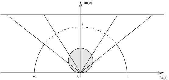
Figure 1: Eigenvalues corresponding to Klaus-Shaw potentials can not live in the shaded region near the origin. The symmetries of the problem then give a compact region where eigenvalues of (10) can live off the unit circle.

Finally, it follows by applying the transformation $z\to\frac{1}{z}$, there is an upper bound on ${\rm Im}(z)$ for eigenvalues of (10) (see figure 1). ∎

Corollary 2.

If $u$ satisfies the hypothesis of Theorem 2, then there exists an $R>0$ such that $B(0,R)\cap\sigma_{p}=\emptyset$.

It follows from the argument principle that discrete eigenvalues can only emerge from the continuous spectrum at $z=\pm 1$. Hence, if $Q_{top}=0$, the only way to have a eigenvalue off the unit circle is to have two eigenvalues on the unit circle collide to form a double eigenvalue, then bifurcate off the unit circle in a symmetry pair. Note that by Lemma 3, if $z$ is a discrete eigenvalue of (10) whose eigenspace has a definite Krein signature, then the corresponding eigenspace is semisimple, and hence simple. Thus, such collisions can never happen for potentials satisfying the hypothesis of Theorem 1, and can only occur in the sector $S$ if the potential satisfies the hypothesis of Theorem 2. The next theorem gives an analytic proof of this result which shows the explicit dependence on the definiteness of the Krein signature.

Theorem 4.

If $u$ satisfies the hypothesis of Theorem 1, then all the corresponding eigenvalues are simple. Moreover, if $u$ satisfies the hypothesis of Theorem 2, then all eigenvalues in the region $\left\{z=r\exp(i\theta):0<\theta\leq\frac{\pi-u_{0}}{2}\right\}$ are simple.

Proof.

This proof follows that given for Klaus and Shaw’s analogous result for the Zhakarov-Shabat system (see [10]). We define the Wronskian of $\Psi$ and $\Phi$ to be $W(\Psi,\Phi)=\psi_{1}\phi_{2}-\psi_{2}\phi_{1}$ where $\Psi$ and $\Phi$ are the Jost solutions defined in (16) or (22), depending of course on the value of $Q_{top}$. We say $z$ is a double eigenvalue of (10) if $\dot{W}(\Psi,\Phi)(x,z)=0$ where $\dot{a}$ denotes differentiation of $a$ with respect to $z$. We now derive an expression for $\dot{W}(\Psi,\Phi)(x,z)$ using the eigenvalue problem (10).

If $\vec{v}$ is an $L^{2}$ eigenfunction corresponding to an eigenvalue $z$ of (10), then it must be a multiple of both $\Phi$ and $\Psi$, and hence there exists a non-zero constant $C$ such that $\Psi=C\Phi$. Then if $W(z):=W(\Psi,\Phi)(x,z)$, which is independent of $x$, we have

$$\dot{W}(z) = W(\dot{\Psi},\Phi)+W(\Psi,\dot{\Phi})$$

$$= C\;W(\dot{\Psi},\Psi)+\frac{1}{C}\;W(\Phi,\dot{\Phi}).$$

Now, the fundamental theorem of calculus implies

$$W(\dot{\Psi},\Psi)(x,z)-W(\Psi,\dot{\Psi})(-x,z)=\int_{-x}^{x}\left(\dot{\psi}_{1}\psi_{2}-\dot{\psi}_{2}\psi_{1}\right)_{t}dt.$$

Using $r=1$ in (10), a tedious calculation yields

$$\left(\dot{\psi}_{1}\psi_{2}-\dot{\psi}_{2}\psi_{1}\right)_{t}=\frac{1}{2z}\left(\sin\theta\sin\left(\frac{u}{2}\right)\left(\psi_{1}^{2}-\psi_{2}^{2}\right)-2i\cos\theta\cos\left(\frac{u}{2}\right)\psi_{1}\psi_{2}\right).$$

Since $\Psi$ and $\Phi$ decay exponentially in their respective directions, it follows that

$$\lim_{x\to\infty}W(\dot{\Psi},\Psi)(x,z) = 0\;\;\rm{and}$$

$$\lim_{x\to-\infty}W(\Phi,\dot{\Phi})(x,z) = 0.$$

Therefore, if $z$ is an eigenvalue of (10),

$$\dot{W}(z) = \lim_{x\to\infty}\left(C\;W(\dot{\Psi},\Psi)(-x,z)+\frac{1}{C}\;W(\Phi,\dot{\Phi})(x,z)\right)$$

$$= C\lim_{x\to\infty}W(\dot{\Psi},\Psi)(-x,z)$$

$$= -\frac{C}{2z}\left(\sin\theta\int_{\mathbb{R}}\sin\left(\frac{u}{2}\right)\left(\psi_{1}^{2}-\psi_{2}^{2}\right)dt-2i\cos\theta\int_{\mathbb{R}}\cos\left(\frac{u}{2}\right)\psi_{1}\psi_{2}dt\right).$$

Recall that if $r=1$ then $\psi_{1}$ can be chosen to be real and $\psi_{2}$ to be purely imaginary. Hence, $\dot{W}(z)$ is non-zero by Theorems 1 and 2. ∎

Thus, if $Q_{top}=\pm 1$, all the eigenvalues lie on the unit circle and are simple. For Klaus-Shaw potentials discussed in Theorem 2, Theorem 4 implies all the eigenvalues $z=r\exp(i\theta)$ with $0<\theta\leq\frac{\pi-u_{0}}{2}$ lie on the unit circle are simple. Notice the above theorems do not contain much information about eigenvalues in the sector $S$: this stems from the fact that we do not have a definite Krein signature estimate there. In order to obtain a more complete description of the discrete spectrum in S, we use the above results to derive a lower bound on the number of eigenvalues of (10). Then, we use a homotopy argument to prove the eigenvalues in $S$ must be simple and lie on the unit circle. This is one of the main results of the next section.

5 Counting Eigenvalues

We now turn to the problem of counting the number of discrete eigenvalues associated with (10) for a given a potential $u$. As mentioned in the introduction, Klaus and Shaw were able to derive an exact count of the number of discrete eigenvalues of (2) in terms of the $L^{1}$ norm of the potential $q$ (see [11]). In this section, we derive an analogous result for the eigenvalue problem (10): we show the number of discrete eigenvalues is determined by the $L^{1}$ norm of $\sin\left(\frac{u}{2}\right)$.

To motivate such a result, consider a monotone potential with $Q_{top}=1$ with compactly supported gradient. Let $M(z;u)$ be the transfer matrix across the support of the gradient, assumed for simplicity to be $[-d,d]$. Since eigenvalues in the positive quadrant must initially emerge with multiplicity one from $z=1$, Theorem 4 implies that an upper bound on the number of discrete eigenvalues of (10) can be obtained by counting how many times $z=1$ is an eigenvalue. Furthermore, explicitly solving (10) at $z=1$ yields

$$M(z=1;u)\left(\begin{array}[]{c}1\\ 0\\ \end{array}\right)=\left(\begin{array}[]{c}\cos\left(\frac{1}{2}\int_{-d}^{d}\sin\left(\frac{u}{2}\right)dx\right)\\ i\sin\left(\frac{1}{2}\int_{-d}^{d}\sin\left(\frac{u}{2}\right)dx\right)\\ \end{array}\right).$$ (33)

From (16), the eigenvalue condition becomes

$$M(z=1;u)\left(\begin{array}[]{c}1\\ 0\\ \end{array}\right)\propto\left(\begin{array}[]{c}1\\ 0\\ \end{array}\right)$$

and thus, by applying a homotopy argument in the width of the support of $u^{\prime}$, our monotonicity assumption implies the $L^{1}$ norm of $\sin\left(\frac{u}{2}\right)$ determines the number of discrete eigenvalues of (10), as promised. A similar argument for potentials with $Q_{top}=0$ holds: however, since Theorem 4 does not guarantee all eigenspaces are simple, this only gives an upper bound on the number of discrete eigenvalues. However, by employing another counting scheme, we derive a lower bound on the number of eigenvalues of (10) which happens to overlap with our upper bound at only one point.

Although all of our main results will be concerned with potentials of the type considered in Theorem 1 and 2, unless otherwise stated we assume nothing about the structure of the potential $u$ other than that it decays to zero at $\pm\infty$ sufficiently rapidly that $\left(1-\left|\cos\left(\frac{u}{2}\right)\right|\right),\;\sin\left(\frac{u}{2}\right)\in L^{1}(\mathbb{R})$, and (again for simplicity) $u\in C^{1}(\mathbb{R})$. We first consider the case of a compactly supported potential. After extending these results to potentials considered in Theorem 2, we finish this section by stating the analogous results for potentials with $Q_{top}=\pm 1$. Throughout this section we only concern ourselves with counting the number of eigenvalues in the first quadrant of the upper half plane.

5.1 $Q_{top}=0$: Compact Support Case

One of the main goals of this section is to obtain confinement of the discrete spectrum to the unit circle for any potential satisfying the hypothesis of Theorem 2. To this end, we employ two different counting schemes to determine the number of points in the discrete spectrum. First, we count the number of points on the unit circle corresponding to eigenvalues of (10). This will provide a lower bound on the total number of eigenvalues. Since we know discrete eigenvalues must emerge initially from the continuous spectrum, Theorems 3 and 4 imply we can obtain an upper bound on the number of discrete eigenvalues of (10) by counting them as they emerge from the point $z=1$. This is the essence of the second counting scheme. The goal is to show that for potentials satisfying the hypothesis of Theorem 2, these two bounds agree.

We assume throughout this section $u$ is non-negative and compactly supported in the interval $[-d,d]$. Let $\overline{M}(z;u)$ denote the transfer matrix across the support of $u$. Due to the structure of the Jost solutions defined in (22) and the form of (10) outside the support of $u$, the eigenvalue condition becomes $\phi_{1}(d)=0$. Indeed, similar considerations imply the left boundary conditions $\phi_{1}(-d)=1$ and $\phi_{2}(-d)=0$, and thus $z$ is an eigenvalue of (10) if and only if

$$\overline{M}(z;u)\left(\begin{array}[]{cc}1\\ 0\end{array}\right)\propto\left(\begin{array}[]{cc}0\\ 1\end{array}\right).$$ (34)

First, we count the number of points on the unit circle in the open positive quadrant which correspond to discrete eigenvalues of (10). Let $z=\exp(i\theta)$ for $\theta\in[0,\frac{\pi}{2}]$ and employ a Prüfer transformation in (10):

$$\left(\begin{array}[]{c}\phi_{1}\\ i\phi_{2}\\ \end{array}\right)=\left(\begin{array}[]{c}\rho\cos\eta\\ \rho\sin\eta\\ \end{array}\right).$$ (35)

Then for a fixed $\theta$, $\rho(x;\theta)$, and $\eta(x;\theta)$ satisfy the coupled system of differential equations

$$-2\eta^{\prime} = \cos\theta\sin\left(\frac{u}{2}\right)+\sin\theta\cos\left(\frac{u}{2}\right)\sin(2\eta)$$ (36)

$$2\rho^{\prime} = \sin\theta\cos\left(\frac{u}{2}\right)\rho\cos(2\eta)$$

subject to the boundary conditions

$$\eta(-d;\theta)=0\quad{\rm and}\quad\rho(-d,\theta)=1.$$

As usual, the eigenvalue condition can be translated to a condition on the Prüfer angle variable. Indeed, $\exp(i\theta)$ is an eigenvalue of (10) if and only if $\eta(d;\theta)=\frac{2k-1}{2}\pi$ for some $k\in\mathbb{Z}$ (since then the boundary condition $\phi_{1}(d)=0$ is satisfied).

If $\theta=0$, then (36) reduces to $-2\eta^{\prime}=\sin\left(\frac{u}{2}\right)$ and hence

$$-2\int_{-d}^{d}\eta^{\prime}dx=-2\eta(d;0)=\int_{-d}^{d}\sin\left(\frac{u}{2}\right)dx.$$

Defining $I:=\int_{-d}^{d}\sin\left(\frac{u}{2}\right)dx$, we have $\eta(d;0)=-\frac{1}{2}I$. Similarly, letting $\theta=\frac{\pi}{2}$ in (36) gives

$$-2\eta^{\prime}=\cos\left(\frac{u}{2}\right)\sin\left(2\eta\right).$$

Since the right hand side is clearly Lipschitz, the initial condition $\eta\left(-d;\frac{\pi}{2}\right)=0$ implies $\eta\left(d;\frac{\pi}{2}\right)=0$. Thus, we immediately get the following lower bound on the total number of eigenvalues of (10).

Theorem 5.

Let $u\in C^{1}(\mathbb{R})$ have compact support, and let $N$ be the largest non-negative integer such that $|I|>(2N-1)\pi$. Then there exists at least $N$ eigenvalues of (10) on the unit circle in the open positive quadrant. In particular, if $|I|>\pi$, then there exists at least one eigenvalue on the unit circle.

Proof.

It follows from the continuity of $\eta(d;\cdot)$ that there exists $0<\theta_{1}<\theta_{2}<...<\theta_{N}<\frac{\pi}{2}$ such that

$$|\eta(d;\theta_{k})|=(2(N-k)+1)\frac{\pi}{2}$$

for each $k=1,2,...,N$. ∎

In the case where $u$ satisfies the hypothesis of Theorem 2 with $\frac{\pi}{2}<u_{0}<\pi$, the above counting scheme offers no improvement. However, if we know all the discrete eigenvalues of (10) lie on the unit circle and are simple, Theorem 5 produces an exact count.

Lemma 5.

Suppose $u$ is a compactly supported potential satisfying the hypothesis of Theorem 2 with $\|u\|_{L^{\infty}(\mathbb{R})}\leq\frac{\pi}{2}$. Then if N is defined as above, then there exists exactly N eigenvalues of (10), all of which live on the unit circle and are simple.

Proof.

We will prove monotonicity of $\eta(d;\theta)$ with respect to $\theta$ at an eigenvalue. By definition, $\tan\eta=i\frac{\phi_{2}}{\phi_{1}}$. Differentiating this with respect to $\theta$ and using the relation $\cos\eta=\frac{\phi_{1}}{\rho}$ we get

$$\dot{\eta}(d;\theta)=-\frac{i}{|\Phi|^{2}}\left(\dot{\phi}_{1}(d)\phi_{2}(d)-\phi_{1}(d)\dot{\phi_{2}}(d)\right),$$

where $\dot{f}:=\frac{df}{d\theta}$. Using (10) to integrate the above equation, noting that $\dot{\phi_{1}}(-d)=\dot{\phi_{2}}(-d)=0$ from the boundary conditions, we have

$$\dot{\eta}(d;\theta)=\frac{1}{2|\Phi(d)|^{2}}\left(\sin\theta\int_{-d}^{d}\sin\left(\frac{u}{2}\right)(\phi_{1}^{2}-\phi_{2}^{2})dx-2i\cos\theta\int_{-d}^{d}\cos\left(\frac{u}{2}\right)\phi_{1}\phi_{2}dx\right)$$

which is always positive at an eigenvalue. This rules out multiple crossings of $\eta(d;\theta)=\frac{2k-1}{2}\pi$ and hence there are exactly N eigenvalues of (10), all of which live on the unit circle and are simple by Theorems 2 and 4.∎

The failure of the above counting scheme for a general potential satisfying the hypothesis of Theorem 2 arises from the fact that it does not respect the multiplicity of the eigenvalues. However, it does produce the exact number of points on $S^{1}\cap\{w=a+ib:a,b\in\mathbb{R^{+}}\},$ which correspond to an eigenvalue of (10). We now obtain an upper bound on the number of eigenvalues by counting them as they emerge from the continuous spectrum.

To this end, we employ a homotopy argument in the height of a potential $u$ satisfying the hypothesis of Theorem 2 and the condition $\frac{\pi}{2}<\|u\|_{L^{\infty}}<\pi$. For each such $u$, define a one parameter family of potentials $u_{a}(x):=au(x)$ for $a\in[0,1]$. For small enough values of $a$, Theorems 2 and 4 imply the discrete eigenvalues lie on the unit circle and are simple. Defining $I(a):=\int_{-d}^{d}\sin\left(\frac{u_{a}}{2}\right)dy$, (34) implies that an upper bound on the total number of eigenvalues of (10) is given by the total number of zeroes of the function

$$F(a):=\cos\left(\frac{1}{2}I(a)\right)$$

on $[0,1)$. Since $I(0)=0$ and $I$ is an increasing function of $a$, we immediately see that if $N$ is the largest non-negative integer such that $I(1)>(2N-1)\pi$, then there exists a total of at most $N$ discrete eigenvalues of (10) in the positive quadrant. Thus, we see the $N$ given by Theorem 5 is also an upper-bound on the total number of eigenvalues of (10) in the positive quadrant. This proves the following improvement of Theorem 2.

Theorem 6.

Let $u$ be a compactly supported potential satisfying the hypothesis of Theorem 2. Let $N$ be the largest non-negative integer such that $\int_{-d}^{d}\sin\left(\frac{u}{2}\right)dx>(2N-1)\pi$. Then there exists exactly $N$ discrete eigenvalues of (10) in the open positive quadrant, all of which lie on the unit circle and are simple.

Proof.

The above homotopy argument proves the discrete spectrum lies on the unit circle. Recalling that the count obtained from Theorem 5 does not respect the multiplicities of the eigenvalues completes the proof. ∎

Noting that when $u\equiv 0$ the discrete spectrum is empty, we see that if $u$ satisfies the hypothesis of Theorem 2 then $\pi$ is the threshold $L^{1}$ norm for $\sin\left(\frac{u}{2}\right)$ for the existence of discrete eigenvalues for (10). We now prove this threshold persists for a more general class of potentials.

Theorem 7.

Let $u\in C^{1}(\mathbb{R})$ have compact support, be of fixed sign, and satisfy $\|u\|_{L^{\infty}}\leq\pi$. If

$$\left|\int_{-d}^{d}\sin\left(\frac{u}{2}\right)dx\right|\leq\pi,$$

then there do not exist any eigenvalues of (10) on the unit circle.

To prove the theorem, we will use the following Gronwall type result[11].

Lemma 6 (Comparison Theorem).

Let the function $f(t,y)$ satisfy a local Lipschitz condition in $y$ and define the operator $P$ by $P(g)=g^{\prime}-f(t,g)$. Let $g_{1}$ and $g_{2}$ be absolutely continuous functions on $[t_{1},t_{2}]$ such that $g_{1}(t_{1})\leq g_{2}(t_{1})$ and $P(g_{1})\leq P(g_{2})$ almost everywhere on $[t_{1},t_{2}]$. Then either $g_{1}(t)<g_{2}(t)$ everywhere in $[t_{1},t_{2}]$, or there exists a point $c\in(t_{1},t_{2})$ such that $g_{1}(t)=g_{2}(t)$ in $[t_{1},c]$ and $g_{1}(t)<g_{2}(t)$ in $(c,t_{2}]$.

We are now prepared to prove the theorem.

Proof of Theorem.

With out loss of generality, assume $u\geq 0$ on $\mathbb{R}$. Note that if $u\equiv 0$, then the theorem is trivially true. Suppose now that supp$(u)=[-d,d]$ for some $d>0$. The goal is to show $|\eta(d;\theta)|<\frac{\pi}{2}$ for all $0<\theta<\frac{\pi}{2}$. We use the comparison theorem on $[a,b]$ with

$$P(g):=g^{\prime}+\frac{1}{2}\cos\theta\sin\left(\frac{u}{2}\right)+\frac{1}{2}\sin\theta\cos\left(\frac{u}{2}\right)\sin(2g).$$

Since $\eta(-d;\theta)=0$ and $P(0)=\frac{1}{2}\cos\theta\sin\left(\frac{u}{2}\right)\geq P(\eta)=0$, we see

$$\eta(x;\theta)\leq 0\quad{\rm for}\;\;-d\leq x\leq d.$$

Now, if we let $g(x;\theta)=-\frac{1}{2}\cos\theta\int_{-d}^{x}\sin\left(\frac{u}{2}\right)dt$, then $g(-d;\theta)=0$ and

$$P(g)=\frac{1}{2}\sin\theta\cos\left(\frac{u}{2}\right)\sin\left(-\cos\theta\int_{-d}^{x}\sin\left(\frac{u}{2}\right)dt\right).$$

Since $\sin\left(\frac{u}{2}\right)\in L^{1}(\mathbb{R})$, $P(g)\leq 0=P(\eta)$ and hence we have

$$\left|\eta(x;\theta)\right|\leq\frac{1}{2}\cos\theta\int_{-d}^{x}\sin\left(\frac{u}{2}\right)dt\quad{\rm for}\;\;-d\leq x\leq d.$$

Now, unless $u\equiv 0$, strict inequality must hold at $x=d$. For if we had equality, then by the comparison theorem

$$\eta(x;\theta)=-\frac{1}{2}\cos\theta\int_{-d}^{x}\sin\left(\frac{u}{2}\right)dt\quad{\rm for}\;\;-d\leq x\leq d.$$

and hence from (36) we have $\sin(2\eta)\equiv 0$, i.e. $\eta(x;\theta)\equiv 0$. But this implies $\sin\left(\frac{u}{2}\right)\equiv 0$ and hence we must have $u\equiv 0$. Thus,

$$|\eta(d;\theta)|<\frac{1}{2}\cos\theta\int_{-d}^{d}\sin\left(\frac{u}{2}\right)dx.$$

Hence, there can be no eigenvalues if $\int_{-d}^{d}\sin\left(\frac{u}{2}\right)dx\leq\pi$, as claimed. ∎

5.2 $Q_{top}=0$: General Case

We now extend the above results for the case where the potential $u$ is not compactly supported. We employ the Prüfer transformation (35), where the angular variable $\eta$ is required to satisfy the boundary condition

$$\lim_{x\to-\infty}\eta(x;\theta)=0.$$ (37)

Since the eigenvalue condition becomes $\lim_{x\to\infty}\phi_{1}(x)=0$, we must analyze the behavior of the function $L_{\eta}(\theta):=\lim_{x\to\infty}\eta(x;\theta)$ for $\theta\in\left[0,\frac{\pi}{2}\right)$. Notice that $z=e^{i\theta}$ is an eigenvalue if $L_{\eta}(\theta)=(2N-1)\frac{\pi}{2}$ for some integer $N$.

Setting $\theta=0$ in (10), we see immediately $L_{\eta}(0)=\int_{\mathbb{R}}\sin\left(\frac{u}{2}\right)dx$ as before. When we set $\theta=\frac{\pi}{2}$, it is not clear if the zero solution is the unique solution to the resulting problem (due to the boundary condition). This uncertainty is handled in the following lemma.

Lemma 7.

If $u$ satisfies the hypothesis of Theorem 2, then the unique solution to the differential equation

$$-2\eta^{\prime}=\cos\left(\frac{u}{2}\right)\sin\left(2\eta\right)$$

subject to (37) is $\eta(x)\equiv 0$.

Proof.

The corresponding integral equation for $\eta$ is

$$-2\eta(x)=\int_{-\infty}^{x}e^{-\int_{y}^{x}\cos\frac{u}{2}dw}\cos\left(\frac{u}{2}\right)\left(\sin\left(2\eta\right)-2\eta\right)dy.$$

Let $M(x):=\sup_{-\infty<s<x}\left|\eta(x)\right|$. Using the inequality $|\sin(y)-y|<\frac{1}{6}|y|^{3}$ for all $y\in\mathbb{R}$, along with the estimate

$$\int_{-\infty}^{x}e^{-\int_{y}^{x}\cos\frac{u}{2}dw}dy\leq\sec\left(\frac{u_{0}}{2}\right),$$

we see $M(x)$ satisfies

$$M(x)\leq C\left(M(x)\right)^{3}$$

for all $x\in\mathbb{R}$, where $C:=\frac{1}{12}\sec\left(\frac{u_{0}}{2}\right)$. Since $\eta$ is a continuous function of $x$, this implies that either $M(x)=0$ for all $x\in\mathbb{R}$, or else $M(x)\geq C^{-1/2}$ for all $x\in\mathbb{R}$. Since $\lim_{x\to-\infty}M(x)=0$, we must have $M(x)\equiv 0$. ∎

It is now straight forward to verify that Theorem 5 and Theorem 6 hold for any potential $u$ satisfying the hypothesis of Theorem 2. In particular, we have now proven our main result for the locations of the eigenvalues of (10).

Theorem 8.

Suppose $u\in C^{1}(\mathbb{R})$ is a potential such that $\sin\left(\frac{u}{2}\right)\in L^{1}(\mathbb{R})$ is of fixed sign, has exactly one critical point, and $\left(1-\left|\cos\left(\frac{u}{2}\right)\right|\right)\in L^{1}(\mathbb{R})$. Then all the eigenvalues of (10) lie on the unit circle and are simple.

Remark 6.

Remark 5 holds for any potential satisfying the hypothesis of Theorem 2.

5.3 $Q_{top}=\pm 1$: General Case

We now prove the analogues of the above results for potentials $u$ satisfying the hypothesis of Theorem 1. For definiteness, assume $Q_{top}=1$. In this case, we consider (10) with boundary conditions

$$\lim_{x\to-\infty}\left(\begin{array}[]{cc}\phi_{1}(x)\\ \phi_{2}(x)\\ \end{array}\right)=\left(\begin{array}[]{cc}1\\ 0\\ \end{array}\right)$$

and note that, due to the structure of the Jost solutions, the eigenvalue condition becomes $\lim_{x\to\infty}\phi_{2}(x)=0$. Using the Prüfer transformation (35), we see that $\eta(x;\theta)$ must satisfy (36) with the boundary condition (37), where the eigenvalue conditions becomes $\lim_{x\to\infty}\eta(x;\theta)=k\pi$ for some $k\in\mathbb{Z}$. As above, we have that

$$I:=\int_{-\infty}^{\infty}\sin\left(\frac{u}{2}\right)dx=-2L_{\eta}(0),$$

and Lemma 7 implies $L_{\eta}\left(\frac{\pi}{2}\right)=0$ Thus, we get the following result.

Theorem 9.

Let $u$ be a real potential satisfying Theorem 1. Let $N$ be the largest integer such that $I>2N\pi$. Then there exists exactly $2N+1$ eigenvalues of (10) in the $UHP$, all of which live the unit circle and are simple.

Remark 7.

Note that if $u$ is not monotone, replacing $I$ with $|I|$ gives a lower bound on the number of eigenvalues of (10).

Proof.

Simply notice that if $I>2N\pi$, then $|L_{\eta}(0)|>N\pi$. Since $L_{\eta}\left(\frac{\pi}{2}\right)=0$, we know there exists $\theta_{1},\;\theta_{2}\;,\;...\;,\;\theta_{N}\in\left(0,\frac{\pi}{2}\right)$ such that $z_{k}=e^{i\theta_{k}}$ is an eigenvalue of (10) for each $k=1,2,...,N$. By Theorems 1 and 4, and the proof of Lemma 5, we see the set $\{z_{k}\}_{k=1}^{N}$ consists of all the eigenvalues of (10) in the open positive quadrant. The theorem follows by recalling that $i$ is always an eigenvalue of (10) for kink-like data. ∎

Remark 8.

Note that by letting $x\to-x$, Theorem 9 holds with $I$ replaced with $-I$ when $Q_{top}=-1$.

6 Conclusions

In this paper we have proven a Klaus-Shaw type theorem for the Sine-Gordon scattering problem for kink-like potentials with topological charge $\pm 1$ (under the assumption of monotonicity) and for breather-like potentials under the assumption that the potential $u$ has a single maximum of height less than $\pi$. Note that this implies that $\sin(u/2)$ has a single maximum. The main analytical difficulty in dealing with the case where the height of the maximum is greater than $\pi$ is that we are no longer able to show that the eigenvalues emerge from the essential spectrum at $z=\pm 1$, so apriori eigenvalues can emerge from anywhere along the real axis with (potentially) arbitrary multiplicity. Using the techniques of this paper it is still straightforward to establish a lower bound (though not an upper bound) for the number of eigenvalues on the unit circle, but we have little or no information about the number of eigenvalues off of the unit circle.

Tentative numerical experiments have indicated that the first result is probably tight: monotone kinks of higher topological charge and non-monotone kinks of topological charge $\pm 1$ frequently have point eigenvalues which do not lie on the unit circle. Similar experiments on breather-like potentials suggests that this result may be improved. In particular for breather-like potentials with a single maximum we have not observed point spectrum off of the unit circle until the height of the maximum reaches $2\pi$. Geometrically there is some further evidence to support this: the monodromy matrix at $z=1$ has the property that the winding number is strictly increasing for Klaus-Shaw potentials of height less than $2\pi$. We are currently investigating whether an improvement of the theorem along these lines is possible.

It is interesting to note that there is no analog of these results in the periodic case, It is easy to compute that the Floquet discriminant of the problem always lies in the interval $[-2,+2]$ when $\lambda$ lies on the real axis. If the Floquet discriminant has a critical point on the interior $(-2,2)$ then by a simple analyticity argument the problem must have spectrum lying off of the real axis. Thus the only case in which the eigenvalue problem has spectrum confined to the union of the real axis and the unit circle is when all of the critical points of the Floquet discriminant on the real axis are double points. In this case the potential is necessarily a finite gap solution, and can be constructed by algebro-geometric methods.[1].

7 Appendix

In this section, we mention one of the more technical but standard results which are needed in making the above arguments rigorous. Namely, we prove that eigenfunctions of (10) are exponentially bounded as $x\to\infty$.

As mentioned in the introduction, for potentials $u$ satisfying $\lim_{x\to-\infty}u(x)=0$, $Q_{top}=1$, and, without loss of generality, $u(0)=\pi$, we define the “Jost” solutions of (10) by the asymptotic properties (16) and (22) for ${\rm Im}(z)>0$. Note that these solutions differ from the standard Jost solutions by a normalization at $\pm\infty$. From scattering theory, we know that up to constant multiples $\Psi$ and $\Phi$ are the unique solutions of (10) which are square integrable on $(-\infty,0]$ and $[0,\infty)$, respectively. It follows that if $\vec{v}$ is any eigenfunction of (10) corrresponding to an eigenvalue $z$, then $v$ must be a multiple of both $\Phi(x,z)$ and $\Psi(x,z)$.

To show exponential boundedness of the Jost solutions, we begin by factoring off the asymptotic behavior at $\pm\infty$. To this end, fix $z\in UHP$ and define $\widetilde{\Psi}(x):=\Omega(x)\Psi(x,z)$ and $\widetilde{\Phi}(x):=\Omega(x)\Phi(x,z)$ where

$$\Omega(x)=\exp\left(-\frac{1}{4}\left(z-\frac{1}{z}\right)\int_{x}^{0}\cos\left(\frac{u}{2}\right)dy\tau_{1}\right).$$

It follows that $\tilde{\Psi}$ and $\tilde{\Phi}$ are the unique solutions of the following system of integral equations:

$$\widetilde{\Psi}(x) = \left(\begin{array}[]{c}1\\ 0\\ \end{array}\right)+\frac{1}{4}\left(z+\frac{1}{z}\right)\int_{-\infty}^{x}\sin\left(\frac{u(y)}{2}\right)\Omega(y)^{-1}\tau_{2}\Omega(y)\widetilde{\Psi}(y)dy$$

$$\widetilde{\Phi}(x) = \left(\begin{array}[]{c}1\\ 0\\ \end{array}\right)+\frac{1}{4}\left(z+\frac{1}{z}\right)\int_{x}^{\infty}\sin\left(\frac{u(y)}{2}\right)\Omega(y)^{-1}\tau_{2}\Omega(y)\widetilde{\Phi}(y)dy.$$

The first of these is used to obtain bounds as $x\to-\infty$, while the second can be used to obtain similar bounds as $x\to\infty$. By standard arguments involving the contraction mapping principle, one can show that $\widetilde{\psi}_{1}\in L^{\infty}\left(-\infty,0\right)$, i.e.

$$\left|\psi_{1}(x,z)\right|\leq C\exp\left(-\frac{\beta}{4}\int_{x}^{0}\cos\left(\frac{u}{2}\right)dy\right)$$

for some $C>0$, where $\beta:={\rm Im}\left(z-\frac{1}{z}\right)$. Substituting this into the above integral equations, and noting that $\sin\left(\frac{u}{2}\right)$ is increasing on $(-\infty,0)$, yields

$$\frac{\left|\psi_{2}(x,z)\right|}{\left|z+\frac{1}{z}\right|}\leq C\sin\left(\frac{u}{2}\right)\exp\left(\frac{\beta}{4}\int_{x}^{0}\cos\left(\frac{u}{2}\right)dy\right)\int_{-\infty}^{x}\exp\left(-\frac{3\beta}{4}\int_{y}^{0}\cos\left(\frac{u}{2}\right)dy\right)$$

for $x<0$. In particular, this shows that if $\Psi$ is an eigenvector of (10), then $\csc\left(\frac{u}{2}\right)\psi_{2}\in L^{1}(-\infty,0)$ for any potential $u$ satisfying the hypothesis of Theorem 1. Similar results hold for $\phi_{1}$ and $\phi_{2}$ as $x\to\infty$. By letting $x\to-x$ above, it follows that eigenfunctions of (10) must be bounded and decay exponentially as $|x|\to\infty$ in the case $Q_{top}=\pm 1$. These results are vital in showing convergence of integrals when we study potentials with $Q_{top}=\pm 1$, as well as proving certain boundary terms arising from integration by parts vanish.

Similar arguments imply analogous results when $u$ satisfies the hypothesis of Theorem 2.

References

• [1] E.D. Beolokolos, A.I. Bobenko, V.Z. Enol’skii, A.R. IΒ ts, and V.B Matveev. Algebro-geometric approach to nonlinear integrable equations. Springer-Verlag, Berlin, 1994.
• [2] AlanΒ R. Bishop, Randy Flesch, M.Β Gregory Forest, DavidΒ W. McLaughlin, and EdwardΒ A. Overman, II. Correlations between chaos in a perturbed sine-Gordon equation and a truncated model system. SIAM J. Math. Anal., 21(6):1511–1536, 1990.
• [3] Harold Blas and HectorΒ L. Carrion. Solitons, kinks and extended hadron model based on the generalized sine-Gordon theory. J. High Energy Phys., 1:027, 27 pp. (electronic), 2007.
• [4] Robert Buckingham and PeterΒ D. Miller. Exact solutions of semiclassical non-characteristic cauchy problems for the sine-gordon equation. arXiv:nlin.si, 07053159:49 (electronic), 2007.
• [5] S.Β Cuenda, A.Β SΓ‘nchez, and N.Β Quintero. Does the dynamics of sine-gordon solitons predict active regions of dna? arXiv:q-bio.GN, 0606028:1–17, 2006.
• [6] L.Β D. Faddeev and L.Β A. Takhtajan. Hamiltonian methods in the theory of solitons. Springer Series in Soviet Mathematics. Springer-Verlag, Berlin, 1987. Translated from the Russian by A. G. Reyman [A. G. ReΔ­man].
• [7] J.Β D. Gibbon, I.Β N. James, and I.Β M. Moroz. An example of soliton behaviour in a rotating baroclinic fluid. Proc. Roy. Soc. London Ser. A, 367(1729):219–237, 1979.
• [8] RoyΒ H. Goodman and Richard Haberman. Interaction of sine-Gordon kinks with defects: the two-bounce resonance. Phys. D, 195(3-4):303–323, 2004.
• [9] D.J. Kaup. Method for solving the sine-gordon equation in laboratory coordinates. Studies in Appl. Math., 54(2):165–179, 1975.
• [10] M.Β Klaus and J.Β K. Shaw. Purely imaginary eigenvalues of Zakharov-Shabat systems. Phys. Rev. E (3), 65(3):036607, 5, 2002.
• [11] M.Β Klaus and J.Β K. Shaw. On the eigenvalues of Zakharov-Shabat systems. SIAM J. Math. Anal., 34(4):759–773, 2003.
• [12] GeorgeΒ L. Lamb, Jr. Elements of soliton theory. John Wiley & Sons Inc., New York, 1980. Pure and Applied Mathematics, A Wiley-Interscience Publication.
• [13] E.Β Lennholm and M.Β HΓΆrnquist. Revisiting Salerno’s sine-Gordon model of DNA: active regions and robustness. Physica D Nonlinear Phenomena, 177:233–241, March 2003.
• [14] M.Β Salerno. Discrete model for dna promoter dynamics. Phys. Rev. A, 44(8):5292–5297, 1991.
• [15] AlwynΒ C. Scott. Magnetic flux annihilation in a large Josephson junction. In Stochastic behavior in classical and quantum Hamiltonian systems (Volta Memorial Conf., Como, 1977), volumeΒ 93 of Lecture Notes in Phys., pages 167–200. Springer, Berlin, 1979.
• [16] Eli Shlizerman and Vered Rom-Kedar. Hierarchy of bifurcations in the truncated and forced nonlinear SchrΓΆdinger model. Chaos, 15(1):013107, 22, 2005.
• [17] Chuu-Lian Terng and Karen Uhlenbeck. Geometry of solitons. Notices Amer. Math. Soc., 47(1):17–25, 2000.
• [18] V.A. Yakubovich and V.M. Starzhinskii. Linear Differential Equations with Periodic Coefficients I,II. Wiley, 1975.
• [19] S.Β Yamosa. Soliton excitations in deoxyribonucleic acid (dna). Phys. Rev. A, 27(4):2120–2125, 1983.
• [20] V.Β E. Zaharov, L.Β A. TahtadΕΎjan, and L.Β D. Faddeev. A complete description of the solutions of the β€œsine-Gordon” equation. Dokl. Akad. Nauk SSSR, 219:1334–1337, 1974.