Otiy: Locators Tracking Nodes

Abstract

We propose Otiy, a node-centric location service that limits the impact of location updates generate by mobile nodes in IEEE 802.11-based wireless mesh networks. Existing location services use node identifiers to determine the locator (aka anchor) that is responsible for keeping track of a node’s location. Such a strategy can be inefficient because: (i) identifiers give no clue on the node’s mobility and (ii) locators can be far from the source/destination shortest path, which increases both location delays and bandwidth consumption. To solve these issues, Otiy introduces a new strategy that identifies nodes to play the role of locators based on the likelihood of a destination to be close to these nodes – i.e., locators are identified depending on the mobility pattern of nodes. Otiy relies on the cyclic mobility patterns of nodes and creates a slotted agenda composed of a set of predicted locations, defined according to the past and present patterns of mobility. Correspondent nodes fetch this agenda only once and use it as a reference for identifying which locators are responsible for the node at different points in time. Over a period of about one year, the weekly proportion of nodes having at least 50% of exact location predictions is in average about 75%. This proportion increases by 10% when nodes also consider their closeness to the locator from only what they know about the network.

1 Introduction

Promoting node mobility in self-organizing wireless networks implies setting up an efficient location management scheme. Indeed, the degree of node mobility impacts the amount of location updates disseminated throughout the network; this problem becomes even more critical in dense areas, where the profusion of signaling messages induces serious contentions and penalizes the overall performance of applications.

There are different techniques to implement location services. In flooding-based approaches, no proactive decision is made; when a source wants to communicate with a destination, it floods the entire network with a lookup message. Although simple, such an approach is very resource consuming and thus inappropriate for wireless networks. In order to solve this problem, some solutions propose to use location anchors – when a source wants to communicate with a destination, it must first ask the anchor about the current location of the node. Anchor-based architectures can be implemented in a centralized or distributed manner [2, 7, 13, 15]. Nevertheless, these solutions share a common pitfall: they have no control on the location of the anchor. This means that a source may have to send a lookup message to a far-away anchor for a destination that is possibly nearby. The consequences are twofold: (i) lookup phase may experience large delays and (ii) lookup messages may travel long distances, reducing the overall capacity of the network. The consequences are the same for the destination node which also have to update its current location to a possibly far-away responsible (or assigned) anchor.

To address the abovementioned problems, we propose Otiy, a two-tiered location service that relies on the fact that most nodes present cyclic mobility patterns. Indeed, many works have shown that, in many situations, nodes do show mobility characteristics that can be quite well predicted based on the node’s mobility history [1, 5, 8, 16, 17].

Otiy benefits from mobility prediction by decoupling the location service into two tiers as follows:

1. Global service. This service determines the anchor of a node, in a similar way to traditional solutions. The difference here is that anchors in Otiy do not store the current location of nodes; instead, it returns an agenda containing for each period of the day the location server (or locator, cf., next bullet) which is most probably the closest to the mobile node. This agenda is available for a reasonable amount of time and thus can be stored by the communicating nodes to prevent frequent access to the global service.

2. Local service. Locators are points in the infrastructure that effectively know at a given time where mobile nodes are. They respond to lookup requests and inform about the current position of mobile nodes. To determine which of its locators is currently in charge of storing its location, a mobile node refers to its agenda. As a locator is chosen by a mobile node because of its high probability of being close to it, location updates remain localized.

The idea behind this system is to use the global service from time to time and the local service most of the time – and thus reduce the overhead found in flat solutions. More specifically, an agenda contains a list of pairs ${\tt(Time\_slot,Locator)}$, where for the time period ${\tt Time\_slot}$ the location information of the mobile node will be managed by ${\tt Locator}$. This agenda remains valid for a certain period, after which it must be renewed at the corresponding $anchor$. A source willing to communicate with a destination first fetches the agenda of the destination at its corresponding anchor. Then, during the validity period of the agenda – which can last for weeks depending on the prediction accuracy – the source only contacts locators to obtain the exact location of the destination. The generation of a pertinent agenda to identify the best locator (closest to the mobile node) for each time slot is thus at the heart of Otiy. We argue that mobile nodes don’t necessarily have a positioning system and should therefore determine their mobility pattern based only on topological information, meaning the logs of attachment to the access points.

Although the basic concepts of Otiy can be generalized to different types of self-organizing wireless networks, in this paper we focus on the context of wireless mesh networks (WMN) composed of IEEE 802.11 access points (mesh routers). In this case, mobility is defined as a sequence of access points a node associates to along time. We will see later in this paper that defining exact mobility patterns in a wireless mesh network is a complex task. For instance, misinterpretations of mobility may happen mainly due to ping-pong effects, which are oscillations of associations/disassociations to nearby mesh routers due to changes in medium conditions. In order to address this problem, we introduce a self-organizing scheme that groups nearby mesh routers into clusters from each node standpoint. This clustering scheme masks ping-pong effects and allows reducing the space of possible locations.

We evaluate Otiy under a large population of nodes using real traces of mobility in a campus scenario [9]. We find that nodes, although heterogeneous in nature, do show cyclic behaviors according to their own rules. The analysis covers periods ranging from one month to more than one year and presents results in function of the number of active nodes and the different periods animating the campus (e.g., holidays, school periods, weekends). From the observations, the weekly proportion of nodes having at least 50% of exact location predictions is in average about 75%. This proportion increase by 10% if nodes also consider known properties on the deployment area (e.g., buildings, offices, paths).

In Section 2, we present the rationale for a node-centric approach and introduce Otiy’s architecture. In Section 3.2, we present our algorithm to readapt the association logs and to elect the appropriate locators. In Section 3.3, we analyze the cyclicity and the persistence of the nodes’ behaviors upon which is based Otiy. In Section 4, we evaluate the agendas accuracy according to the wireless data traces from the Dartmouth campus. We delay our discussion of related work until Section 5 in order to have enough context to make the necessary connections. We finally present some conclusion in Section 6.

2 Otiy’s design

Otiy introduces a different approach for distributed location services in wireless mesh networks. In this section we first motivate our proposal and then present Otiy’s architecture and operation. For lack of space, many details are omitted.

2.1 Rationale

We consider wireless mesh networks with following characteristics: (i) resources are scarce (wireless medium), (ii) the backbone is static, (iii) nodes are mobile, and (iv) the backbone can be highly dense (e.g., for over-provisioning) in localized hotspot areas. In such a context, which is expected to happen in many situations, the networking architecture becomes fully dependent on an efficient location service. An “efficient” location service should have at least the following characteristics:

1. Location updates do not interfere much with the network operations.

2. Location signaling messages have low latency.

3. Location information is accurate.

This paper provides a response to these three requirements. We base our reasoning on the possibility of having persistent location information (i.e., with long validity duration) – location updates to the anchor (called location dissemination in the rest of the paper) become then more spaced in time, which reduces the amount of propagated signaling messages. This is the response to requirement #1 above.

To provide persistent location information, we take as a premise that different nodes have different levels of mobility. Many studies in the literature have shown that there is a large part of predictability in how nodes move at an AP [8, 12, 4] granularity. Location services that are based on these studies use prediction to precisely identify the APs to which nodes will be associated with. Nevertheless, the presence of the ping-pong effect and the development of cognitive radio can have major impact on the efficiency of these approaches.

In Otiy, we take a different approach. Instead of trying to obtain the exact location of a node, we use the node’s past and present mobility pattern to distribute locators throughout the network. With high probability (as shown in Section 3.3), locator nodes are placed close to the current location of the node and so, close to the shortest path between sources and destinations. This responds to both requirements #2 and #3.

2.2 The reasons for node-centric mobility

We have identified four aspects related to the mobility of nodes:

• Periods of activity. Depending on the device type and the necessity to being connected, nodes can show completely different periods of activity, ranging from diurnal activity to sporadic connections only on week-ends.

• Mobility coverage. We refer to “mobility coverage” as the number of different APs visited during a single session. We observe that some nodes are aware of the roaming capabilities offered by their underlying network and take advantage of them, while others remain static or have only a nomadic behavior.

• Home location characterization. It is not always possible to identify for each node a home location (an area where a node spends more than 50% of its association time [6]). This parameter gives an indication on the regularity of the associations of the nodes to a specific location.

• Number of visited areas. This parameter is an extended view of the mobility coverage; the number of visited areas accounts for all visits of a node for the entire observed period (multiple sessions). Mobile or not, the disparities between nodes on this point are deep. The interest of visiting different APs in the network has clear relationship with the social interest of visiting different areas in the environment.

Interests, constraints, and motivations behind the patterns of mobility are manifold and have different impact on the complexity of network management. Furthermore, each node has its own mobility pattern, which itself varies in time. For these reasons, we advocate that, for a location service to be efficient, it must manage mobility at a node scale.

Otiy goes a bit further and proposes that nodes self-profile their behaviors. Such a node-centric approach consists in making nodes themselves log their sequence of associations together with timestamps and SSIDs. We show in the following how Otiy makes use of such information.

2.3 Agenda of locators

The key element of our proposal is the agenda of locators. The image of the agenda is important and contributes to highlight the relationship we want to give between a precise location and the considered time.

We delay our discussion of cyclicity of mobility until Section 3.3 in order to avoid interrupting our reasoning. In this way, we ask the reader to just assume for the moment that nodes have cyclic mobility.

2.3.1 Description

We define the agenda for node $n$ as table $A_{n}$. It is composed of $N$ columns defining the days of cycle and $M$ rows that give the granularity of the estimation we give to the node’s mobility. W.l.g., in this paper we consider a cycle of one week and a granularity of one hour (i.e., $N=7$ and $M=24$). The values of $N$ and $M$ will be motivated in Section 3.3). We also assign a validity period for the agenda, which is a multiple of $N$ representing the number of full cycles the agenda will remain unchanged (no updates will be provided).

To each time slot $a_{ij}$ (with $0\leq i<N$ and $0\leq j<M$) of an equal duration $D=\lceil\frac{24}{M}\rceil$ hour(s), is assigned one locator node. The choice of this locator depends on the mobility of the node observed during the same time slot in the past and is typically a mesh router network address.

We store the history of mobility pattern of node $n$ in a set of tables $H^{k}_{n}$ (of same dimensions as $A_{n}$), where $k\geq 0$ indicates the “age” of the table. We define $H_{n}^{0}$ as the table containing the current mobility of the node, $H_{n}^{1}$ the mobility of the precedent week and so on until $k=k_{\max}$ ($k_{\max}$ typically varies between 2 and 4). In each time slot $h_{i,j}^{k}$, the node records the location of the area at which the node spent most of its time during slot $j$ for the day $i$, $k$ weeks before, according to the mobility log file. In this way, we define a notion of prevalence of a particular area for a given time slot. Furthermore, for each $h_{i,j}^{0}$ the node records the duration of association $d(h_{i,j}^{0})$ (where $0<d(h_{i,j}^{0})\leq D$) of the selected location.

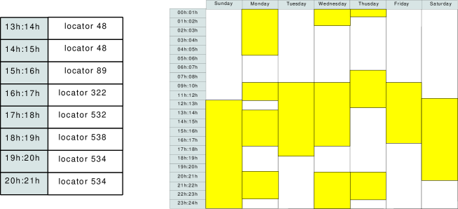
Figure 1: Example of a simplified agenda of associations.

At the end of each validity period, the node generates a new agenda based on its mobility history (as on Fig. 1). The resulting locator $a_{i,j}$ will depends on the oldness he have in the network, the necessary mobility history needed to provide an accurate location $k_{\max}$ (studied in Section 4), and the duration of association $d(h_{i,j}^{0})$.

We can now define the locator $a_{i,j}$ as:

$$a_{i,j}=\left\{\begin{array}[]{ll}h_{i,j}^{0}&\qquad\mathrm{if}\quad d(h_{i,j}^{0})=D\\ \text{maxoccur}(h_{i,j}^{0},...,h_{i,j}^{k_{max}})&\qquad\mathrm{otherwise,}\\ \end{array}\right.$$ (1)

In the case where $d(h_{i,j}^{0})=D$, we assume that the duration of association at this particular area has been greater than $D$. If in the node’s history it has always been the same area, then giving a higher weight to the latest observation does not improves the quality of the estimation. If it is a different area, we conclude that it indicates a deep change in the behavior of the node and then we select this locator for the agenda.

If $d(h_{i,j}^{0})<D$, we choose the locator which has the maximum number of occurrences in the mobility history for the same time slot (if equal, we choose the most recent locator). In this case, we can not judge on the persistence that $h_{i,j}^{0}$ will have in the future; in this way, we give more weight to the node’s habits for this time slot.

Scheme 1

To avoid holes in the agenda, we extend the locator of the preceding non empty slots to cover an empty time slot.

2.3.2 Bootstrap

For the first association in the network, the node $n$ generates an agenda $A_{n}$ where all $a_{i,j}$ are set to the location of the first visited mesh router. This agenda has a validity period until the end of the cycle (in our case the end of the week). At the end of this period, the new generated agenda will have logically the values given by $H_{n}^{0}$. After a longer period, the choice of the locators become more accurate because the node disposes of a larger history.

Scheme 2

The bootstrap procedure is executed for the first association in the network and also after long periods of inactivity. In this latter case, we observe that the behaviors of the nodes often become completely different (e.g., change of home location and different mobility pattern). The minimal duration of inactivity before a restart of the bootstrap is discussed in Section 4.

2.4 Location updates

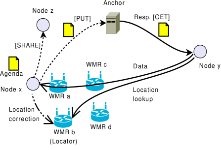
Figure 2: Mechanisms for location dissemination and updates.

We make a logical distinction between updating the generated agenda (called “location dissemination”) and updating the current location to the corresponding locator in a given time slot (called “location correction”). The term “correction” is related to the idea that we hope that the locator will be the point where the node will be directly associated with.

2.4.1 Agenda dissemination

As shown in Fig. 2, after having generated the agenda of locators, the node has two ways to disseminate it (dashed lines). The first is with the basic primitive of sending (“PUT”) a copy of the agenda to the responsible anchor. The agenda will thus be available for every new contact. The second is through a new primitive “SHARE”. The node, in a P2P way, can share its agenda or the agenda of a known contact with others peers. We added it for two main objectives: (i) to support viral dissemination of this agenda in order to push decentralization to its limits, and (ii) to give a community dimension to this agenda. Nodes in the same social and/or physical community will be able to exchange between them the agenda of a particular server/device or of a common friend.

2.4.2 Location correction

There are two situations where location corrections occur (semi-dashed line in Fig. 2):

• If at $h_{i,j}^{0}$ the node is still in the area of $a_{i,j-1}$ (or $a_{i-1,M}$ if $j=0$) or on its way to $a_{i,j}$. In this cases the node registers its current location to the right locator (given by the agenda).

• If at $h_{i,j}^{0}$ the node is in the same region than $a_{i,j}$ but not directly associated with the locator.

We make this distinction between the two situations because, for the latter one, one could setup a local mobility management system in order to limit the number of location corrections. Location corrections are made pro-actively and are used by the locator to return the current location of the node when required by correspondent nodes.

3 Persistence of Nodes’ behavior

In Otiy  each node creates its own agenda, based on simple information collected from its preceding associations and movements. In order to validate the concept of agenda, we first need in this section to validate the assumption that nodes’ behaviors are persistent and mostly periodic by nature. We use the node movements collected on the wireless access network of Dartmouth campus [10] to study the perception nodes can get of their own mobility.

3.1 Retrieving behaviors from data logs

3.1.1 Experimental Data Set

The data set we use represent three years (2001-04-11 to 2004-06-30) of collected information about all the wireless cards connecting to the wireless access network of Dartmouth campus [9]. The campus is composed of 188 buildings covered by 566 official APs on 200 acres and about 5,500 students.

To better understand nodes’ mobility characteristics, we focus our analysis on the movement files accompanying these data traces [10]. These files detail the associations and disconnections periods of each anonymized wireless adapter to any of the APs. A disconnection is recorded either as the result of disassociation requests or after 20 minutes of inactivity.

Our analysis is based on a four-week period, from the 5th of January 2004 until the end of the 1st of February of the same year. The choice of a four-week period is to smooth the impact of punctual changes in behaviors. Although this period length might seem too large or too short to capture a complete behavior for a certain number of observed nodes, we noticed that this is a good compromise to study the persistence of behaviors.

The choice of the month of January 2004 has been made for three main reasons: (i) to avoid the reported bugs in the collection of Syslog events, (ii) because a large number of the devices were active during this month (just after Christmas holidays), and (iii) the year 2004 showed more mature nodes.

3.1.2 Identification of movements and positions

The comprehension of node mobility is a tough problem when it relies on raw measurement data. The wireless nature of the network with all the variations and their consequences, as well as the density of the APs in the environment, is reflected as variations in the observed topology. We can cite at least four types of events that cause these variations:

1. Ping-pong effect. It refers to the succession of associations-disassociations between two ore more APs. It is caused by the closeness of the signal to noise ratio (SNR) of neighboring APs and/or the aggressiveness of the wireless card.

2. Localized network problems. If for some technical reasons, one AP becomes disabled for a certain amount of time, the node probably associates with another neighboring AP.

3. Physical micro-variations. The physical mobility of nodes is frequently very localized (about a few meters). In topological dense areas, these micro-variations result in highly variable association patterns.

4. Erroneous reproducibility. There is a probability that the same physical movement results in different association patterns.

Concerning this latter point, the repetition of movements can create junctures between those different patterns and create sectors of micro-mobility which can be detected with a topological standpoint. The need of an algorithm to recognize these junctures is then required to better understand the real objectives of the observed movements. To do so, we introduce a clustering algorithm that uses roaming events contained in the data logs to help each node identifying nearby APs from their mobility point of view. Otiy relies on these clusters to provide more accurate predictions of associations.

3.2 Individual-based clustering

The goal of the clustering algorithm we propose in the following is to identify “places” of association that hide areas of micro-variations (and thus reduce useless location updates). The methodology is decoupled in two parts: the collection of network associations and the clustering procedure.

3.2.1 Collection of network associations

The collection of network events is assured by two data structures. For each node, the relationship with the $M$ APs in the network are represented through the roaming matrix ${\bf R}=M\times M$, where each element $r_{ij}\in{\bf R}$ informs about the number of cumulated roaming events from AP $i$ to AP $j$. The cumulated roaming events imply that the relationship between two subsets of APs can appear after independent sessions.

The second data structure is also created in a per-node basis. It is an $M$-row table that stores general information about each AP, such as the total number of associations, the cumulated association duration, and the average association duration.

3.2.2 The clustering algorithm

We now define the terms which will be used in the algorithm:

• Link. There is a “link” $l_{ij}$ between two APs $i$ and $j$ if there are bi-directional roaming events between these two APs ($r_{ij}\neq 0$ and $r_{ji}\neq 0$).

• Cost of a link. The cost of a link or “distance” between two APs $i$ and $j$ is equal to $r_{ij}+r_{ji}$. We thus define the cost of a link $l_{ij}$ as $c_{ij}=c_{ji}=r_{ij}+r_{ji}$.

• Cluster: A “cluster” is a group (possibly unitary) of APs. Each AP belongs to only one cluster. Two APs are eligible to be merged in the same cluster if there exists a link between them.

• Weight of a cluster. The weight $w_{i}$ of a cluster $c_{i}$ is the value of the maximum link cost within the cluster.

We start with a graph whose vertices represent the APs of the network. An edge exists between two vertices if there is a link (as defined above) between the corresponding APs. In order to limit the variations of intra-cluster link costs, we define a threshold $k$ (with $0\leq k\leq 1$).

At the beginning, each AP $i$ becomes a cluster $c_{i}$ of size 1 and weight $w_{i}=0$. We consider first the link with the highest value in the graph. If two APs $i$ (cluster $c_{i}$) and $j$ (cluster $c_{j}$) can merge together (i.e., $c_{ij}\geq k\times\max\{w_{i},w_{j}\}$), then the weight of the resulting cluster is equal to the highest value of the links within the cluster, i.e., $w_{c_{i}\cup c_{j}}=\max\{w_{i},w_{j}\}$.

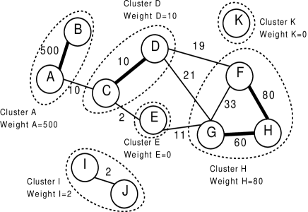
Figure 3: Clustering mechanism according to the number of roaming events between access points (with $k=0.5$).

We repeat the clustering process until there are no more links to be considered. An example of a resulting clustered graph representation is illustrated in Fig. 3. One can notice that the costs $l_{DF}$ and $l_{DG}$ are not sufficient to merge both clusters. The same happens with $l_{AC}$, $l_{CE}$, and $l_{EG}$. Such an approach serves to differentiate paths from locations where an node stays longer.

We can now define that within a cluster, an eligible locator will be the mesh router with the greater cumulated association duration to interpret the likelihood to be associated on a particular AP.

3.2.3 Resulting properties

Figure 4: CDFs of the completeness level of the resulting embedded graphs and the gathering level.

We study the variations of two important properties of the resulting embedded graphs generated through our clustering algorithm among the patterns of mobility of the nodes (see Fig. 4). We ran the clustering algorithm on 4 weeks by using $k=0.5$ on 4,766 active nodes.

The gathering level. We define as “gathering level” the ratio of the number of generated clusters on the total number of visited APs. For 68% of the nodes, the ratio is greater than $0.5$ and strictly inferior to 1, while for 23% the ratio is equal to $1$. The clustering algorithm thus performs well as it gathers mostly APs involved in ping-pong effects and high micro-mobility highlighting the different places of association.

The completeness level. We define as “completeness level” the ratio of the number of edges between the clusters on the number of edges required to obtain a complete graph. A graph of $n$ vertices is complete when there is an edge between every pairs of distinct vertices. This represents $\frac{n(n-1)}{2}$ edges. With this ratio, we have an idea of the closeness of the different clusters according to the mobility of the nodes. 22% of the nodes have a ratio equal to $0$. They do not have inter-clusters mobility and/or have only one generated cluster. In contrast only 10% have a ratio equal to $1$ which represents a limited coverage area of mobility. Finally 58% of the nodes have a ratio comprised between $]0,32]$. They have inter-cluster mobility but not completely connected graphs.

3.3 Persistence of cyclic behaviors

Otiy relies on notions of persistence of cyclic behaviors and preferential time of attachment to specific areas. In this section, we analyze patterns of association with the above-created clusters. To do so, we rewrite each movement file by replacing APs’ identifiers by their corresponding clusters’ identifiers and by aggregating the timestamps of consecutive associations in the same cluster.

3.3.1 Cyclic time-related (re)association behavior

Individuals which have habits in an environment, show cyclic patterns of mobility at the topological level. We asset this aspect through the analysis of the re-associations at prevalent locations in an hourly basis by making distinction between the days of the week.

For this analysis, we enlarge the observed period to eight weeks to be sure to not be in a situation where the nodes show optimum cyclic behaviors. We define a location (cluster) as prevalent for a specific time slot if the cumulated duration of association in this location is greater than in the others locations visited during the same time slot. For a specific time slot we take into account only the nodes which have been associated the preceding week of activity in the same time slot. Finally, each day are defined through 24 time slots of one hour each.

Figure 5: Percentage of nodes which have been associated to the same prevalent location of the week before during the same time slot.

In the Fig. 5, we analyze the persistence of the prevalence of a predicted location for each time slot by making the distinction between the days. This persistence is analyzed, each time, through two consecutive weeks of activity. We plot the percentage of nodes for which the analysis of the time slots have been possible.

From this figure we can make three main observations: (i) from weeks to weeks, the percentage of correct predictions stays approximately high and stable between 75 and 95%. (ii) The differences between the days are not strong and denote that making the distinction between the days does not affect the accuracy of the predictions. (iii) The percentage of nodes which have correct predictions is minimal in diurnal periods between (in average 75%) and maximal the nights (in average 90%). This is because we have more observed nodes during diurnal periods than in nights. The increasing number of nodes and their high activity in diurnal periods decreases sensibly the results.

However, this figure does not give information on the correctness prediction of the intra-day sequence of prevalent locations as we consider each time slot independently. We thus consider that through the scheme 1 (the expanding of location prevalence in the following empty slot) and changes in pattern of mobility, that the accuracy of the predictions will slightly decrease.

3.3.2 Persistent periods of activity

As mentioned in Section 2.2, the period of activity is a node-related parameter. In this subsection, we analyze the differences among the nodes and the persistence of this parameter.

In the following, we provide results about nodes which present a certain consistency in their activity in the network. For instance, results about mobility patterns every Monday are based on the nodes who were active the four Monday of the observed period. In the same way, weekly results are based on nodes who were active each day of at least one week. The constraint about the consistency in the activity is mostly motivated by the necessity to compare patterns of mobility on a same plan, and to be able to analyze persistence in behaviors.

Figure 6: Different types of periods of activity. It shows the results for two nodes on Monday of each week of our observed period.

The Fig. 6 presents the periods of activity of two different nodes for the same day (Monday) of the four weeks. In this figure, we analyze the behavior of the nodes within one particular day. While for the node at the left we can observe regularity in the period of non activity (between 9h and 17h), the periods of activity of the node at the right are completely different. The main important aspect is in the regularity and so the persistence of the period of activity of the node at the left. For the node at the right, the cumulated periods of activity represents approximately an activity all the day. This is an entirely different behavior which let suppose that the node can have access to the network at any time.

If these two patterns of activity can be classified in two different categories, it should exist two more different categories in this classification: (i) nodes active along the day and (ii) nodes active only during work hours. Under this classification, it is different ways for different needs which can dictate the behavior of the nodes in the access of the network. This supposes persistence at short and average terms of the behaviors. However, we can not conclude on this intra-day behavior without comparing with the periods of activity the others days of the week.

Figure 7: For each day, the CDF of the length of time slots where the nodes have never been active.

The Fig. 7 represents, for each day, the CDF of the maximum consecutive duration of non activity in the network. For each day, the periods of activity of the four weeks are cumulated to give the periods of non activity. Then the durations of non activity observed correspond to periods where the nodes have never been active in the network. The first observation is that around 40% of nodes are active all the day for every week days and 48% to 70% the week-end. The second observation is that for 60% of nodes the maximum consecutive period of non activity is nearly the same for each day of the week days except for the Fridays. 40% of these nodes is, for 12 hours and less, absent from the network.

It is important to note that the durations of non activity are clearly different between the week days and the week-end. The nodes which are subject to constraints (social or not) the week days are more free to access the network differently the week-end.

To summarize, the nodes can have cyclic periods of activity which can be for a majority of them persistent. These behaviors are not directly correlated from one day to another. It is thus required to take each day independently.

4 Evaluation

As explained previously, a locator is assigned to each time slot. To generate an agenda, each mobile node first determines for each time slot what is the prevalent cluster. At the end of the validity period of its agenda, it schedules the new locators’ positions. For each time slot, the locator is positioned in the prevalent cluster. To evaluate the accuracy of our predicted agenda, we need to check for each time slot whether the mobile node was close to its locator. Therefore we verify if the mobile node has visited its locator’s cluster during the given time period.

4.1 Methodology

For this evaluation we enlarge the period of analysis. It starts now from the 6th of January 2003 (timestamp 1041829200) to finish the end of the 29th of February 2004 (timestamp 1078117200). We choose this period length to see how the learning step can improve the accuracy of our predictions after each school holidays and with the arrival of new nodes.

To evaluate the pertinence of our agenda, we check whether the mobile node has visited its locator’s cluster during a time slot. If we find a match, we consider the mobile node is effectively close to its locator. We perform this comparison for each time slot, each time a mobile node was connected to the network at least once during a time slot. We do not consider time slots where a node is inactive. Similarly, we do not include in our study the reliability of the first bootstrapped agenda, as it does not reflect an observed mobility pattern. The creation of the first agenda is detailed in Section 2.3.2.

For each time slot, we can thus define a good or a bad prediction. We evaluate the accuracy of the agenda as the ratio of bad predictions ($NbBadPredictions$) over the total number of considered time slot ($TotalNbSlots$). We define the error of prediction in the agenda as $A_{er}$ by:

$$A_{er}=\frac{NbBadPredictions*100}{TotalNbSlots}.$$

W.l.g, we choose to update, each week and for each node the clusters by taking into account the recent patterns of mobility but also all the preceding history of patterns of mobility. The update of the clusters is made after the agenda evaluation and we make sure that the preceding locator predictions are still correct even if the eligible locators for the clusters have changed.

4.2 Evaluation of the $A_{er}$

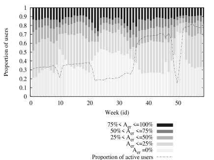
Figure 8: Histogram of the proportion of nodes according to their $A_{er}$ for each week.

For each week in Fig. 8, we plot the histogram of the proportion of nodes which have an $A_{er}$ value of 0% (perfect prediction), less or equal to 25%, 50%, 75% and 100%. We used a minimum of one week and up to two weeks of mobility history to predict the value of the agenda.

The first observation is the large proportion of nodes having an accurate agenda for the all week, $A_{er}=0\%$. Peaks of this phenomenon can be observed at summer breaks or during Christmas holiday. This certainly results from a static behavior of nodes. This proportion increases as the number of active node decreases.

We also observed that only around 40% of the average proportion of nodes have at least 25% of incorrect predictions in their agenda. Depending on the observed week, this proportion of nodes varies between 20 and 50%. An average of 15% of the proportion of nodes have more than 75% of wrong predictions in their agenda and approximately 10% have between 50% and 75% of bad accuracy.

It is important to note that if a node is not active during a time slot, a default locator is set in the agenda, thus repeating the value of the previous locator as explained in Section 2.3.1. A bad prediction can be easily explained by a lack of information about a node mobility pattern. This phenomenon can be observed in the Fig. 8, when the proportion of active nodes increases and remains stable (marked as a line on the plot). We can note that the persistence of the patterns of mobility then improves the accuracy of the generated agenda. This accuracy decreases logically at the beginning and at the end of the different holidays periods as mobility constraints are relaxed during holidays and new nodes join the network.

In facts, the reasons of most of the wrong matches are simple: (i) often, nodes active only two weeks in the observed period do not develop any cyclic pattern of mobility and thus have an high $A_{er}$ value. (ii) More rarely, places which certainly constitute part of a path between two significant areas are assigned to time slots (through scheme 1). Finally, (iii) overlapping between prevalent places for one node occurs most of the time between 9am and 3pm.

These first results appear extremely promising for Otiy, our location scheme, as it give in much cases an agenda that can allow the optimization of the localization process.

4.3 Impact of the history length

Figure 9: Impact of history length used to generate the agenda on the number of correct matches ($A_{er}\leq 50\%$).

In the Fig. 9, we analyze the contribution of the length of mobility history used to create the agenda on the percentage of correct matches. Here, we plotted only the case where there are up to 50% bad matches in the agenda prediction.

We get the higher proportion of nodes having at least 50% of the time a good estimation of their agenda prediction for a mobility history of one week. This means that recent mobility patterns are sufficient to estimate an accurate agenda. Nevertheless, the duration of activity during the current and preceding weeks also has a clear impact on the $A_{er}$.

A convergence between different length of history can be observed after as a result of more stable behavior of nodes. But using long mobility history, one can note that the agendas appears more sensitive to changes of mobility patterns. On the figure (week 11, weeks 20 to 23, and weeks 32 to 35), we clearly see that the accuracy of the agendas drop roughly at the beginning and the end of the school holidays period.

In order to get an agenda reactive to the changes of mobility pattern but also be able to gather enough data about nodes’ behavior to get the right locator estimate, we choose in the rest of our tests to use at a two weeks mobility history.

4.4 Comparison between the different days

Figure 10: Proportion of the nodes which have an $A_{er}\leq 50\%$ for each day.

It is interesting to check whether the mobility behaviors affect differently the percentage of incorrect predictions depending particular week days. In the Fig. 10 we compare the proportion of nodes which have an $A_{er}\leq 50\%$ for each day of the week.

The first observation, is that the proportion of nodes with the same accuracy in their agenda remains approximately the same whatever day is considered (between 70 and 90%). However, the variations of proportion are more pronounced for week-ends and Mondays. These days are more sensitive to changes in nodes’ behavior at the beginning and at the end of the holidays. The rest of the time the pertinence of the agenda seems more important for these three days.

We envision taking advantage of this phenomenon to better detect changes in behaviors and to more accurately restart the bootstrapping procedures.

4.5 Evaluation of the physical distance

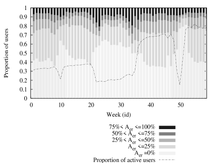
Figure 11: Histogram of the proportion of nodes according to their $A_{er}$ values for each week. In this figure, we consider also a correct prediction if the node has visited at least one cluster connected (at one hop) to the locator.

As mentioned before, the topology of the network is not provided with the data traces. As a consequence we can not determine the topological path length(s) between the visited areas during a time slots and the locator’s position.

In order to have an idea of how close the nodes have been from the locator’ cluster, we use the graph from which is built the clusters. In the Fig. 11, we evaluate $A_{er}$ considering a prediction as correct, if during a time slot, a node has visited the locator’ cluster until a cluster one hop away.

Comparing the results with Fig. 8, we observe that the number of nodes with an $A_{er}$ value of up to 50% of their agenda increases roughly by 10% for each week. The number of nodes which have made more than 75% of incorrect predictions is reduced to, in average, 5% per week.

These results show, that for the majority of the nodes and most of the time we successfully provide a locator close to the current physical location of the nodes. We therefore can provide an agenda that satisfactory reflects nodes mobility.

5 Related Work

The problematic of reducing the amount of generated location updates in a wireless network has been well studied in PCS and is very close to our work. Even if the proposals are not really adapted to IEEE 802.11 wireless mesh networks, we will relate the different concepts of the most relevant work.

Tabbane is one of the firsts to have introduced the node (mobility) profiling to improve location management in PCS. In [14] the profiling is operated by the network and shared with the node’s subscriber identity module SIM. Thanks to this profiling, whatever the period of time $[t_{i},t_{j})$ the system can find a list of areas where the nodes could be. This list of areas is decreasingly ordered by the probabilities of being in the different areas. One probability is dependent of a function associated with and has several parameters such as the time, the pattern of mobility, the last location, the weather etc. Until the node is in one of these areas it does not update its location. When the system needs to locate him, it asks sequentially the different areas within the list. Two notions are shared with our approach: (i) the node profiling although in Otiy it is the nodes which make their self-profiling. (ii) The relation with the time. However, in Otiy the period of time are predefined and only one area (anchor) is assigned to each time slot.

Chuon et al. in [3] by calculating the prevalence of the daily different visited cells create an node profile graph (IPG) per node and through their monitoring by the network. This graph is composed by vertices (cells) where the normalized probability of visit on N-days is greater than a specified value (comprised between $0$ and $1$) and the connectors between these cells (also called anchors). Furthermore, the vertices in the IPG are classified by decreasing order of probability of visit. Until the node stays in the set of vertices in his IPG it does not have to updates its location. To locate it in its IPG, the network pages it in the decreasing order of probability of the anchors as in [11]. We differ from this approach in several ways. We do not cumulate daily patterns of mobility to see a prevalent mobility graph. Rather, we distinguish each daily pattern of mobility of the week to capture the different constraints and interests which are dependent of the days. Although they used the division in time slots to prove that their IPG captures well the diurnal mobility of the nodes, they do not used these time slots to make the relationship, that we make, between a particular area and the time. From this point, our proposal is clearly different of the methods used to updates the locations and to page the nodes.

In [16], Wu et al. mine the mobility behavior nodely (operated by the nodes) from long term mobility history. From this information they evaluate the time-varying probability of the different nodely-defined regions. The prevalence of a region on the time is defined through a cost model. Finally, they obtain a vector $<time,area>$ of mobility which will define the region to be paged in function of the time. The location updates and paging schemes are approximately the same than the afore-presented proposals. Here, the prevalence of a particular area on the time is more flexible and accurate than ours. However, the complexity of the algorithm is more important. Furthermore, the length of the vector of mobility can be a lot more important than a division in time slots of equal duration.

Finally in IEEE 802.11 wireless networks, Ghosh et al. have profiling the nodes associations sequences by making the difference between the days in [5]. The result is several patterns of mobility such as Weekend Profile, Home Profile, etc. Here, the areas are called “sociological hub” and are defined at a building granularity. With this set of profiles they are capable to determine which mobility profile the node follow currently (from the firsts associations) and/or define a window of day with attributed mobility profiles. This approach is sensibly different of Otiy but here, we recognize the necessity to differentiate the patterns of mobility which could be different from day to day. Furthermore, our significant areas (they “hub”) are determined by the local micro-mobility of each node and are not based on any geographical information (e.g., building segmentation).

6 Conclusion

We introduced Otiy, a node-centric architecture to control the propagation of the location updates in networks of mobile nodes. To limit the impact of location updates, each node creates an agenda of locators, which are access points at which the node will probably get associated with according to the past and present patterns of mobility. The idea behind this approach is to make location update overhead more localized.

The keys principles we achieve are:

• A fully decentralized location service.

• Short path lengths for location updates.

• Shared knowledge on absolute time locations. At anytime, both the node and its interlocutor(s) know the location of the locator.

To achieve our goals, we proposed to gather nearby APs in terms of node roaming events in order to create areas (clusters) of micro-mobility. Our clustering algorithm does not use any geographical information and is based only on the sequence of associations/disassociations. This drastically limits the propagation of updates due to artifacts such as ping-pong effects.

Using around one year of mobility traces, we have in average 75% of the nodes that have at least 50% of their time slots which match exactly the right predictions. These results encourage us to keep improving Otiy and evaluate it using real testbeds.

References

- [1] M. Balazinska and P. Castro. Characterizing mobility and network usage in a corporate wireless local-area network. In Proc. of MobiSys 2003, pages 303–316, San Francisco, CA, May 2003.
- [2] C. Cheng, H. Lemberg, S. Philip, E. van den Berg, and T. Zhang. Slalom: A scalable location management scheme for large mobile ad-hoc networks. Wireless Communications and Networking Conference, 2:574–578, 2002.
- [3] C. Chuon, S. Guha, and A. K. M. M. Hossain. Individual profile graphs for location management in pcs networks. Wireless Networks, Communications and Mobile Computing, 2005 International Conference on, 1:187–192, June 2005.
- [4] J.-M. François and G. Leduc. AP and MN-centric mobility prediction: A comparative study based on wireless traces. In Proc. of IFIP Networking 2007, pages 322–332, Atlanta, GA, USA, May 2007.
- [5] J. Ghosh, M. J. Beal, H. Q. Ngo, and C. Qiao. On profiling mobility and predicting locations of campus-wide wireless users. In Proc. of the second international workshop on Multi-hop ad hoc networks: from theory to reality, Florence, Italy.
- [6] T. Henderson, D. Kotz, and I. Abyzov. The changing usage of a mature campus-wide wireless network. In Proc. of the Tenth Annual International Conference on Mobile Computing and Networking (MobiCom), pages 187–201, Philadelphia, PA, USA, 2004.
- [7] J. P. Hubaux, T. Gross, J. Y. L. Boudec, and M. Vetterli. Towards self-organized mobile ad hoc networks: the Terminodes project. IEEE Communications Magazine, 31(1):118–124, 2001.
- [8] G. L. Jean-Marc François and S. Martin. Learning movement patterns in mobile networks: a generic method. In European Wireless 2004, Barcelona, Spain.
- [9] D. Kotz, T. Henderson, and I. Abyzov. CRAWDAD trace dartmouth/campus/syslog/01 04 (v. 2004-12-18), dec 2004.
- [10] D. Kotz, T. Henderson, and I. Abyzov. CRAWDAD trace set dartmouth/campus/movement (v. 2005-03-08), March 2005.
- [11] G. P. Pollini and C.-L. I. A profile-based location strategy and its performance. IEEE Journal on Selected Areas in Communications, 15(8):1415–1424, 1997.
- [12] L. Song, D. Kotz, R. Jain, and X. He. Evaluating location predictors with extensive wi-fi mobility data. In Proc. of the 23rd Annual Joint Conference of the IEEE Computer and Communications Societies (INFOCOM), volume 2, pages 1414–1424, 2004.
- [13] I. Stojmenovic and B. Vukojevic. A routing strategy and quorum based location update scheme for ad hoc wireless networks, 1999.
- [14] S. Tabbane. An alternative strategy for location tracking. IEEE Journal on Selected Areas in Communications, 13, Issue 5:880–892, June 1995.
- [15] S.-C. M. Woo and S. Singh. Scalable routing protocol for ad hoc networks. Wireless Networks, 7(5):513–529, 2001.
- [16] H.-K. Wu, M.-H. Jin, and J.-T. Horng. Personal paging area design based on mobiles moving behaviors. In INFOCOM, pages 21–30, 2001.
- [17] J. Zhang and L. Gruenwald. Spatial and temporal aware, trajectory mobility profile based. In Proc. of The International Database and Expert Systems Applications (DEXA) Workshop on Mobile Database and Distributed Systems, pages 716–720, September 2002.