A systematic expansion for relativistic causal hydrodynamics

Abstract

A systematic expansion of the Boltzmann equation for the diffusion of dilute tracers, in powers of the Knudsen number, carried out to next-to-leading order (NLO), gives the relativistic causal diffusion equation (Kelly’s equation). Using dimensionless combinations of dynamical quantities, we show when the small NLO term plays a crucially important role. We proceed to show that a derivation of Kelly’s equation from a microscopic theory of the correlation function of the number density of diffusers is possible. The correlator fulfils the Green-Kubo relation for the diffusion constant, as well as an f-sum which goes beyond a purely phenomenological causal theory. We argue that the construction generalizes to the full hydrodynamic equations.

After Eckart eckart and Landau landau cast Navier-Stokes hydrodynamics into manifestly Lorentz covariant form, it was realized that there still remained an essential acausality in the theory acausal ; kelly . The problem was solved in principle by Israel and Stewart causal who wrote down a phenomenological theory which has since been applied to heavy-ion collisions, the quintessential laboratory for ultra-relativistic hydrodynamics hic . The hydrodynamic equations are obtained by making a derivative expansion of the transport equations. If the longest microscopic time scale in the problem is a relaxation time $\tau_{R}$, then the hydrodynamic equations are valid for times, $\tau\gg\tau_{R}$. When the Knudsen number, $K=\tau_{R}/\tau$, goes to zero, the microscopic origin of the theory is effaced and what remains is a continuum theory. The usual equations of hydrodynamics are obtained in this way at leading order (LO) in $K$, i.e., at ${\cal O}(K^{0})$ grad . Here we discuss the version of the equations which appears at the next-to-leading order (NLO) in $K$.

Two questions seem not to have been addressed fully in the literature, and are interesting enough that we consider them briefly here. The first question is the following: is the restoration of causality at NLO necessary, or is it an accident? The second question is: given a correlation function computed from the underlying microscopic theory, how does one show that the causal relativistic hydrodynamic theory is obtained at late times? We examine these questions here for the simplest of hydrodynamic equations— the diffusion equation, and its causal version: Kelly’s equation. The answers are generalizable to all hydrodynamic equations, as we argue.

Recall that the continuity equation for the density, $n$, of a dilute tracer inserted into a thermalized background fluid,

$$\frac{\partial n(\mathbf{x},t)}{\partial t}+\nabla\cdot\mathbf{J}(\mathbf{x},t)=0,$$ (1)

where $\mathbf{J}$ is the tracer current, expresses conservation of the number of tracer particles. Putting this together with the phenomenologically established Fick’s law,

$$\mathbf{J}(\mathbf{x},t)=-D\nabla n(\mathbf{x},t),$$ (2)

where $D$ is called the diffusion constant, gives rise to the diffusion equation,

$$\frac{\partial n(\mathbf{x},t)}{\partial t}=D\nabla^{2}n(\mathbf{x},t).$$ (3)

$D$ is an example of a transport coefficient. A comparison of the strength of the two terms in the equation yields a dimensionless variable which we call the Wiener number,

$${\cal W}=\left(\frac{\partial n}{\partial t}\right)\biggm{/}\left(D\nabla^{2}n\right)=\frac{L^{2}}{\tau D},$$ (4)

where $\tau$ is the time and $L$ the distance over which the diffusion phenomenon is observed. For typical diffusive behaviour we expect ${\cal W}$, to be finite, non-zero, and constant in time, which yields the familiar result $L\simeq\sqrt{D\tau}$. This violates relativistic causality for $\tau<D{\cal W}/c^{2}$, since $L>c\tau$ in that case. This is shown in Figure 1. One suspects that the diffusion equation is not valid at very early times, but there is nothing in the equation that prevents this. As is well-known, the local conservation equation (eq. 1) obeys relativistically causality. As a result, its violation in the eq. (3) can be traced to Fick’s law.

Kelly kelly examined the Boltzmann transport equation for the distribution function of a dilute gas of tracer particles in the background of a thermal gas in equilibrium. The transport theory is assumed to satisfy relativistic causality. The condition that the background gas has no flow selects out a special frame in which the gas is at rest. In the remainder of this note we work in this frame, giving up manifest Lorentz covariance for notational ease. The diluteness aproximation is used to retain only linear terms in the tracer density inside the collision integral. The collision term then yields up a natural microscopic scale of time through the collision frequency, $\nu=1/\tau_{R}$.

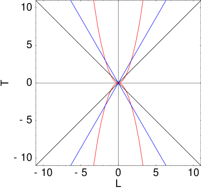
Figure 1: The parabola is a locus of constant $\cal W$ and contains the diffusive wake. The sets of straight lines are loci of constant $M^{2}$ (the inner set for $M=1$, and the outer for $M=1/c_{s}$, i.e., the light cone) and denote the causal front. The lack of relativistic causality of the diffusion equation is seen in the fact that the parabola lies outside the light cone at small $\tau$. For any $M$, the front and wake can be distinguished at late times.

It was shown that the expansion carried out to order $K$ yielded the hyperbolic diffusion equation—

$$\tau_{R}\frac{\partial^{2}n}{\partial t^{2}}+\frac{\partial n}{\partial t}=D\nabla^{2}n,$$ (5)

and, an expression for the diffusion constant,

$$D=\tau_{R}c_{s}^{2},$$ (6)

where $c_{s}^{2}$ is the RMS velocity of the tracer particles. Explicit solutions of the differential equation with this subsidiary condition show that relativistic causality is restored kelly .

The relative importance of the causal (the second derivative in energy) and the frictional terms (the first derivative) is given by the dimensionless ratio

$$\left(\tau_{R}\frac{\partial^{2}n}{\partial t^{2}}\right)\biggm{/}\left(\frac{\partial n}{\partial t}\right)\simeq\frac{\tau_{R}}{\tau}=K.$$ (7)

This is exactly as expected, since the causal term arises at NLO in $K$, and one obtains the diffusion equation by neglecting it. The relative importance of the causal term and the force is

$$M^{2}=\left(\frac{\tau_{R}}{D}\right)\,\left(\frac{\partial^{2}n}{\partial t^{2}}\right)\biggm{/}\bigl{(}\nabla^{2}n\bigr{)}\simeq\left(\frac{L}{c_{s}\tau}\right)^{2}.$$ (8)

Phenomena occurring at constant $M^{2}$ would include a causal diffusive front propagating with speed $V=L/\tau$. Thus $M$ is the diffusive analogue of the Mach number. The three dimensionless constants are not independent, since, by construction, $M^{2}=K{\cal W}$.

The existence of a non-vanishing scale $\tau_{R}$ allows restoration of relativistic causality. On the light cone one has $L=c\tau$. The locus of constant $\cal W$ lies completely inside the light cone for a $\tau_{*}$ given by $\sqrt{{\cal W}D\tau_{*}}\leq c\tau_{*}$. A little manipulation using the expression for $D$ in eq. (6) brings this to the form $K_{*}=\tau_{R}/\tau_{*}\leq M_{c}^{2}/{\cal W}$, where $M_{c}$ is the value of $M$ when $V=c$ and $K_{*}$ is the value of $K$ at which causality is restored. One may note, with kelly , that for $\tau<\tau_{*}$ the frictional term in eq. (5) can be neglected, so that using eq. (6), the remaining terms become a wave-equation. Since $c_{s}^{2}<c^{2}$, relativistic causality is restored. More correctly, one notes that in the problematic region $K>K_{*}\simeq{\cal O}(1)$, and hence the expansion breaks down. Thus, causality is restored by shielding the problematic region from the continuum equation. Investigation of $\tau<\tau_{*}$ must be carried out in transport theory, which is causal by construction.

In kelly it was noted that the solutions of eq. (5) consist of two distinct regions— the “wake”, i.e., $L\propto\sqrt{\tau}$, where characteristic diffusive behaviour is seen, and the “front”, i.e., $L\propto\tau$, where causal behaviour is restored. This is precisely the result of our analysis here (see Figure 1). The wake is characterised by the physics of fixed $\cal W$, and the front by fixed $M$. $\cal W$ is, of course, inherent in the continuum theory. The appearance of a new, non-vanishing, dimensionless constant $K$ implies the existence of a new constant $K{\cal W}$, which leads to a shielding of the acausal region, as discussed above. This answers our first question: the restoration of causality is a necessary consequence of the NLO expansion in $K$.

This analysis also tells us when to use Kelly’s equation rather than the usual diffusion equation. Clearly, at late times, the differences between the two are minor in the region of the wake. The strength of the front decays exponentially in $1/K$ kelly , so this is also negligible at late times. At late times, therefore, the physics of the two equations is identical. Kelly’s equation is to be used at early times, as the above analysis of causality shows. The two equations give different results at times when the front and the wake have not clearly separated. However, it is useful to be aware of the fact that at such times higher order effects, or the full Boltzmann equation, could be needed.

We turn next to the second question and explore the relation between correlation functions and the hydrodynamic equation $Ln=0$, where $L$ is a differential operator in space-time. Although the computation is classic textbook material forester , the connection with relativistic causal hydrodynamics has not been noted. The linear response function, i.e., the expectation value of the retarded density-density correlator, $\chi$, is given by

$$\chi(k,z)=\chi(0,0)\left[1+izG(k,z)\right],$$ (9)

where $z$ is a complex frequency in the upper-half plane, $k$ a spatial momentum, and $G(k,z)$ is the Green’s function, i.e., inverse of the operator $L$ forester . For the diffusion equation one has

$$G(k,z)=\frac{i}{z+iDk^{2}}\qquad{\rm hence}\qquad\chi(k,z)=\frac{iDk^{2}\chi(0,0)}{z+iDk^{2}}.$$ (10)

The spectral density is the limit as $k\to 0$ of the imaginary part of $\chi/k^{2}$ as $z$ approaches the real line from above. Hence, for the diffusion equation one finds that

$$\sigma(\omega)=\frac{D\chi(0,0)}{\omega}.$$ (11)

This is the basis for the Green-Kubo formula

$$D\chi(0,0)=\stackrel{{\scriptstyle lim}}{{\scriptscriptstyle\omega\to 0}}\omega\sigma(\omega).$$ (12)

Given any microscopic theory (for example, a quantum field theory specifying the interactions between the tracer particles and the constituents of the background fluid) which enables one to compute the spectral function, $\sigma(\omega)$, the diffusion equation can be obtained if $\omega\sigma(\omega)$ has a finite limit as $\omega$ vanishes. The Green-Kubo relation, along with the positivity of $\omega\sigma$, provide a derivation of the diffusion equation from the microscopic theory. In a complete microscopic computation, the moments of the spectral density also exist. Since, the spectral density of the diffusion equation does not have well-defined moments, the diffusion equation does not care for these details.

A straightforward treatment of Kelly’s equation runs into subtleties. From eq. (5) one sees that

$$G(k,z)=\frac{i}{-i\tau_{R}z^{2}+z+iDk^{2}},\qquad{\rm hence}\qquad\sigma(\omega)=\frac{D\chi(0,0)}{\omega(1+\omega^{2}\tau_{R}^{2})}\times\stackrel{{\scriptstyle lim}}{{\scriptscriptstyle k\to 0}}\left[1-\frac{\tau_{R}\omega^{2}}{k^{2}D}\right].$$ (13)

Since the last factor diverges except for constant $M^{2}=\tau_{R}\omega^{2}/Dk^{2}$, there seems to be no sensible spectral function otherwise. One could either proceed with caution along curves of constant $M^{2}$, or use a regulator.

The text-book regulator is the memory kernel method forester . One delays the response of a system to a disturbance by introducing the memory kernel—

$$\mathbf{J}(\mathbf{x},t)=\int_{0}^{t}dt^{\prime}D(t-t^{\prime})\nabla n(\mathbf{x},t^{\prime}),\qquad D(t-t^{\prime})=-\frac{D}{\tau_{R}}\exp\left(\frac{t^{\prime}-t}{\tau_{R}}\right).$$ (14)

where the explicit expression for the memory kernel above constitutes the relaxation time ansatz. Putting this together with the continuity equation, one finds

$$G(k,z)=\frac{i}{z+iDk^{2}/(1-iz\tau_{R})},\qquad\chi(k,z)=\frac{iD\chi(0,0)k^{2}}{z+iD(k^{2}-z^{2}\tau_{R}/D)},\qquad\sigma(\omega)=\frac{D\chi(0,0)}{\omega(1+\omega^{2}\tau_{R}^{2})}.$$ (15)

Note that this spectral function is perfectly regular as $k\to 0$. Our earlier analysis of dimensionless combinations of variables is also reflected in this spectral function. To recover the diffusion equation, the spectral function in (eq. 11) must be accurate for arbitrarily small $\omega$; so this is the limit $K\to 0$. The new term in the Green’s function in eq. (15) is a correction to the diffusion equation to NLO in $K=\omega\tau_{R}$. Although the extra terms are parameterically small in $K$, they have important effects when $M\ll 1$ is constant. These effects arise at $\omega\propto k$, which is precisely the region at which causal effects manifest themselves.

Since $\omega\sigma(\omega)$ is positive and the Green-Kubo formula is obeyed for $M\ll 1$, this is an acceptable description of diffusion. The analysis is completed by noting that eq. (14) implies that Fick’s law must be replaced by the generalization

$$\left[1+\tau_{R}\frac{\partial}{\partial t}\right]\mathbf{J}(\mathbf{x},t)=-D\nabla n(\mathbf{x},t),$$ (16)

which gives the NLO correction in $K$ to the left hand side. Eliminating $\mathbf{J}$ between the continuity equation (eq. 1) and the above relation then yields Kelly’s equation (eq. 5), as noticed in mota . A phenomenological theory, such as eq. (16), leads to Kelly’s equation. However, such a theory would have two material constants, $D$ and $\tau$, whereas the microscopic theory has only one.

While the Green-Kubo formula provides the correct reduction of the microscopic theory to the continuum, the spectral function in eq. (15) contains more. Its first moment exists, and $\langle\omega\rangle=D/\tau_{R}$. Through Fourier transforms, the moments of the spectral function are related to time derivatives of the imaginary part of the linear response function, $\chi^{\prime\prime}(\mathbf{x},t;\mathbf{x}^{\prime},t^{\prime})=\langle[n(\mathbf{x},t),n(\mathbf{x}^{\prime},t^{\prime})]\rangle/2$, where $n$ is the number operator in the microscopic theory. Each time derivative on $n(\mathbf{x},t)$ becomes a commutator with the Hamiltonian. For the first moment, the double commutator is a generalization of the f-sum rule (also called the Thomas-Reiche-Kuhn sum rule) of atomic physics, and can be written as

$$\frac{1}{\chi(0,0)}\int\frac{d\omega}{2\pi}\omega\sigma(\omega)=i\int d\mathbf{x}\left\langle[[n(0,t),H(0,t)],n(\mathbf{x},t)]\right\rangle.$$ (17)

A straightforward computation of the right hand side then leads to $D/\tau_{R}=\langle v^{2}\rangle$, the RMS velocity, and reproduces eq. (6) for the diffusion constant. The f-sum rule knows about the microscopic constituents through the right hand side of eq. (17), and hence can be used to constrain models. As an example, note that the fluctuation-dissipation theorem gives $2mT=D/\tau_{R}$, where $T$ is the temperature and $m$ the mass of the diffuser. For heavy quarks, such as the charm or bottom, one would expect that a computation of $\tau_{R}$ would immediately yield $D$ through this relation. For diffusion of quantum numbers dominated by light quarks, such as the baryon number or electric charge, where the effective mass of the carriers is unknown, this relation potentially gives new information. Higher analogues of the sum rule exist at higher orders in $K=\omega\tau_{R}$. Keeping successively higher moments, one can construct successively higher order terms in the analogue of Fick’s law. This is a construction of effective dynamical theories at different time scales. Our second question is now answered.

Finally we consider whether this analysis can be extended to full hydrodynamics. The major difference between the diffusion and Navier-Stokes equations is that the latter are non-linear. In the continuum limit, $K\to 0$, all hydrodynamic equations can be derived by combining three kinds of equations: continuity equations (such as eq. 1) which relate a density and its current, constitutive equations (analogues of Fick’s law) which relate the current to the density through a transport coefficient, and thermodynamic relations of various kinds, which serve to eliminate redundant variables. Non-linearities arise through the fact that the constitutive equations contain terms in powers of the velocities. However, the dissipative terms are constructed to be linear, and therefore the essential features discovered here in the diffusion equation generalize to hydrodynamics.

Corrections to the continuum limit, in the form of NLO terms in $K\ll 1$ can then be expected to yield results similar to those we have obtained for the diffusion equation mota . In particular, the memory kernel method is expected to give correction terms to the constitutive equations similar to eq. (16). As a result, the corrections to the hydrodynamic limit of the spectral function will be similar to those encountered in eq. (15). All these arguments generalize, and the NLO corrections to the hydrodynamic equations are always expected to restore causality. In addition, the Green-Kubo formulae for the transport coefficients are not modified— a matter of some importance for the computation of transport coefficients from QCD using weak-coupling methods, lattice computations or the AdS/CFT correspondence. The NLO corrections in $K$ give rise to a connection between the relaxation time and transport coefficient through an f-sum rule. Since the f-sum rule constrains the microscopic degrees of freedom, they can be valuable in interpreting results obtained from lattice or AdS/CFT techniques. Such a systematic microscopic derivation of the hydrodynamic equations improves upon the Israel-Stewart formulation by relating various new material constants to the old ones through the f-sum rules.

In conclusion, the systematic expansion of transport theory in the Knudsen number, $K$, which gives the usual hydrodynamic theory to LO in $K$, i.e., at ${\cal O}(1)$, lacks relativisitic causality at early times acausal ; kelly . This acausal region is necessarily shielded at next to leading order in $K$, i.e., at ${\cal O}(K)$ through the generation of a time scale, $\tau_{R}$, and the breakdown of the equations for $\tau\simeq\tau_{R}$. Phenomenological theories can give the same causal hydrodynamic equations as the NLO expansion while introducing seemingly new material constants. The systematic expansion in $K$ relates the new constants to the usual transport coefficients through f-sum rules. An order-by-order matching of any microscopic computation of a correlation function to the hydrodynamic equations is possible, and can be seen as the construction of successive effective long-time theories.

I would like to thank Rajeev Bhalerao and Jean-Yves Ollitrault for discussions, and IFCPAR project 3104-3 for making the latter possible.

References

- (1) C. Eckart, Phys. Rev., 58, 919, (1940).
- (2) L. D. Landau and E. M. Lifshitz, Fluid Mechanics, Elsevier, New Delhi (2005).
-
(3)
H. D. Weymann, Am. J. Phys., 35, 488, (1967);
N. G. van Kampen, Physica, 46, 315, (1970). - (4) D. C. Kelly, Am. J. Phys., 36, 585, (1968).
-
(5)
W. Israel, Ann. Phys., 100, 310, (1976);
J. M. Stewart, Proc. Roy. Soc., A 357, 59, (1977);
W. Israel and J. M. Stewart, Ann. Phys., 118, 341, (1979);
W. A. Hiscock and L. Lindblom, Ann. Phys., 151, 466, (1983). -
(6)
A. Muronga, Phys. Rev. Lett. , 88, 062302, (2002) and Phys. Rev. C, 69, 034903, (2004);
U. Heinz, H. Song and A. K. Chaudhuri, Phys. Rev. C, 73, 034904, (2006);
R. Baier, P. Romatschke and U. A. Wiedemann, Phys. Rev. C, 73, 064903 (2006), and Nucl. Phys., A, 782, 313 (2007);
P. Romatschke and U. Romatschke, arXiv:0706.1522;
R. Bhalerao and S. Gupta, arXiv:0706.3428. - (7) H. Grad, Phys. Fluids, 6, 147, (1963).
- (8) D. Forester, Hydrodynamics, Correlation Functions and Broken Symmetry, W. A. Benjamin Inc., Reading, MA, USA, 1975.
- (9) T. Koide, G. S. Denicol, Ph. Mota and T. Kodama, Phys. Rev. C, 75, 034909, (2007).