Yang-Mills Ground State in 2+1 Dimensions and Temporal Gauge

Abstract:

A gauge-invariant wavefunctional is proposed as an approximation to the ground state of Yang-Mills theory in 2+1 dimensions, quantized in temporal gauge. The proposed vacuum state is the true ground state of the appropriate Hamiltonian in both the free-field limit, and in a zero mode strong-field limit. Confinement, in this approach, arises via dimensional reduction, and we present numerical results for the mass gap. The issue of color screening is briefly discussed.

1 Introduction

From time to time there have been efforts [1, 2, 3, 4, 5, 6, 7, 8, 9, 10, 11, 12, 13] to obtain the Yang-Mills vacuum wavefunctional, often in lower dimensions, to see if anything can be learned about confinement and the mass spectrum. The problem is to solve for the ground state $\Psi_{0}[A]$ of the Yang-Mills Hamiltonian $H$, which has its simplest form in temporal gauge

$$H=\int d^{d}x\left\{-{\textstyle{\frac{1}{2}}}{\delta^{2}\over\delta A^{a}_{k}(x)^{2}}+{\textstyle{\frac{1}{4}}}F_{ij}^{a}(x)^{2}\right\}$$ (1)

The price for this simplicity, in temporal gauge, is that all physical states are required to satisfy a constraint

$$\Bigl{(}\delta^{ac}\partial_{k}+g\epsilon^{abc}A^{b}_{k}\Bigr{)}{\delta\over\delta A^{c}_{k}}\Psi=0$$ (2)

which enforces invariance under infinitesimal gauge transformations.

Our claim is that the ground state solution in $D=2+1$ dimensions, in temporal gauge, is approximated by

$$\Psi_{0}[A]=\exp\left[-{\textstyle{\frac{1}{2}}}\int d^{2}xd^{2}y~{}B^{a}(x)\left({1\over\sqrt{-D^{2}-\lambda_{0}+m^{2}}}\right)^{ab}_{xy}B^{b}(y)\right]$$ (3)

where $B^{a}=F_{12}^{a}$ is the color magnetic field strength, $D^{2}$ is the covariant Laplacian in the adjoint color representation, $\lambda_{0}$ is the lowest eigenvalue of $-D^{2}$, and $m$ is a constant of order $g^{2}$. In support of this claim, we will argue that (3) (i) is a solution of the YM Schrödinger equation in the $g\rightarrow 0$ limit; (ii) solves the YM Schrödinger equation in the strong field, zero-mode limit; (iii) confines if $m>0$, and that $m>0$ seems energetically preferred; and (iv) results in the numerically correct relationship between the mass gap and the string tension. A more complete report of our results can be found in a recent article [15].

2 Free-Field and Zero-Mode Limits

In the free-field $g=0$ limit, eq. (3) becomes

$$\Psi_{0}[A]=\exp\left[-{\textstyle{\frac{1}{2}}}\int d^{2}xd^{2}y\Bigl{(}\partial_{1}A^{a}_{2}(x)-\partial_{2}A^{a}_{1}(x)\Bigr{)}\left({\delta^{ab}\over\sqrt{-\nabla^{2}}}\right)_{xy}\Bigl{(}\partial_{1}A^{b}_{2}(y)-\partial_{2}A^{b}_{1}(y)\Bigr{)}\right]$$ (4)

which is the known ground state solution in the abelian, free-field case, and an obvious starting point for any investigation such as ours. Apart from the free-field limit, there is another, quite different limit which can be treated analytically. Consider gauge fields which are constant in space, but variable in time, in D=2+1 dimensions. The Lagrangian is

$$L = {\textstyle{\frac{1}{2}}}\int d^{2}x~{}\Bigl{[}\partial_{t}A_{k}\cdot\partial_{t}A_{k}-g^{2}(A_{1}\times A_{2})\cdot(A_{1}\times A_{2})\Bigr{]}$$ (5)

$$= {\textstyle{\frac{1}{2}}}V\Bigl{[}\partial_{t}A_{k}\cdot\partial_{t}A_{k}-g^{2}(A_{1}\times A_{2})\cdot(A_{1}\times A_{2})\Bigr{]}$$

with Hamiltonian operator

$$H=-{\textstyle{\frac{1}{2}}}{1\over V}{\partial^{2}\over\partial A_{k}^{a}\partial A_{k}^{a}}+{\textstyle{\frac{1}{2}}}g^{2}V(A_{1}\times A_{2})\cdot(A_{1}\times A_{2})$$ (6)

where $V$ is the volume of 2-space. With some algebra, one may verify that

$$\Psi_{0}=\exp\left[-{\textstyle{\frac{1}{2}}}gV{(A_{1}\times A_{2})\cdot(A_{1}\times A_{2})\over\sqrt{|A_{1}|^{2}+|A_{2}|^{2}}}\right]$$ (7)

satisfies the zero-mode Yang-Mills Schrödinger equation up to $1/V$ corrections. For comparison, we consider our proposed vacuum state (3) in the strong $A$-field limit, where the covariant Laplacian is dominated by the gauge-field zero-mode, i.e.

$$(-D^{2})^{ab}_{xy}=g^{2}\delta(x-y)\Bigl{[}(A_{1}^{2}+A_{2}^{2})\delta^{ab}-A_{1}^{a}A_{1}^{b}-A_{2}^{a}A_{2}^{b}\Bigr{]}$$ (8)

In this limit, it is not hard to show that $\Psi_{0}[A]$ of eq. (3) precisely reduces to (7). Thus the proposed ground state not only has the correct free-field limit, but also agrees with the calculable ground state of the zero-mode Schrödinger equation in an appropriate strong-field limit.

3 Dimensional Reduction and Confinement

A long time ago it was suggested [1] that at large distance scales, the pure Yang-Mills vacuum in a confining theory looks like

$$\Psi_{0}^{eff}\approx\exp\left[-\mu\int d^{d}x~{}F^{a}_{ij}(x)F^{a}_{ij}(x)\right]$$ (9)

This vacuum state has the property of dimensional reduction: Computation of a spacelike loop in $d+1$ dimensions reduces to the calculation of a Wilson loop in Yang-Mills theory in $d$ Euclidean dimensions. In $d=2$ dimensions the Wilson loop can be calculated analytically, and we know there is an area-law falloff, with Casimir scaling of the string tensions. Now suppose, in the proposed vacuum (3), we expand the $B$-field in eigenmodes of the covariant Laplacian, i.e. $B^{a}(x)=\sum_{n}b_{n}\phi_{n}^{a}(x)$ where $-D^{2}\phi_{n}^{a}(x)=\lambda_{n}\phi_{n}^{a}(x)$. Define the “slow” component

$$B^{a,{\rm slow}}(x)=\sum_{n=0}^{n_{max}}b_{n}\phi^{a}_{n}(x)$$ (10)

with mode cutoff $n_{max}$ defined such that $\lambda_{n_{max}}-\lambda_{0}\ll m^{2}$. Then the portion of the squared wavefunctional (3) which is quadratic in $B^{slow}$, to leading order in $1/m^{2}$, is

$$|\Psi_{0}|^{2}=\exp\left[-{1\over m}\int d^{2}x~{}B^{slow}B^{slow}\right]$$ (11)

which has the dimensional reduction form. The string tension for fundamental representation Wilson loops is easily computed in two Euclidean dimensions, and in lattice units it is $\sigma=3m/(4\beta)$. Suppose we turn this around, and choose the mass parameter $m={4\over 3}\beta\sigma$. Then our proposed vacuum wavefunctional must imply a definite mass gap, which we would like to calculate.

4 The Mass Gap

To get the mass gap, we need to compute the connected correlator

$$\langle B^{2}(x)B^{2}(y)\rangle_{conn}\equiv\langle(B^{a}B^{a})_{x}(B^{b}B^{b})_{y}\rangle-\langle(B^{a}B^{a})_{x}\rangle^{2}$$ (12)

in the probability distribution

$$P[A]=|\Psi_{0}[A]|^{2}=\exp\left[-\int d^{2}xd^{2}y~{}B^{a}(x)K^{ab}_{xy}[A]B^{b}(y)\right]$$ (13)

where

$$K_{xy}^{ab}[A]=\left({1\over\sqrt{-D^{2}-\lambda_{0}+m^{2}}}\right)^{ab}_{xy}$$ (14)

Numerically this looks hopeless! Not only is the kernel $K_{xy}^{ab}$ highly non-local, but it is not even known explicitly for arbitrary gauge fields. We have, nonetheless, found a way of carrying out the numerical simulation, which relies on the fact that, after gauge-fixing, the variance in the kernel among thermalized configurations is negligible. The method is described in ref. [15]; here we will only present the results.

Observables of interest include the eigenvalue spectrum $\{\lambda_{n}\}$ of the adjoint covariant Laplacian, and the connected field-strength correlator $\langle B^{2}(x)B^{2}(y)\rangle_{conn}\propto G(x-y)$, where

$$G(x-y)=\Bigl{\langle}(K^{-1})^{ab}_{xy}(K^{-1})^{ba}_{yx}\Bigr{\rangle}$$ (15)

Choosing $m={4\over 3}\beta\sigma$, the mass gap can be extracted from $G(R)$. For comparison, we can also compute these observables on time-slices of lattices generated by ordinary lattice Monte Carlo in $D=3$ Euclidean dimensions. We will refer to these time-slices as MC lattices, and they can be regarded as drawn from the probability distribution $|\Psi_{0}^{E}[U]|^{2}$, where $\Psi_{0}^{E}$ is the ground state of the transfer matrix of the Wilson action. Lattices generated by the method described in ref. [15], which simulates our proposed ground state wavefunctional, will be referred to as recursion lattices.

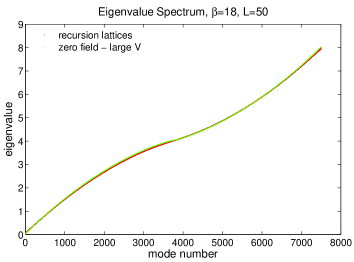
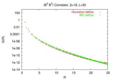
Figure 1: Simulations of the vacuum state at $\beta=18$ and lattice extension $L=50$. (a) Eigenvalue spectra of the operator $-D^{2}-\lambda_{0}+m^{2}$. Also plotted is the spectrum of the large-volume zero-field operator $-\nabla^{2}+m^{2}$. (b) The correlator $G(R)$ computed on recursion and MC lattices.

Fig. 1 is a plot of eigenvalue vs. mode number for the operator $-D^{2}-\lambda_{0}+m^{2}$, at $\beta=18$, from ten independent $50\times 50$ recursion lattices (no averaging). Also plotted, but indistinguishable from the other spectra, is the rescaled spectrum of the large-volume zero-field operator $-\nabla^{2}+m^{2}$. It is obvious from this figure that there is very little variance in the spectrum of $-D^{2}-\lambda_{0}$ from one thermalized lattice to the next, moreover, this spectrum is very close to that of a free-field theory. Fig. 1 shows our data for $G(R)$, obtained from ten recursion lattices, and ten MC lattices. Note the tiny values of $G(R)\sim 10^{-12}$ obtained at the larger R values. This requires a near-absence of fluctuation in $K^{-1}$ from one thermalized lattice to the next. Note also that $G(R)$ obtained on MC and recursion lattices agree very closely with one another. The mass gap $M$ is extracted from a two-parameter $(c,M)$ fit of the recursion lattice data to the function

$$G_{fit}(R)=c(1+{\textstyle{\frac{1}{2}}}MR)^{2}{e^{-MR}\over R^{6}}$$ (16)

The best fit to the data for $G(R)$ at $\beta=18$ is shown in Fig. 2. Our final results for the mass gaps at a variety of $\beta$ values are shown in Fig. 2, together with the results for the $0^{+}$ glueball obtained by Meyer and Teper [16], using standard methods. The agreement is clearly very good.

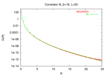
Figure 2: (a) Best fit (dashed line) of the recursion lattice data for $G(R)$ by the analytic form given in eq.  (4.5). (b) Mass gaps extracted from recursion lattices at various lattice couplings, compared to the $0^{+}$ glueball masses in 2+1 dimensions obtained in ref.  [16] (denoted “expt”) via standard lattice Monte Carlo methods. Errorbars are smaller than the symbol sizes.

5 Why confinement?

We have seen that there is a mass gap if $K^{-1}$ has a finite range, and a non-zero string tension (by the dimensional reduction argument) if $K$ is also finite range. Both of these conditions are obtained if the mass parameter $m$ is non-zero, so the question ”why confinement?” boils down to the question: why is $m$ non-zero? An obvious approach is to treat $m$ as a variational parameter, and use it to minimize $\langle H\rangle$ . To simplify matters, noting the negligible fluctuation in $K$, we make the drastic approximations of (i) neglecting functional derivatives of the kernel $K$ in computing $\langle H\rangle$; and (ii) ignoring correlations between $B$ and $K$. With these approximations, the VEV of $H$ turns out to be

$$\langle H\rangle={1\over 2}\left\langle\mbox{Tr}\sqrt{-D^{2}-\lambda_{0}+m^{2}}+{1\over 2}\mbox{Tr}{\lambda_{0}-m^{2}\over\sqrt{-D^{2}-\lambda_{0}+m^{2}}}\right\rangle$$ (17)

There is a competition between the two terms on the rhs; the first increases with $m^{2}$, while the latter decreases. In an abelian theory, where $D^{2}=\nabla^{2}$ and $\lambda_{0}=0$, it is trivial to show that $\langle H\rangle$ is minimized at $m=0$, implying no confinement, and no mass gap in the abelian case. For a non-abelian theory matters are different, chiefly because $\lambda_{0}>0$. A naive calculation, which ignores any dependence of the $\{\lambda_{n}\}$ on $m^{2}$, finds that $m^{2}=\langle\lambda_{0}\rangle$ at the minimum. While a more accurate calculation would no doubt change somewhat the numerical value of $m^{2}$ at the minimum, it seems unlikely that this value would be shifted exactly to zero.

6 What about N-ality?

Dimensional reduction at large scales, from three to two dimensions, implies Casimir scaling of the string tensions; in particular, the adjoint string tension is non-zero. While this is correct at intermediate distance scales, asymptotically the string tension should depend only on the N-ality of the representation. The transition from Casimir scaling to N-ality dependence must be coming from corrections to dimensional reduction.

It is worth examining how N-ality dependence is achieved when the vacuum state is computed by the strong-coupling method developed in ref. [2]. In this case the ground state has the form $\Psi_{0}[U]=\exp[R[U]]$, where $R[U]$ is a sum over contours (plaquette, $1\times 2$ rectangle, etc.) constructed from $p$ plaquettes, with each contour multiplied by a constant of order $\beta^{2p}$. The leading contributions, at strong-coupling, are shown in fig. 3. It is not hard to show that the perimeter law for large adjoint loops is obtained, in the strong-coupling expansion of $\Psi_{0}^{2}[U]$, by tiling the perimeter of the loop with overlapping $1\times 2$ rectangles, as shown in Fig. 3.

Figure 3: (a) The first few terms in the strong-coupling expansion of the lattice vacuum state $\Psi_{0}[U]$, with $R[U]=\log(\Psi_{0}[U])$. (b) How $1\times 2$ rectangles in $R[U]$ screen an adjoint Wilson loop. The adjoint Wilson loop is denoted by a heavy solid line. The overlapping $1\times 2$ rectangles are indicated by (alternately) light solid and light dashed lines.

It is interesting that the rectangle term not only screens adjoint loops, but is also responsible for the leading correction to dimensional reduction. An expansion of the strong-coupling vacuum in powers of lattice spacing yields [17]

$$\Psi_{0}[U]=\exp\left[-{2\over\beta}\int d^{2}x~{}(a\kappa_{0}B^{2}-a^{3}\kappa_{2}B(-D^{2})B+\ldots)\right]$$ (18)

The first term represents dimensional reduction, and all four contours shown in Fig. 3 contribute to $\kappa_{0}$. Only the rectangle contour, however, contributes to the second term, which supplies the leading correction to dimensional reduction. It is also the rectangle contour which couples together field strengths in neighboring plaquettes.

Returning to our proposed vacuum state and expanding the kernel in powers of $1/m^{2}$, the part of $\Psi_{0}^{2}$ quadratic in $B^{slow}$, up to next-to-leading order in $1/m^{2}$, is

$$\exp\left[-{1\over m}\int d^{2}x~{}\left(B^{slow}B^{slow}-B^{slow}{-D^{2}-\lambda_{0}\over 2m^{2}}B^{slow}+\ldots\right)\right]$$ (19)

Note that the correction to the first (dimensional reduction) term is similar to, and has the same sign as, the leading correction to dimensional reduction in the strong-coupling vacuum state, generated by the rectangle term. Our speculation is that, as in strong coupling, this second term is associated with the screening of higher-representation color charges, converting Casimir scaling to N-ality dependence of the higher-representation string tensions.

References

- [1] J. Greensite, Nucl. Phys. B 158, 469 (1979).
- [2] J. Greensite, Nucl. Phys. B 166, 113 (1980).
- [3] M. B. Halpern, Phys. Rev. D19, 517 (1979).
- [4] R. P. Feynman, Nucl. Phys. B 188, 479 (1981).
- [5] P. Mansfield, Nucl. Phys. B418, 113 (1994).
- [6] I. I. Kogan and A. Kovner, Phys. Rev. D 52, 3719 (1995) [arXiv:hep-th/9408081].
- [7] S. Samuel, Phys. Rev. D 55, 4189 (1997) [arXiv:hep-ph/9604405].
- [8] A. P. Szczepaniak and E. S. Swanson, Phys. Rev. D 65, 025012 (2001) [arXiv:hep-ph/0107078].
-
[9]
H. Reinhardt and C. Feuchter,
Phys. Rev. D 71, 105002 (2005)
[arXiv:hep-th/0408237];
H. Reinhardt, D. Epple and W. Schleifenbaum, AIP Conf. Proc. 892, 93 (2007) [arXiv:hep-th/0610324]. - [10] P. Orland, Phys. Rev. D 74, 085001 (2006) [arXiv:hep-th/0607013].
- [11] D. Karabali, C. Kim and V. P. Nair, Phys. Lett. B 434, 103 (1998) [arXiv:hep-th/9804132].
-
[12]
R. G. Leigh, D. Minic and A. Yelnikov, Phys. Rev. Lett. 96,
222001 (2006) [arXiv:hep-th/0512111];
R. G. Leigh, D. Minic and A. Yelnikov, arXiv:hep-th/0604060. - [13] J. M. Cornwall, Phys. Rev. D 76, 025012 (2007) [arXiv:hep-th/0702054].
- [14] D. Diakonov, private communication.
- [15] J. Greensite and Š. Olejník, arXiv:0707.2860 [hep-lat].
- [16] H. Meyer and M. Teper, Nucl. Phys. B 668, 111 (2003) [arXiv:hep-lat/0306019].
- [17] S. H. Guo, Q. Z. Chen and L. Li, Phys. Rev. D 49, 507 (1994).