Sub-luminal wave bullets:  Exact Localized subluminal Solutions to the Wave Equations${}^{\>({\dagger})}$

Michel Zamboni-Rached,

Universidade Federal do ABC, Centro de Sciencias Naturais e Humanas, Santo André, SP;

and DMO–FEEC, State University at Campinas, Campinas, SP, Brazil.

and

Erasmo Recami

Facoltà di Ingegneria, Università statale di Bergamo, Bergamo, Italy;

and INFN—Sezione di Milano, Milan, Italy.

Abstract  –  In this work it is shown how to obtain, in a simple way, localized (non-diffractive) subluminal pulses as exact analytic solutions to the wave equations. These new ideal subluminal solutions, which propagate without distortion in any homogeneous linear media, are herein obtained for arbitrarily chosen frequencies and bandwidths, avoiding in particular any recourse to the non-causal components so frequently plaguing the previously known localized waves. The new solutions are suitable superpositions of —zeroth-order, in general— Bessel beams, which can be performed either by integrating with respect to (w.r.t.) the angular frequency $\omega$, or by integrating w.r.t. the longitudinal wavenumber $k_{z}$: Both methods are expounded in this paper.  The first one appears to be powerful enough;  we study the second method as well, however, since it allows dealing even with the limiting case of zero-speed solutions (and furnishes a new way, in terms of continuous spectra, for obtaining the so-called “Frozen Waves”, so promising also from the point of view of applications).   We briefly treat the case, moreover, of non axially-symmetric solutions, in terms of higher order Bessel beams.  At last, particular attention is paid to the role of Special Relativity, and to the fact that the localized waves are expected to be transformed one into the other by suitable Lorentz Transformations.  The analogous pulses with intrinsic finite energy, or merely truncated, will be constructed in another paper.  In this work we fix our attention especially on electromagnetism and optics: but results of the present kind are valid whenever an essential role is played by a wave-equation (like in acoustics, seismology, geophysics, gravitation, elementary particle physics, etc.).

PACS nos.: 03.50.De;  03.30.+p;  03.50.+p;  41.20.Jb;   41.85.Ct;  42.25.-p;  42.25.Fx;  43.20.+g;  43.20.Ks;  46.40.-f;  46.40.Cd;  47.35.Rs;  52.35.Lv

Keywords: Electromagnetic subluminal bullets; Acoustic subsonic bullets; Optical subluminal bullets; Localized waves; Subluminal pulses; Frozen Waves; Special Relativity; Lorentz transformations; Wave equations; Wave propagation; Bessel beams; Optics; Microwaves; Acoustics; Seismology; Elementary particle wavepackets; Gravitational waves; Mechanical waves.

1 Introduction

Since more than ten years, the so-called (non-diffracting) “Localized Waves” (LW), which are new solutions to the wave equations (scalar, vectorial, spinorial,…), are in fashion, both in theory and in experiment. In particular, rather well-known are the ones with luminal or superluminal peak-velocity: Like the so-called X-shaped waves (see[22, 38] and refs. therein; for a review, see, e.g., ref.[43]), which are supersonic in Acoustics[24], and superluminal in Electromagnetism (see[23] and refs. therein).

Since Bateman[20] and later on Courant & Hilbert[19], it was already known that luminal LWs exist, which are as well solutions to the wave equations. More recently, some attention[3, 63, 30, 14, 15] started to be paid to subluminal solutions too. Let us recall that all the LWs propagate without distortion —and in a self-reconstructive way[55, 2, 59]— in a homogeneous linear medium (apart from local variations).

Like in the superluminal case, the (more orthodox, in a sense) subluminal LWs can be obtained by suitable superpositions of Bessel beams. They have been till now almost neglected, however, for the mathematical difficulties met in getting analytic expressions for them, difficulties associated with the fact that the superposition integral runs over a finite interval.  We want here to re-address the question of such subluminal LWs, showing, by contrast, that one can indeed arrive at exact (analytic) solutions, both in the case of integration over the Bessel beams’ angular frequency $\omega$, and in the case of integration over their longitudinal wavenumber $k_{z}$. The first approach, herein investigated in detail, is enough to get the majority of the desired results; we study also the second one, however, since it allows treating the limiting case of zero-speed solutions (and furnishes a new method —based on a continuous spectrum— for obtaining the so-called “Frozen Waves”, so promising also from the point of view of applications). Moreover, we shall deal with non axially-symmetric solutions, in terms of higher order Bessel beams.  At last, particular attention is paid to the role of Special Relativity, and to the fact that the localized waves are transformed one into the other by Lorentz Transformations.

The present article is devoted to the exact, analytic solutions: i.e., to ideal solutions.  In another paper, we shall go on to the corresponding pulses with finite energy, or truncated, sometimes having recourse —for simplicity, and only in such more realistic cases— to approximations.  We shall fix our attention especially on electromagnetism and optics: but our results are valid whenever an essential role is played by a wave-equation (like in acoustics, seismology, geophysics, gravitation, elementary particle physics, etc.).

Let us recall that, in the past, too much attention had not been paid even to 1983 Brittingham’s paper[41], where he claimed the possibility of obtaining pulse-type solutions to the Maxwell equations, which propagate in free space as a new kind of speed-c “solitons”. This was partially due to the fact that that author was unable to get correct finite-energy expressions for such wavelets, and to make suggestions about their practical production. Two years later, however, Sezginer[42] was able to show how to obtain quasi-nondiffracting luminal pulses endowed with a finite energy. Finite-energy pulses do no longer travel undistorted for an infinite distance, but they can nevertheless propagate without deformation for a long field-depth, much larger than the one achieved by ordinary pulses, as the gaussian ones: Cf., e.g., refs.[36, 37, 18, 13, 5, 9] and refs. therein.

Only after 1985 the general theory of all LWs started to be extensively developed[31, 32, 33, 22, 12, 23, 38, 34, 47, 46] both in the case of beams, and in the case of pulses. For reviews, see for instance the refs.[43, 44, 5, 18, 9] and references therein.  For the propagation of LWs in bounded regions (like guides), see refs.[52, 51, 53, 56] and refs therein.  For the focusing of LWs, see refs.[54, 8] and refs therein. As to the construction of LWs propagating in dispersive media, cf. refs.[25, 48, 49, 57, 17, 7, 50, 45, 6]; and, for lossy media, see ref.[59] and refs. therein.  Al last, for finite-energy, or truncated, solutions see refs.[35, 9, 38, 51, 39, 61].

By now, the LWs have been experimentally produced[24, 26, 27], and are being applied in fields ranging from ultrasound scanning[28, 29, 30] to optics (for the production, e.g., of new type of tweezers[62]). All these works demonstrated that nondiffracting pulses can travel with an arbitrary peak-speed $v$, that is, with $0<v<\infty$; while Brittingham e Sezginer had confined themselves to the luminal case ($v=c$) only. As already commented, the superluminal and luminal LWs have been, and are being, intensively studied, whilst the subluminal ones have been neglected: Almost all the few papers dealing with them had till now recourse to the paraxial[58] approximation[11], or to numerical simulations[14], due to the above mentioned mathematical difficulty in obtaining exact analytic expressions for subluminal pulses. Actually, only one analytic solution is known[3, 12, 63, 30, 11] biased by the physically unconvenient facts that its frequency spectrum is very large, it doesn’t even possess a well-defined central frequency, and, even more, that non-causal (i.e., backwards traveling)[32, 9] components are a priori needed for constructing it.  Aim of the present paper is showing how subluminal localized exact solutions can be constructed with any spectra, in any frequency bands and for any bandwidths; and, moreover, without employing[38, 5] any non-causal components.

2 A first method for constructing physically
acceptable, subluminal Localized Pulses

Axially symmetric solutions to the scalar wave equation are known to be superpositions of zero-order Bessel beams over the angular frequency $\omega$ and the longitudinal wavenumber $k_{z}$: i.e., in cylindrical co-ordinates,

$$\Psi(\rho,z,t)\;=\;\int_{0}^{\infty}\,{\rm d}\omega\,\int_{-\omega/c}^{\omega/c}\,{\rm d}k_{z}\,\overline{S}(\omega,k_{z})J_{0}\left(\rho\sqrt{\frac{\omega^{2}}{c^{2}}-k_{z}^{2}}\right)e^{ik_{z}z}e^{-i\omega t}\;,$$ (1)

where  $k_{\rho}^{2}\equiv\omega^{2}/c^{2}-k_{z}^{2}$  is the transverse wavenumber; quantity $k_{\rho}^{2}$ has to be positive if one does not want to deal with evanescent waves.

The condition characterizing a nondiffracting wave is the existence[9, 10] of a linear relation between longitudinal wavenumber $k_{z}$ and frequency $\omega$ for all the Bessel beams entering superposition (1); that is to say, the chosen spectrum has to entail[38, 18] for each Bessel beam a linear relationship of the type  (cf. Fig.1):

$$\omega\;=\;v\,k_{z}+b\;\,$$ (2)

with $b\geq 0$.  Requirement (2) can be regarded also as a specific space-time coupling, implied by the chosen spectrum $\overline{S}$. Equation (2) has to be obeyed by the spectra of any one of the three possible types (subluminal, luminal or superluminal) of nondiffracting pulses.  Let us mention, incidentally, that with the choice in Eq.(2) the pulse re-gains its initial shape after the space-interval ${\Delta z}_{1}=2\pi v/b$;  the more general case can be, however, considered[38, 6] when $b$ assumes any values $b_{m}=m\,b$ (with $m$ an integer), and the periodicity space-interval becomes ${\Delta z}_{m}={\Delta z}_{1}/m\,$.

In the subluminal case, of interest here, the only exact solution known till now, represented by Eq.(10) below, is the one found by Mackinnon[3]. Indeed, by taking into explicit account that the transverse wavenumber $k_{\rho}$ of each Bessel beam entering Eq.(1) has to be real, it can be easily shown (as first noticed by Salo et al. for the analogous acoustic solutions[14]) that in the subluminal case $b$ cannot vanish, but must be larger than zero:  $b>0$.  Then, by using conditions (2) and $b>0$, the subluminal localized pulses can be expressed as integrals over the frequency only:

$$\Psi(\rho,z,t)\;=\;\exp{[-ib{z\over v}]}\,\int_{\omega_{-}}^{\omega_{+}}\,{\rm d}\omega\;S(\omega)\,J_{0}(\rho k_{\rho})\,\exp{[i\omega{\zeta\over v}]}\;,$$ (3)

where now

$$k_{\rho}\;=\;{1\over v}\,\sqrt{2b\omega-b^{2}-(1-v^{2}/c^{2})\omega^{2}}\;\,$$ (4)

with

$$\zeta\,\equiv\,z-vt\;\,$$ (5)

and with

$\left\{\begin{array}[]{clr}\omega_{-}\;=\;\displaystyle{{b\over{1+v/c}}}\\ \\ \omega_{+}\;=\;\displaystyle{{b\over{1-v/c}}}\end{array}\right.$ (6)

As anticipated, the Bessel beam superposition in the subluminal case results to be an integration over a finite interval of $\omega$, which, by the way, does clearly shows that the non-causal (backwards traveling) components correspond to the interval $\omega_{-}<\omega<b$.  It could be noticed, incidentally, that Eq.(3) does not represent the most general exact solution, which on the contrary is a sum[6] of such solutions for the various possible values of $b$ just mentioned above: That is, for the values $b_{m}=m\,b$ and spatial periodicity ${\Delta z}_{m}={\Delta z}_{1}/m\,$; but we can confine ourselves to solution (3) without any real loss of generality, since the actual problem is evaluating in analytic form the integral entering Eq.(3). For any mathematical and physical details, see ref.[6].

Now, if one adopts the change of variables

$$\omega\,\equiv\,{b\over{1-v^{2}/c^{2}}}\;(1+{v\over c}s)\;\,$$ (7)

equation (3) becomes[14]

$$\Psi(\rho,z,t)\;=\;{b\over c}\,{v\over{1-v^{2}/c^{2}}}\,\exp{[-i{b\over v}z]}\;\exp{\left[i{b\over v}\,{1\over{1-v^{2}/c^{2}}}\,\zeta\right]}$$ (8)

$${}\times\int_{-1}^{1}\,{\rm d}s\;S(s)\,J_{0}\left({b\over c}\,{\rho\over{\sqrt{1-v^{2}/c^{2}}}}{\sqrt{1-s^{2}}}\right)\;\exp{\left[i{b\over c}{1\over{1-v^{2}/c^{2}}}\zeta s\right]}\;.$$

In the following we shall adhere to some symbols standard in Special Relativity (since the whole topic of subluminal, luminal and superluminal LWs is strictly connected[43, 23, 21] with the principles and structure of special relativity [cf.[1, 16] and refs. therein], as we shall mention in the Conclusions); namely:

$$\beta\equiv{v\over c}\;;\ \ \ \ \ \ \ \ \ \gamma\,\equiv\,{1\over{\sqrt{1-\beta^{2}}}}\;.$$ (9)

As already said, Eq.(8) has till now yielded one analytic solution for $S(s)\,=\;$constant, only (for instance, $S(s)=1$); which means nothing but $S(\omega)\,=\;$constant: in this case one gets indeed the Mackinnon solution[3, 12, 30, 61]

$$\Psi(\rho,\zeta,\eta)\;=\;2{b\over c}v\,\gamma^{2}\,{\exp{\left[i{b\over c}\,\beta\gamma^{2}\;\eta\right]}}$$ (10)

$${}\times{\rm sinc}\ {\sqrt{{b^{2}\over c^{2}}\,\gamma^{2}\left(\rho^{2}+\gamma^{2}\;\zeta^{2}\right)}}\;,$$

which however, for its above-mentioned drawbacks, is endowed with little physical and practical interest.  In Eq.(9) the ${\rm sinc}$ function is defined as

$${\rm sinc}\ x\,\equiv\,(\sin\;x)/x\;,$$

and

$$\eta\,\equiv\,z-Vt,\ \ \ \ \ \ \ {\rm with}\ \ V\equiv{c^{2}\over v}\;,$$ (11)

where $V$ and $v$ are related by the de Broglie relation.  [Notice that $\Psi$ in Eq.(10), and in the following ones, is eventually a function (besides of $\rho$) of $z,t$ via $\zeta$ and $\eta$, both functions of $z$ and $t\;$].

We can, however, construct by a very simple method new subluminal pulses corresponding to whatever spectrum, and devoid of non-causal (entering) components, by taking also advantage of the fact that in our equation (8) the integration interval is finite: that it, by transforming it in a good, instead of a harm. Let us first observe that Eq.(10) doesn’t admit only the already known analytic solution corresponding to $S=constant$, and more in general to $S(\omega)\,=\;$constant, but it will also yield an exact, analytic solution for any exponential spectra of the type

$$S(\omega)\;=\;\exp{[{i2n\pi\omega\over\Omega}]}\;,$$ (12)

with $n$ any integer number, which means for any spectra of the type $S(s)=\exp{[in\pi/\beta]}\,\exp{[in\pi s]}$, as can be easily seen by checking the product of the various exponentials entering the integrand.  In Eq.(12) we have set

$$\Omega\,\equiv\,{\omega_{+}}-{\omega_{-}}\;.$$

The solution writes in this more general case:

$$\Psi(\rho,\zeta,\eta)\;=\;2b\beta\,\gamma^{2}\,\exp{\left[i{b\over c}\,\beta\,\gamma^{2}\,\eta\right]}$$ (13)

$${}\times\exp{[in{\pi\over\beta}]}\ {\rm sinc}\ {\sqrt{{b^{2}\over c^{2}}\,\gamma^{2}\,\rho^{2}+\left({b\over c}\,\gamma^{2}\,\zeta+n\pi\right)^{2}}}\;.$$

Let us explicitly notice that also in Eq.(13) quantity $\eta$ is defined as in Eqs.(11) above, where $V$ and $v$ obey the de Broglie relation $vV=c^{2}$, the subluminal quantity $v$ being the velocity of the pulse envelope, and $V$ playing the role (in the envelope’s interior) of a superluminal phase velocity.

The next step, as anticipated, consists just in taking advantage of the finiteness of the integration limits for expanding any arbitrary spectra $S(\omega)$ in a Fourier series in the interval $\omega_{-}\leq\omega\leq\omega_{+}\;$:

$$S(\omega)\;=\;\sum_{n=-\infty}^{\infty}\,A_{n}\,\exp{[+in{2\pi\over\Omega}\omega]}\;,$$ (14)

where (we can go back, now, from the $s$ to the $\omega$ variable):

$$A_{n}\;=\;{1\over\Omega}\,\int_{\omega_{-}}^{\omega_{+}}{\rm d}\omega\,S(\omega)\,\exp{[-in{2\pi\over\Omega}\omega]}\;\,$$ (15)

quantity $\Omega$ being defined as above.

Then, on remembering the special solution (13), we can infer from expansion (14) that, for any arbitrary spectral function $S(\omega)$, a rather general, axially-symmetric, analytic solution for the subluminal case can be written

$$\Psi(\rho,\zeta,\eta)\;=\;2b\beta\,\gamma^{2}\,{\exp{\left[i{b\over c}\,\beta\,\gamma^{2}\;\eta\right]}}$$ (16)

$${}\times\sum_{n=-\infty}^{\infty}\,A_{n}\,\exp{[in{\pi\over\beta}]}\ {\rm sinc}\ {\sqrt{{b^{2}\over c^{2}}\,\gamma^{2}\rho^{2}+\left({b\over c}\gamma^{2}\;\zeta+n\pi\right)^{2}}}\;,$$

in which the coefficients $A_{n}$ are still given by Eq.(15). Let us repeat that our solution is expressed in terms of the particular equation (13), which is a Mackinnon-type solution.

The present approach presents many advantages. We can easily choose spectra localized within the prefixed frequency interval (optical waves, microwaves, etc.) and endowed with the desired bandwidth. Moreover, as already said, spectra can now be chosen such that they have zero value in the region $\omega_{-}\leq\omega\leq b$, which is responsible for the non-causal components of the subluminal pulse.

Let us stress that, even when the adopted spectrum $S(\omega)$ does not possess a known Fourier series (so that the coefficients $A_{n}$ cannot be exactly evaluated via Eq.(15)), one can calculate approximately such coefficients without meeting any problem, since our general solutions (8) will still be exact solutions.

Let us set forth in the following some examples.

2.1 Some Examples

In general, optical pulses generated in the lab possess a spectrum centered on some frequency value, $\omega_{0}$, called the carrier frequency.  The pulses can be, for instance, ultra short, when $\Delta\omega/\omega_{0}\geq 1$; or quasi monochromatic, when $\Delta\omega/\omega_{0}<<1$, where $\Delta\omega$ is the spectrum bandwidth.

These kinds of spectra can be mathematically represented by a gaussian function, or functions with similar behavior.

First Example:

Let us consider a gaussian spectrum

$$S(\omega)\;=\;\frac{a}{\sqrt{\pi}}\exp{[-a^{2}(\omega-\omega_{0})^{2}]}$$ (17)

whose values are negligible outside the frequency interval $\omega_{-}<\omega<\omega_{+}$ over which the Bessel beams superposition in Eq.(3) is made, it being $\omega_{-}=b/(1+\beta)$ and $\omega_{+}=b/(1-\beta)$.  Of course, relation (2) has still to be satisfied, and with $b>0$, for getting an ideal subluminal localized solution.  Notice that, with spectrum (17), the bandwidth (actually, the FWHM) results to be $\Delta\omega=2/a$.  Let us emphasize that, once $v$ and $b$ have been fixed, the values of $a$ and $\omega_{0}$ can then be selected in order to kill the backwards-traveling components, that exist, as we know (cf. Fig.1) for $\omega<b\;$.

The Fourier expansion in Eq.(14), which yields, with the above spectral function (17), the coefficients

$$A_{n}\,\simeq\,\displaystyle{{{1}\over{W}}}\,\exp{[-in{2\pi\over\Omega}\omega_{0}]}\;\exp{[{{-n^{2}\pi^{2}}\over{a^{2}W^{2}}}]}\;,$$ (18)

constitutes an excellent representation of the gaussian spectrum (17) in the interval $\omega_{-}<\omega<\omega_{+}$ (provided that, as we requested, our gaussian spectrum does get negligible values outside the frequency interval $\omega_{-}<\omega<\omega_{+}$).

In other words, on choosing a pulse velocity $v<c$ and a value for the parameter $b$, a subluminal pulse with the above frequency spectrum (17) can be written as Eq.(15), with the coefficients $A_{n}$ given by Eq.(18): The evaluation of such coefficients $A_{n}$ being rather simple.  Let us repeat that, even if the values of the $A_{n}$ are obtained via a (rather good, by the way) approximation, we based ourselves on the exact solution Eq.(16).

One can, for instance, obtain exact solutions representing subluminal pulses for optical frequencies. Let us get the subluminal pulse with velocity $v=0.99\;c$, angular carrier frequency $\omega_{0}=2.4\times 10^{15}\;$Hz (that is, $\lambda_{0}=0.785\;\mu$m) and bandwidth (FWHM) $\Delta\omega=\omega_{0}/20=1.2\times 10^{14}\;$Hz, which is an optical pulse of $24$ fs (that is the FWHM of the pulse intensity).  For a complete pulse characterization, one has to choose the value of the frequency $b$: let it be $b=3\times 10^{13}\;$Hz; as a consequence one has $\omega_{-}=1.507\times 10^{13}\;$Hz and $\omega_{+}=3\times 10^{15}\;$Hz.  [This is exactly a case in which the considered pulse is not plagued by the presence of non-causal components, since the chosen spectrum forwards totally negligible values for $\omega<b$].  The construction of the pulse does already result satisfactory when considering about 51 terms ($-25\leq n\leq 25$) in the series entering Eq.(16).

Figures 2 show our pulse, plotted by considering the mentioned fifty-one terms. Namely: Fig.(a) depicts the orthogonal projection of the pulse intensity;  Fig.(b) shows the three-dimensional intensity pattern of the real part of the pulse, which reveals the carrier wave oscillations.

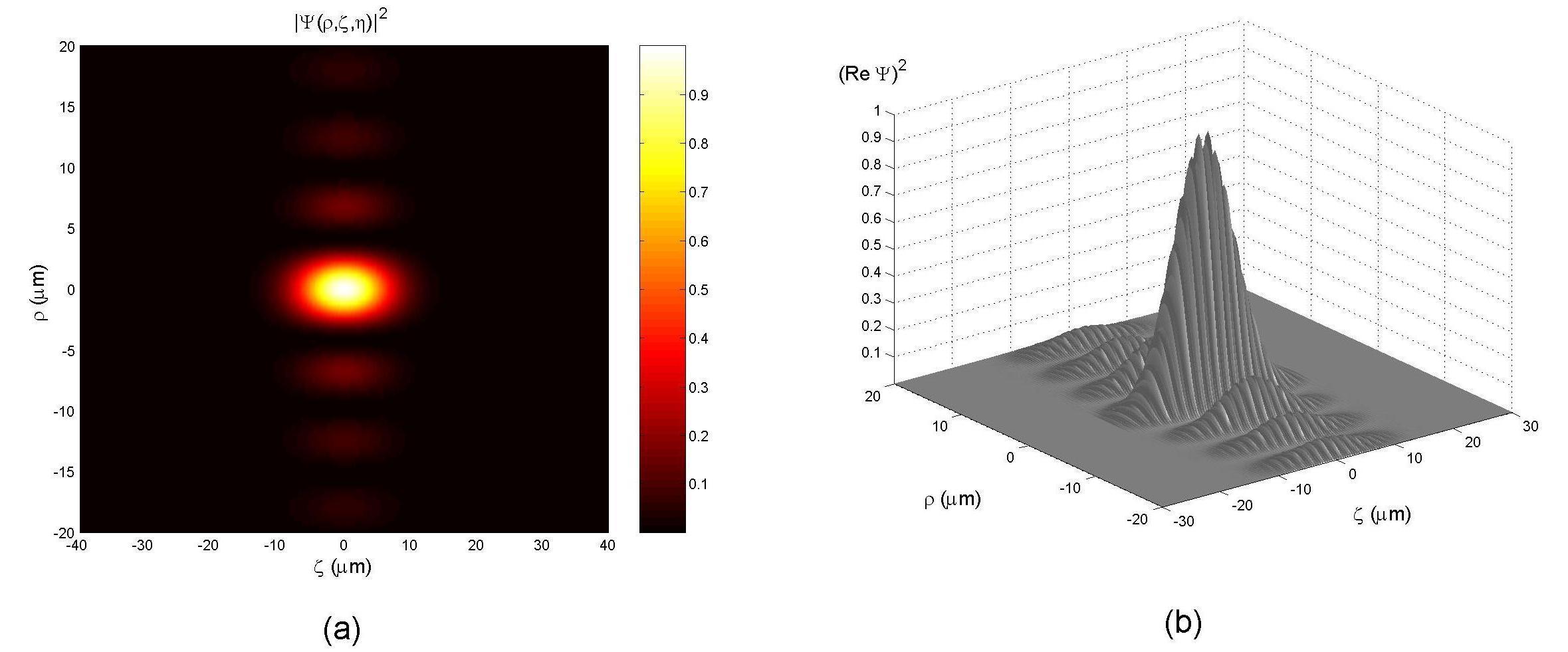
Figure 1: (a) The orthogonal projection of the pulse intensity;  (b) The three-dimensional intensity pattern of the real part of the pulse, which reveals the carrier wave oscillations.

Let us stress that the ball-like shape for the field intensity should be typically associated with all the subluminal LWs, while the typical superluminal ones are known to be X-shaped[22, 23, 21], as predicted, since long, by special relativity in its “non-restricted” version: See refs.[1, 16, 23, 43] and refs therein.

Another interesting spectrum $S(\omega)$ would be, for example, the “inverted parabola” one, centered at the frequency $\omega_{0}$: that is,

$$S(\omega)\;=\;\left\{\begin{array}[]{clr}{\frac{-4\,[\omega-(\omega_{0}-\Delta\omega/2)][\omega-(\omega_{0}+\Delta\omega/2)]}{\Delta\omega^{2}}}&{\rm for}\;\;\;\omega_{0}-\Delta\omega/2\leq\omega\leq\omega_{0}+\Delta\omega/2\\ \\ \;\;\;\;\;\;0&{\rm otherwise}\ ,\end{array}\right.$$ (19)

where $\Delta\omega$, the distance between the two zeros of the parabola, can be regarded as the spectrum bandwidth.  One can expand $S(\omega)$, given in Eq.(19), in the Fourier series (14), for $\omega_{-}\leq\omega\leq\omega_{+}\;$, with coefficients $A_{n}$ that —even if straightforwardly calculable— results to be complicated, so that we skip reporting them here explicitly.  Let us here only mention that spectrum (19) may be easily used to get, for instance, an ultrashort (femtasecond) optical non-diffracting pulse, with satisfactory results even when considering very few terms in expansion (14).

Second Example:

As a second example, let us consider the very simple case when —within the integration limits $\omega_{-}$, $\omega_{+}$— the complex exponential spectrum (12) is replaced by the real function (still linear in $\omega$)

$$S(\omega)\;=\;\frac{a}{1-\exp{[-a(\omega_{+}-\omega_{-})]}}\,\exp{[a(\omega-\omega_{+}]}\;,$$ (20)

with $a$ a positive number [for $a=0$ one goes back to the Mackinnon case]. Spectrum (20) is exponentially concentrated in the proximity of $\omega_{+}$, where it reaches its maximum value; and becomes more and more concentrated (on the left of $\omega_{+}$, of course) as the arbitrarily chosen value of $a$ increases, with the frequency bandwidth being $\Delta\omega=1/a$. Let us recall, incidentally, that, on its turn, quantity $\omega_{+}$ and $\omega_{-}$ depend on the pulse velocity $v$ and on the arbitrary parameter $b$.

By performing the integration as in the case of spectrum (12), instead of solution (13) in the present case one eventually gets the solution

$$\Psi(\rho,\zeta,\eta)\;=\;\frac{2ab\beta\gamma^{2}\,\exp{[ab\gamma^{2}]}\,\exp{[-a\omega_{+}]}}{1-\exp{[-a(\omega_{+}-\omega_{-})]}}$$ (21)

$${}\times\exp{\left[i{b\over c}\,\beta\,\gamma^{2}\,\eta\right]}\ {\rm sinc}{\left[{b\over c}\,\gamma^{2}\;{\sqrt{\gamma^{-2}\,\rho^{2}-(av+i\zeta)^{2}}}\right]}\;.$$

After Mckinnon’s, this eq.(21) appears to be the simplest closed-form solution, since both of them do not need any recourse to series expansions. In a sense, our solution (21) might be regarded as the subluminal analogous of the (superluminal) X-wave solution; a difference being that the standard X-shaped solution has a spectrum starting with 0, where it assumes its maximum value, while in the present case the spectrum starts at $\omega_{-}$ and gets increasing afterwards till $\omega_{+}$ . More important is to observe that the gaussian spectrum has a priori two advantages w.r.t. eq.(20): It may be more easily centered around any value $\omega_{0}$ of $\omega$, and, when increasing its concentration in the surrounding of $\omega_{0}$, the spot transverse width does not increase indefinitely, but tends to the spot width of a Bessel beam with $\omega=\omega_{0}$ and $k_{z}=(\omega_{0}-b)/V$, at variance with what happens for spectrum (20); however, solution (21) is noticeable, since it is really the simplest one.

Figure 3 show the intensity of the real part of the subluminal pulse corresponding to this spectrum, with $v=0.99\;c$, $b=3\times 10^{13}\;$Hz (which result in $\omega_{-}=1.5\times 10^{13}\;$Hz and $\omega_{-}=3\times 10^{15}\;$Hz), $\Delta\omega/\omega_{+}=1/100$ (i.e., $a=100$). This is an optical pulse of $0.2$ ps.

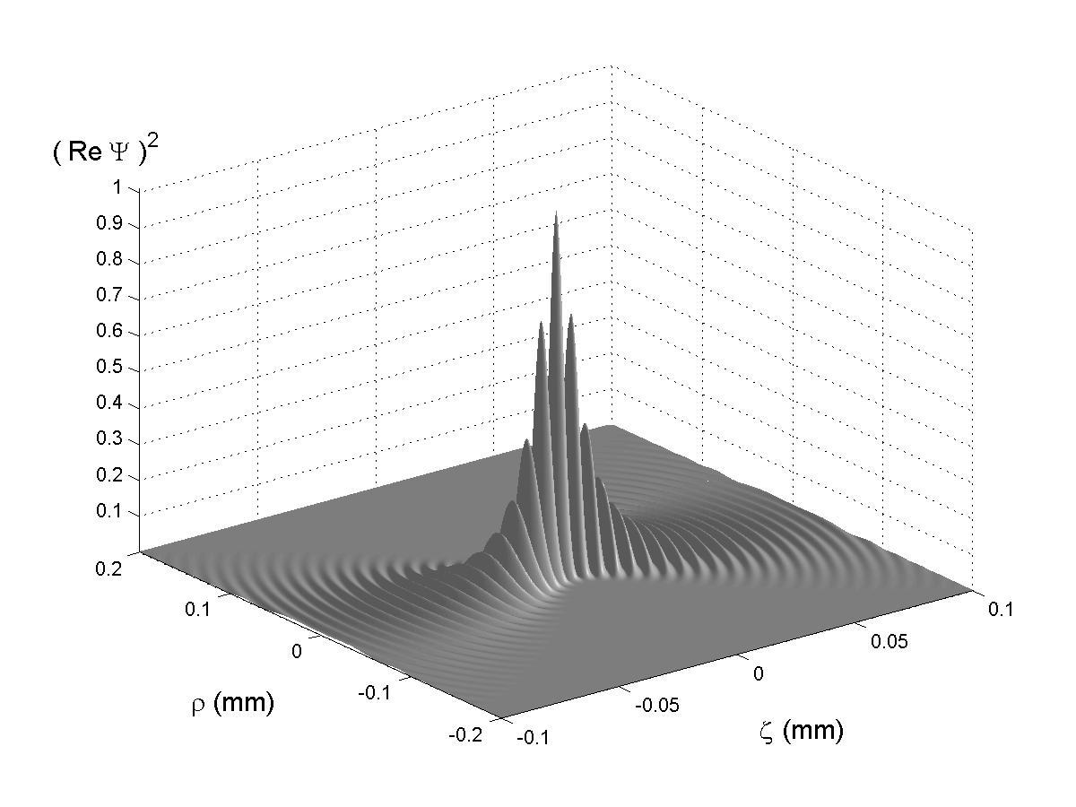
Figure 2: The intensity of the real part of the subluminal pulse corresponding to spectrum (20), with $v=0.99\;c$, $b=3\times 10^{13}\,$Hz (which result in $\omega_{-}=1.5\times 10^{13}\;$Hz and $\omega_{-}=3\times 10^{15}\;$Hz), $\Delta\omega/\omega_{+}=1/100$ (i.e., $a=100$).

3 A second method for constructing
subluminal Localized Pulses

The previous method appears to be very efficient for finding out analytic subluminal LWs, but it looses its validity in the limiting case $v\rightarrow 0$, since for $v=0$ it is $\omega_{-}\equiv\omega_{+}$ and the integral in Eq.(3) degenerates, furnishing a null value.  By contrast, we are interested also in the $v=0$ case, since it corresponds to some of the most interesting, and potentially useful, LWs: Namely, to the so-called “Frozen Waves”, which are new stationary solutions to the wave equations, possessing a static envelope.

It is possible to solve this problem by starting again from Eq.(1), with constraint (2), but going on —this time— to integrals over $k_{z}$. instead of over $\omega$.  It is enough to write relation (2) in the form

$k_{z}\;=\;\displaystyle{{1\over v}\,(\omega-b)}$ (2’)

for expressing the exact solutions (1) as

$$\Psi(\rho,z,t)\;=\;\exp{[-ibt]}\;\int_{k_{z}{\rm min}}^{k_{z}{\rm max}}\,{\rm d}k_{z}\;S(k_{z})\,J_{0}(\rho k_{\rho})\,\exp{[i\zeta k_{z}]}\;,$$ (22)

with

$\left\{\begin{array}[]{clr}k_{z}{\rm min}\;=\;\displaystyle{{-b\over c}\,{1\over{1+\beta}}}\\ \\ k_{z}{\rm max}\;=\;\displaystyle{{b\over c}\,{1\over{1-\beta}}}\end{array}\right.$ (23)

and with

$${k_{\rho}}^{2}\;=\;-{k_{z}^{2}\over\gamma^{2}}+2{b\over c}\beta k_{z}+{b^{2}\over c^{2}}\;,$$ (24)

where quantity $\zeta$ is still defined according to Eq.(5), always with $v<c$.

One can show that the unique exact solution previously known[3] may be rewritten in the form of Eq.(24) with $S(k_{z})=\;$constant.  Then, on following the same procedure exploited in our first method (previous Section), one can find out new exact solutions corresponding to

$$S(k_{z})\;=\;\exp{[{i2n\pi k_{z}\over K}]}\;,$$ (25)

where

$$K\,\equiv\,k_{z}{\rm max}-{k_{z}{\rm min}}\;,$$

by performing the change of variable [analogous, in its finality, to the one in Eq.(7)]

$$k_{z}\,\equiv\,{b\over c}\,\gamma^{2}\,(s+\beta)\;.$$ (26)

At the end, the exact subluminal solution corresponding to the spectrum (25) results to be

$$\Psi(\rho,\zeta,\eta)\;=\;2\,{b\over c}\,\gamma^{2}\,\exp{[i{b\over c}\,\beta\,\gamma^{2}\,\eta]}$$ (27)

$${}\times\exp{[in\pi\beta]}\ {\rm sinc}\ {\sqrt{{b^{2}\over c^{2}}\,\gamma^{2}\,\rho^{2}+\left({b\over c}\,\gamma^{2}\,\zeta+n\pi\right)^{2}}}\;,$$

We can again observe that any spectra $S(k_{z})$ can be expanded, in the interval $k_{z}{\rm min}<k_{z}<k_{z}{\rm max}$, in a Fourier series:

$$S(k_{z})\;=\;\sum_{n=-\infty}^{\infty}\,A_{n}\,\exp{[+in{2\pi\over K}k_{z}]}\;,$$ (28)

with coefficients given now by

$$A_{n}\;=\;{1\over K}\,\int_{k_{z}{\rm min}}^{k_{z}{\rm max}}{\rm d}k_{z}\,S(k_{z})\,\exp{[-in{2\pi\over K}k_{z}]}\;\,$$ (29)

quantity $K$ having been defined above.

At the very end of the whole procedure, the general exact solution representing a subluminal LW, for any spectra $S(k_{z})$, can be eventually written

$$\Psi(\rho,\zeta,\eta)\;=\;2\,{b\over c}\,\gamma^{2}\,\exp{[i{b\over c}\,\beta\,\gamma^{2}\,\eta]}$$ (30)

$${}\times\sum_{n=-\infty}^{\infty}\,A_{n}\,\exp{[in\pi\beta]}\ {\rm sinc}\ {\sqrt{{b^{2}\over c^{2}}\,\gamma^{2}\,\rho^{2}+\left({b\over c}\,\gamma^{2}\,\zeta+n\pi\right)^{2}}}\;,$$

whose coefficients are expressed in Eq.(29), and where quantity $\eta$ is defined as above, in Eq.(11).

Interesting examples could be easily worked out, as we did at the end of the previous Section.

4 Stationary solutions with zero-speed envelopes
(“Frozen Waves”)

Here, we shall refer ourselves to the (second) method, expounded in the previous Section.  Our solution (30), for the case of envelopes at rest, that is, in the case $v=0$ [which implies $\zeta=z$], becomes

$\Psi(\rho,z,t)\;=\;\displaystyle{2\,{b\over c}\;\exp{[-ibt]}\;\sum_{n=-\infty}^{\infty}\,A_{n}\ {\rm sinc}\ {\sqrt{{b^{2}\over c^{2}}\,\rho^{2}+\left({b\over c}\,z+n\pi\right)^{2}}}}\;,$ (31)

with coefficients $A_{n}$ given by Eq.(29) with $v=0$, so that its integration limits simplify into $-b/c$ and $b/c$, respectively; thus, one gets

$A_{n}\;=\;\displaystyle{{c\over{2b}}\,\int_{-b/c}^{b/c}{\rm d}k_{z}\,S(k_{z})\,\exp{[-in{c\pi\over b}k_{z}]}}\;.$ (29’)

Equation (31) is a new, exact solution, corresponding to stationary beams with a static intensity envelope.  Let us observe, however, that even in this case one has energy propagation, as it can be easily verified from the power flux $\mbox{\boldmath$S$}=-\mbox{\boldmath$\nabla$}\Psi\ \partial\Psi/\partial t$ (scalar case) or from the Poynting flux $\mbox{\boldmath$S$}=(\mbox{\boldmath$E$}\wedge\mbox{\boldmath$H$})$ (vectorial case: the condition being that $\Psi$ be a single component, $A_{z}$, of the vector potential $A$).[23]  For $v=0$, eq.(2) becomes

$$\omega\;=\;b\,\equiv\,\omega_{0}\;,$$

so that the particular subluminal waves endowed with null velocity are actually monochromatic beams.

It may be stressed that the present (second) method does yield exact solutions, without any need of the paraxial approximation, which, on the contrary, is so often used when looking for expressions representing beams, like the gaussian ones.  Let us recall that, when having recourse to the paraxial approximation, the obtained beam expressions are valid only when the envelope sizes (e.g., the beam spot) vary in space much more slowly than the beam wavelength. For example, the usual expression for a gaussian beam[58] holds only when the beam spot $\Delta\rho$ is much larger than $\lambda_{0}\equiv\omega_{0}/(2\pi c)=b/(2\pi c)$: so that those beams cannot be very much localized.  By contrast, our method overcomes such problems, since it provides us, as we have seen above, with exact expressions for (well localized) beams with sizes of the order of their wavelength.  Notice, moreover, that the already-known exact solutions —for instance, the Bessel beams— are nothing but particular cases of our solution (31).

An example:  On choosing (with $0\leq q_{-}<q_{+}\leq 1$) the spectral double-step function

$S(k_{z})\;=\;\left\{\begin{array}[]{clr}\displaystyle{\frac{c}{\omega_{0}(q_{+}-q_{-})}}&{\rm for}\ q_{-}\omega_{0}/c\leq k_{z}\leq q_{+}\omega_{0}/c\\ \\ 0&{\rm elsewhere}\;,\end{array}\right.$ (32)

the coefficients of Eq.(31) become

$A_{n}\;=\;\displaystyle{\frac{ic}{2\pi n\omega_{0}(q_{+}-q_{-})}\;\left[e^{-iq_{+}\pi n}-e^{-iq_{-}\pi n}\right]}\;.$ (33)

The double-step spectrum (32), with regard to the longitudinal wave number, corresponds to the mean value $\overline{k}_{z}=\omega_{0}(q_{+}+q_{-})/2c$ and to the width $\Delta k_{z}=\omega_{0}(q_{+}-q_{-})/c$. From these relations, it follows that $\Delta k_{z}/\overline{k}_{z}=2(q_{+}-q_{-})/(q_{+}+q_{-})$.

For values of $q_{-}$ and $q_{+}$ that do not satisfy the inequality $\Delta k_{z}/\overline{k}_{z}<<1$, the resulting solution will be a non-paraxial beam.

Figures 3 show the exact solution corresponding to $\omega_{0}=1.88\times 10^{15}\;$Hz (i.e., $\lambda_{0}=1\;\mu$m) and to $q_{-}=0.3$, $q_{+}=0.9$, which results to be a beam with a spot-size diameter of $0.6\;\mu$m, and, moreover, with a rather good longitudinal localization.  In the case of Eqs.(32,33), about 21 terms ($-10\leq n\leq 10$) in the sum entering Eq.(31) are quite enough for a good evaluation of the series. The beam considered in this example is highly non-paraxial (with $\Delta k_{z}/\overline{k}_{z}=1$ ), and therefore couldn’t have been obtained by ordinary gaussian beam solutions (which are valid in the paraxial regime only).

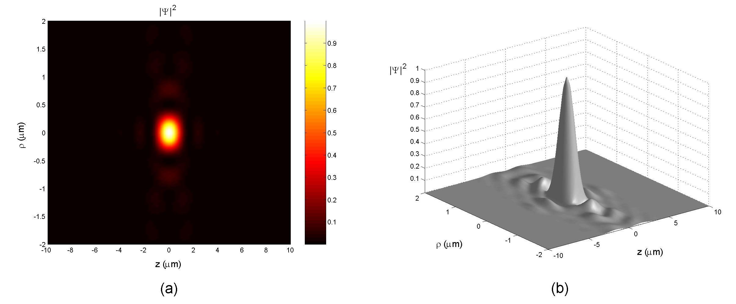
Figure 3: (a) Orthogonal projection of the three-dimensional intensity pattern of the beam (a null-speed subluminal wave) corresponding to spectrum (32);  (b) 3D plot of the field intensity. The beam considered in this example is highly non-paraxial.

Let us now emphasize that a noticeable property of our present method is that it allows a spatial modeling even of monochromatic fields (that correspond to envelopes at rest; so that, in the electromagnetic cases, one can speak, e.g., of the modeling of “light-fields at rest”).  Such a property —rather interesting, especially for applications[62]— was already investigated, under different assumptions, in refs.[39, 40, 59], where the stationary fields with static envelopes were called “Frozen Waves” (FW).  Namely, in the quoted references, discrete superpositions of Bessel beams were adopted in order to get a predetermined longitudinal (on-axis) intensity pattern, inside the desired space interval $0<z<L$.  In other words, in refs.[39, 40, 59], the Frozen Waves have been written in the form

$\begin{array}[]{clr}\Psi(\rho,z,t)\;=\;\displaystyle{e^{-i\omega_{0}t}\ e^{iQz}}\\ \\ \ \ \ \ \ \ \ \ \ \ \times\displaystyle{\sum_{n=-N}^{N}\,B_{n}\;J_{0}(\rho{k_{\rho}}_{n})\;e^{i2n\pi z/c}}\end{array}$ (34)

with

$B_{n}\;=\;\displaystyle{{1\over L}\,\int_{0}^{L}{\rm d}z\;F(z)\ e^{-i2n\pi z/L}}\;,$ (35)

quantity $|F(z)|^{2}$ being the desired longitudinal intensity shape, chosen a priori.  In Eq.(35), it is  ${{k_{\rho}}_{n}}^{2}=n^{2}\omega^{2}/c^{2}-{{k_{z}}_{n}}^{2}$,  and  $0\leq Q+2N\pi/L\leq\omega_{0}/c$,  were we put  ${{k_{z}}_{n}}\equiv Q+2n\pi/n$.  As we see from Eq.(34), the FWs have been represented in the past in terms of discrete superpositions of Bessel beams.  But, now, the method exploited in this paper allows us to go on to dealing with continuous superpositions. In fact, the continuous superposition analogous to eq.(34) would write

$\Psi(\rho,z,t)\;=\;\displaystyle{e^{-i\omega_{0}t}\;\int_{-\omega_{0}/c}^{\omega_{0}/c}{\rm d}k_{z}\ S(k_{z})\ J_{0}(\rho k_{\rho})\ e^{izk_{z}}}\;,$ (36)

which, actually, is nothing but our previous Eq.(22) with $v=0$ (and therefore $\zeta=z$):  That is, eq.(36) does just represent a null-speed subluminal wave.  To be clearer, let us recall that the FWs were expressed in the past as discrete superposition, mainly because it was not known at that time how to treat analytically a continuous superposition like eq.(36). Only by following the method presented in this work one can eventually extend the FW approach[39, 40, 59] to the case of integrals: without numerical simulations, but in terms once more of analytic solutions.

Indeed, the exact solution of Eq.(36) is given by Eq.(31), with coefficients (29’). And one can choose the spectral function $S(k_{z})$ in such a way that $\Psi$ assumes the on-axis pre-chosen static intensity pattern $|F(z)|^{2}$. Namely, the equation to be satisfied by $S(k_{z})$, to such an aim, comes by associating eq.(36) with the requirement $|\Psi(\rho=0,z,t)|^{2}=|F(z)|^{2}$, which entails the integral relation

$\displaystyle{\int_{-\omega_{0}/c}^{\omega_{0}/c}{\rm d}k_{z}\;S(k_{z})\;e^{izk_{z}}}\;=\;F(z)\;.$ (37)

Equation (37) would be trivially soluble in the case of an integration between $-\infty$ and $+\infty$, since it would merely be a Fourier transformation; but obviously this is not the case, because its integration limits are finite. Actually, there are functions $F(z)$ for which Eq.(37) is not soluble, in the sense that no spectra $S(k_{z})$ exist obeying the last equation. Namely, if we consider the Fourier expansion

$F(z)\;=\;\displaystyle{\int_{-\infty}^{\infty}}{\rm d}k_{z}\;\widetilde{S}(k_{z})\;e^{izk_{z}}\;,$

when $\widetilde{S}(k_{z})$ does assume non-negligible values outside the interval $-\omega_{0}/c<k_{z}<\omega_{0}/c$, then in Eq.(37) no $S(k_{z})$ can forward that particular $F(z)$ as a result.

However, way-outs can be devised, such that one can can nevertheless find out a function $S(k_{z})$ that approximately (but satisfactorily) complies with our Eq.(37).

The first way-out consists in writing $S(k_{z})$ in the form

$S(k_{z})\;=\;\displaystyle{{1\over K}\;\sum_{n=-\infty}^{\infty}\,F\left({{2n\pi}\over K}\right)\;e^{-i2n\pi k_{z}/K}}\;.$ (38)

where, as before, $K=2\omega_{0}/c$. Then, one can easily verify Eq.(38) to guarantee that the integral in Eq.(37) yields the values of the desired $F(z)$ at the discrete points  $z=2n\pi/K$.  Indeed, the Fourier expansion (38) is already of the same type as Eq.(28), so that in this case the coefficients $A_{n}$ of our solution (31), appearing in Eq.(29’), do simply become

$A_{n}\;=\;\displaystyle{{1\over K}\;F(-{{2n\pi}\over K})}\;.$ (39)

This is a powerful way for obtaining a desired longitudinal (on-axis) intensity pattern, especially for very small spatial regions, because it is not necessary to solve any integral to find out the coefficients $A_{n}$, which by contrast are given directly by Eq.(39).

Figures 4 depict some interesting applications of this method. A few desired longitudinal intensity patterns $|F(z)|^{2}$ have been chosen, and the corresponding Frozen Waves calculated by using Eq.(31) with the coefficients $A_{n}$ given in Eq.(39). The desired patterns are enforced to exist within very small spatial intervals only, in order to show the capability of our method to model the field intensity shape also under such strict requirements.

In the four examples below, we considered a wavelength $\lambda=0.6\;\mu$m, which corresponds to $\omega_{0}=b=3.14\times 10^{15}\;$Hz.

The first longitudinal (on-axis) pattern considered by us is that given by

$$F(z)\;=\;\left\{\begin{array}[]{clr}\displaystyle{e^{a(z-Z)}}&{\rm for}\;\;\;0\leq z\leq Z\\ \\ \;\;\;\;\;\;\;\;0&\mbox{elsewhere}\end{array}\right.\;,$$

i.e., a pattern with an exponential increase, starting from $z=0$ till $z=Z$. The chosen values of $a$ and $Z$ are $Z=10\;\mu$m and $a=3/Z$. The intensity of the corresponding Frozen Wave is shown in Fig.(4a).

The second longitudinal pattern (on-axis) taken into consideration is the gaussian one, given by

$$F(z)\;=\;\left\{\begin{array}[]{clr}\displaystyle{e^{-q(\frac{z}{Z})^{2}}}&{\rm for}\;\;\;-Z\leq z\leq Z\\ \\ \;\;\;\;\;\;\;\;0&\mbox{elsewhere}\end{array}\right.\;,$$

with $q=2$ and $Z=1.6\;\mu$m. The intensity of the corresponding Frozen Wave is shown in Fig.(4b).

In the third example, the desired longitudinal pattern is supposed to be a super-gaussian:

$$F(z)\;=\;\left\{\begin{array}[]{clr}\displaystyle{e^{-q(\frac{z}{Z})^{2m}}}&{\rm for}\;\;\;-Z\leq z\leq Z\\ \\ \;\;\;\;\;\;\;\;0&\mbox{elsewhere \ ,}\end{array}\right.\;,$$

where $m$ controls the edge sharpness. Here we have chosen $q=2$, $m=4$ and $Z=2\ \mu$m.  The intensity of the Frozen Wave obtained in this case is shown in Fig.(4c).

Finally, in the fourth example, let us choose the longitudinal pattern as being the zero-order Bessel function

$$F(z)\;=\;\left\{\begin{array}[]{clr}J_{0}(q\,z)&{\rm for}\;\;\;-Z\leq z\leq Z\\ \\ \;\;\;\;\;\;\;\;0&\mbox{elsewhere}\end{array}\right.\;,$$

with $q=1.6\times 10^{6}\;\rm{m}^{-1}$ and $Z=15\;\mu$m. The intensity of the corresponding Frozen Wave is shown in Fig.(4d).

Let us observe that, of course, any static envelopes of this type can be easily transformed into propagating pulses by the mere application of Lorentz transformations.

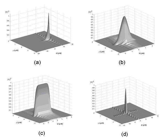
Figure 4: Frozen Waves with the on-axis longitudinal field pattern chosen as: (a) Exponential;  (b) Gaussian;  (c) Super-gaussian;  (d) Zero order  Bessel function

Another way-out exists for evaluating $S(k_{z})$, based on the assumption that

$S(k_{z})\,\simeq\,\widetilde{S}(k_{z})\;,$ (40)

which consitutes a good approximation whenever $\widetilde{S}(k_{z})$ assumes negligible values outside the interval $[-\omega_{0}/c,\ \omega_{0}/c]$.  In such a case, one can have recourse to the method associated with Eq.(28) and expand $\widetilde{S}(k_{z})$ itself in a Fourier series, getting eventually the relevant coefficients $A_{n}$ by Eq.(29).  Let us recall that it is still $K\equiv k_{z}{\rm max}-k_{z}{\rm min}=2\omega_{0}/c$.

It may be interesting to call attention to the circumstance that, when constructing FWs in terms of a sum of discrete superpositions of Bessel beams (as it was done by us in refs.[39, 40, 59, 62]), it was easy to obtain extended envelopes like, e.g., “cigars”: where easy means having recourse to few terms of the sum. By contrast, when we construct FWs —following this Section— as continuous superpositions, then it is easy to get higly localized (concentrated) envelopes.  Let us explicitly mention, moreover, that the method presented in this Section furnishes FWs that are no longer periodic along the $z$-axis (a situation that, with our old method,[39, 40, 59] was obtainable only when the periodicity interval tended to infinity).

5 The role of Special Relativity, and of Lorentz Transformations

Strict connections exist between, on one hand, the principles and structure of Special Relativity and, on the other hand, the whole subject of subluminal, luminal, superluminal Localized Waves, in the sense that it is expected since long time that a priori they are transformable one into the other via suitable Lorentz transformations (cf. refs.[1, 16, 64], besides work of ours in progress).

Let us first confine ourseves to the cases faced in this paper. Our subluminal localized pulses, that may be called “wave bullets”, behave as particles: Indeed, our subluminal pulses [as well as the luminal and superluminal (X-shaped) ones, that have been amply investigated in the past literature] do exist as solutions of any wave equations, ranging from electromagnetism and acoustics or geophysics, to elementary particle physics (and even, as we discovered recently, to gravitation physics).  From the kinematical point of view, the velocity composition relativistic law holds also for them.  The same is true, more in general, for any localized waves (pulses or beams).

Let us start for simplicity by considering, in an initial reference-frame O, just a ($\nu$-order) Bessel beam:

$$\Psi(\rho,\phi,z,t)\;=\;J_{\nu}(\rho k_{\rho})\;e^{i\nu\phi}\;e^{izk_{z}}\;e^{-i\omega t}\;.$$ (41)

In a second reference-frame O’, moving with respect to (w.r.t.) O with speed $u$ —along the positive z-axis and in the positive direction, for simplicity’s sake—, it will be observed[60] the new Bessel beam

$$\Psi(\rho^{\prime},\phi^{\prime},z^{\prime},t^{\prime})\;=\;J_{\nu}(\rho^{\prime}{k^{\prime}}_{\rho^{\prime}})\;e^{i\nu\phi^{\prime}}\;e^{iz^{\prime}{k^{\prime}}_{z^{\prime}}}\;e^{-i\omega^{\prime}t^{\prime}}\;,$$ (42)

obtained by applying the appropriate Lorentz transformation (a Lorentz “boost”) with  $\gamma=[\sqrt{1-u^{2}/c^{2}}]^{-1}$:

$${k^{\prime}}_{\rho^{\prime}}=k_{\rho};\ \ \ {k^{\prime}}_{z^{\prime}}=\gamma(k_{z}-u\omega/c^{2});\ \ \ \omega^{\prime}=\gamma(\omega-uk_{z})\;;$$ (43)

this can be easily seen, e.g., by putting

$$\rho=\rho^{\prime};\ \ \ z=\gamma(z^{\prime}+ut^{\prime});\ \ \ t=\gamma(t^{\prime}+uz^{\prime}/c^{2})$$ (44)

directly into Eq.(42).

Let us now pass[60] to subluminal pulses. We can investigate the action of a Lorentz transformation (LT), by expressing them either via the first method (Section 2) or via the second one (Section 3).  Let us consider for instance, in the frame O, a $v$-speed (subluminal) pulse, given by Eq.(3) of our Section 2.  When we go on to a second observer O’ moving with the same speed $v$ w.r.t. frame O, and, still for the sake of simplicity, passing through the origin $O$ of the initial frame at time $t=0$, the new observer O’ will see the pulse[60]

$$\Psi(\rho^{\prime},z^{\prime},t^{\prime})\;=\;e^{-it^{\prime}{\omega^{\prime}}_{0}}\,\int_{\omega_{-}}^{\omega_{+}}{\rm d}\omega\;S(\omega)\;J_{0}(\rho^{\prime}{k^{\prime}}_{\rho^{\prime}})\;e^{iz^{\prime}{k^{\prime}}_{z^{\prime}}}\;,$$ (45)

with

$${k^{\prime}}_{z^{\prime}}={\gamma}^{-1}\omega/v-\gamma b/v;\ \ \ \omega^{\prime}=\gamma b;\ \ \ {k^{\prime}}_{\rho^{\prime}}={\omega^{\prime}}_{0}/c^{2}-{{k^{\prime}}_{z^{\prime}}}^{2}\;,$$ (46)

as one gets from the Lorentz transformation in Eq.(43), or in Eq.(44), with $u=v$  [and $\gamma$ given by Eqs.(9)].  Notice that ${k^{\prime}}_{z^{\prime}}$ is a function of $\omega$, as expressed by the first one of the three relations in the previous Eqs.(46); and that here $\omega^{\prime}$ is a constant.

If we explicitly insert into Eq.(45) the relation  $\omega=\gamma(v{{k^{\prime}}_{z^{\prime}}}+\gamma b)$,  which is nothing but a re-writing of the first one of Eqs.(46), then Eq.(45) becomes[60]

$$\Psi(\rho^{\prime},z^{\prime},t^{\prime})\;=\;\gamma v\;e^{-it^{\prime}\omega_{0}}\;\int_{-\omega_{0}/c}^{\omega_{0}/c}{\rm d}{k^{\prime}}_{z^{\prime}}\;\overline{S}({k^{\prime}}_{z^{\prime}})\;J_{0}(\rho^{\prime}{k^{\prime}}_{\rho^{\prime}})\;e^{iz^{\prime}{k^{\prime}}_{z^{\prime}}}\;,$$ (47)

where $\overline{S}$ is expressed in terms of the previous function $S(\omega)$, entering Eq.(45), as follows:

$$\overline{S}({k^{\prime}}_{z^{\prime}})\;=\;S(\gamma v{k^{\prime}}_{z^{\prime}}+\gamma^{2}b)\;.$$ (48)

Equation (47) describes monochromatic beams with axial symmetry (and does coincide also with what derived within our second method, in Section 3, when posing $v=0$).

The remarkable conclusion is that a subluminal pulse, given by our Eq.(3), which appears as a $v$-speed pulse in a frame O, will appear[60] in another frame O’ (traveling w.r.t. observer O with the same speed $v$ in the same direction $z$) just as the monochromatic beam in Eq.(47) endowed with angular frequency ${\omega^{\prime}}_{0}=\gamma b$, whatever be the pulse spectral function in the initial frame O: even if the kind of monochromatic beam one arrives to does of course depend on the chosen $S(\omega)$. The vice-versa is also true, in general.

Let us set forth explicitly an observation that hasn’t been noticed in the existing literature yet. Namely, let us mention that, when starting not from Eq.(3) but from the most general solutions which —as we have already seen— are sums of solutions (3) over the various values $b_{m}$ of $b$, then a Lorentz transformation will lead us to a sum of monochromatic beams: actually, of harmonics (rather than to a single monochromatic beam).  In particular, if one wants to obtain a sum of harmonic beams, one has to apply a LT to more general subluminal pulses.

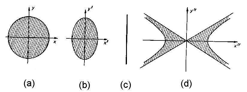
Figure 5: Let us consider an object that is intrinsically spherical, i.e., that is a sphere in its rest-frame (Panel (a)). After a generic subluminal LT along $x$, i.e., under a subluminal $x$-boost, it is predicted by Special Relativity (SR) to appear as ellipsoidal due to Lorentz contraction (Panel (b)). After a superluminal $x$-boost[16, 65, 64] (namely, when this object moves[21] with superluminal speed $V$), it is predicted by SR —in its non-restricted version (ER)— to appear[1] as in Panel (d), i.e., as occupying the cylindrically symmetric region bounded by a two-sheeted rotation hyperboloid and an indefinite double cone. The whole structure, according to ER, is expected to move rigidly and, of course, with the speed $V$, the cotangent square of the cone semi-angle being $(V/c)^{2}-1$.  Panel (c) refers to the limiting case when the boost-speed tends to $c$, either from the left or from the right (for simplicity, a space axis is skipped). It is remarkable that the shape of the localized (subluminal and superluminal) pulses, solutions to the wave equations, appears to follow the same behavior; this can have a role for a better comprehension even of de Broglie and Schroedinger wave-mechanics.  The present figure is taken from refs.[1, 16].  See also the next Figure.

Let us add that also the various superluminal localized pulses get transformed[60] one into the other by the mere application of ordinary LTs; while it may be expected that the subluminal and the superluminal LWs are to be linked (apart from some known technical difficulties, that require a particular caution) by the superluminal Lorentz ”transformations” expounded long ago, e.g., in refs.[16, 65, 64, 1] and refs. therein.  Let us recall once more that, in the years 1980-82, special relativity, in its non-restricted version, predicted that, while the simplest subluminal object is obviously a sphere (or, in the limit, a space point), the simplest superluminal object is on the contrary an X-shaped pulse (or, in the limit, a double cone): cf. Fig.5, taken from refs.[1, 16].  The circumstance that the pattern of the localized solutions to the wave equations does meet this prediction is rather interesting, and is expected to be useful —in the case, e.g., of elementary particles and quantum physics— for a deeper comprehension of de Broglie’s and Schroedinger’s wave mechanics. With regard to the fact that the simplest subluminal LWs, solutions to the wave equation, are “ball-like”, let us depict by Figs.6, in the ordinary 3D space, the general shape of the Mackinnon’s solutions as expressed by Eq.(10) for $v<<c$: In such figures we graphically represent the field iso-intensity surfaces, which in the considered case result to be (as expected) just spherical.

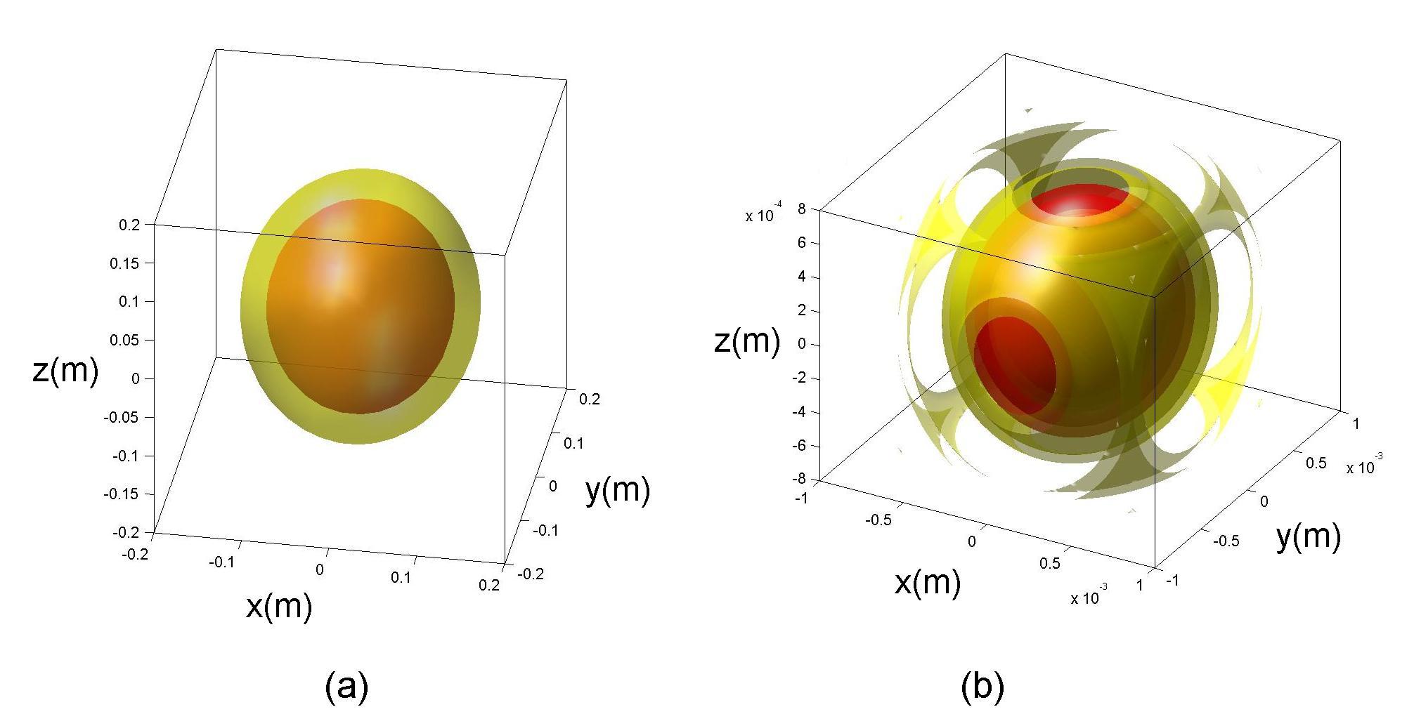
Figure 6: In the previous Figure we have seen how SR, in its non-restricted version (ER), predicted[1, 16] that, while the simplest subluminal object is obviously a shere (or, in the limit, a space point), the simplest superluminal object is on the contrary an X-shaped pulse (or, in the limit, a double cone).  The circumstance that the Localized Solutions to the wave equations do follow the same pattern is rather interesting, and is expected to be useful —in the case, e.g., of elementary particles and quantum physics— for a deeper comprehension of de Broglie’s and Schroedinger’s wave mechanics. With regard to the fact that the simplest subluminal LWs, solutions to the wave equations, are “ball-like”, let us depict by these figures, in the ordinary 3D space, the general shape of the Mackinnon’s solutions as expressed by Eq.(10), numerically evaluated for $v<<c$. In figures (a) and (b) we graphically represent the field iso-intensity surfaces, which in the considered case result to be (as expected) just spherical.

We have also seen, among the others, that, even if our first method (Section 2) cannot yield directly zero-speed envelopes, such envelopes “at rest”, in Eq.(31), can be however obtained by applying a $v$-speed LT to eq.(16). In this way, one starts from many frequencies [Eq.(16)] and ends up with one frequency only [Eq.(31)], since $b$ gets transformed into the frequency of the monochromatic beam.

6 Non-axially symmetric solutions: The case of higher-order Bessel beams

Let us stress that till now we have paid attention to exact solutions representing axially-symmetric (subluminal) pulses only: that is to say, to pulses obtained by suitable superpositions of zero-order Bessel beams.

It is however interesting to look also for analytic solutions representing non-axially symmetric subluminal pulses, which can be constructed in terms of superpositions of $\nu$-order Bessel beams, with $\nu$ a positive integer ($\nu>0$).  This can be attempted both in the case of Sect.2 (first method), and in the case of Sect.3 (second method).

For brevity’s sake, let us take only the first methos (Sect.2) into consideration.  One is immediately confronted with the difficulty that no exact solution is known for the integral in Eq.(8) when $J_{0}(.)$ is replaced with $J_{\nu}(.)$.

One can overcome this difficulty by following a simple method, which will allow us to obtain “higher-order” subluminal waves in terms of the axially-symmetric ones.  Indeed, it is well-known that, if $\Psi(x,y,z,t)$ is an exact solution to the ordinary wave equation, then  $\partial^{n}\Psi/\partial x^{n}$  and  $\partial^{n}\Psi/\partial y^{n}$  are also exact solutions.  One should notice that, on the contrary, when working in cylindrical co-ordinates, if $\Psi(\rho,\phi,z,t)$ is a solution to the wave equation, $\partial\Psi/\partial\rho$  and  $\partial\Psi/\partial\phi$ are not solutions, in general.  Nevertheless, it is not difficult at all to reach the noticeable conclusion that, once  $\Psi(\rho,\phi,z,t)$  is a solution, then also

$$\overline{\Psi}(\rho,\phi,z,t)\;=\;e^{i\phi}\left(\frac{\partial\Psi}{\partial\rho}+\frac{i}{\rho}\frac{\partial\Psi}{\partial\phi}\right)$$ (49)

is an exact solution. For example, for an axially-symmetric solution of the type $\Psi=J_{0}(k_{\rho}\rho)\,\exp[ik_{z}]\,\exp[-i\omega t]$, equation (49) yields $\overline{\Psi}=-k_{\rho}\,J_{1}(k_{\rho}\rho)\,\exp[i\phi]\,\exp[ik_{z}]\,\exp[-i\omega t]$, which is actually another analytic solution.

In other words, it is enough to start for simplicity from a zero-order Bessel beam, and to apply Eq.(49), successively, $\nu$ times, in order to get as a new solution  $\overline{\Psi}=(-k_{\rho})^{\nu}\,J_{\nu}(k_{\rho}\rho)\,\exp[i\nu\phi]\,\exp[ik_{z}]\,\exp[-i\omega t]$, which is a $\nu$-order Bessel beam.

In such a way, when applying $\nu$ times Eq.(49) to the (axially-symmetric) subluminal solution $\Psi(\rho,z,t)$ in Eqs.(16,15,14)  [obtained from Eq.(3) with spectral function $S(\omega)$], we are able to get the subluminal non-axially symmetric pulses  $\Psi_{\nu}(\rho,\phi,z,t)$  as new analytic solutions, consisting as expected in superpositions of $\nu$-order Bessel beams:

$$\Psi_{n}(\rho,\phi,z,t)\;=\;\int_{\omega_{-}}^{\omega_{+}}{\rm d}\omega\;S^{\prime}(\omega)\;J_{\nu}(k_{\rho}\rho)\;e^{i\nu\phi}\;e^{ik_{z}z}\;e^{-i\omega t}\;,$$ (50)

with $k_{\rho}(\omega)$ given by Eq.(4), and quantities $S^{\prime}(\omega)=(-k_{\rho}(\omega))^{\nu}S(\omega)$ being the spectra of the new pulses.  If $S(\omega)$ is centered at a certain carrier frequency (it is a gaussian spectrum, for instance), then $S^{\prime}(\omega)$ too will approximately be of the same type.

Now, if we wish the new solution $\Psi_{\nu}(\rho,\phi,z,t)$ to possess a pre-defined spectrum $S^{\prime}(\omega)=F(\omega)$, we can first take Eq.(3) and put  $S(\omega)=F(\omega)/(-k_{\rho}(\omega))^{\nu}$  in its solution (16), and afterwards apply to it, $\nu$ times, the operator  $U\equiv\exp[i\phi]\;[\partial/\partial\rho+(i/\rho)\partial/\partial\phi)]\,$:  As a result, we will obtain the desired pulse, $\Psi_{\nu}(\rho,\phi,z,t)$, endowed with $S^{\prime}(\omega)=F(\omega)$.

An example:

On starting from the subluminal axially-symmetric pulse $\Psi(\rho,z,t)$, given by Eq.(16) with the gaussian spectrum (17), we can get the subluminal, non-axially symmetric, exact solution $\Psi_{1}(\rho,\phi,z,t)$ by simply calculating

$$\Psi_{1}(\rho,\phi,z,t)\;=\;{{\partial\Psi}\over{\partial\rho}}\ \;e^{i\phi}\;,$$ (51)

which actually yields the “first-order” pulse $\Psi_{1}(\rho,\phi,z,t)$, which can be more compactly written in the form:

$$\Psi_{1}(\rho,\phi,\eta,\zeta)\;=\;2\,{b\over c}\,v\,\gamma^{2}\;{\exp{\left[i{b\over c}\,\beta\,\gamma^{2}\;\eta\right]}}\sum_{n=-\infty}^{\infty}\;A_{n}\;\exp{[in{\pi\over\beta}]}\ \;\psi_{1n}$$ (52)

with

$$\psi_{1n}(\rho,\phi,\eta,\zeta)\equiv\displaystyle{{b^{2}\over c^{2}}\,\gamma^{2}\rho\ \;Z^{-3}\ [Z\,\cos Z-\sin Z]\ \;e^{i\phi}}\;,$$ (53)

where

$$Z\equiv\displaystyle{\sqrt{{b^{2}\over c^{2}}\,\gamma^{2}\rho^{2}+\left({b\over c}\,\gamma^{2}\zeta+n\pi\right)^{2}}}\;.$$ (54)

This exact solution, let us repeat, corresponds to superposition (50),  with  $S^{\prime}(\omega)=k_{\rho}(\omega)S(\omega)$,  quantity $S(\omega)$ being given by Eq.(17).  It is represented in Figure 7. The pulse intensity has a “donut-like” shape.

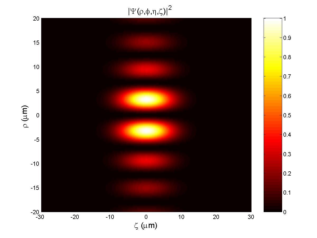
Figure 7: Orthogonal projection of the field intensity corresponding to the higher order subluminal pulse represented by the exact solution Eq.(51), quantity $\Psi$ being given by Eq.(16) with the gaussian spectrum (17). The pulse intensity happens to have this time a “donut”-like shape.

7 Conclusions

Like in the well-known superluminal case, the (more orthodox, in a sense) subluminal Localized Waves can be obtained by suitable superpositions of Bessel beams. They had been till now almost neglected, however, for the mathematical difficulties met in finding out analytic expressions for them, difficulties associated with the fact that the superposition integral runs over a finite interval. We have re-addressed in this paper the question of such subluminal LWs, obtaining by contrast, and in a simple way, non-diffracting subluminal pulses as exact analytic solutions to the wave equations. Such new ideal subluminal solutions —which propagate without distortion in any homogeneous linear medium— have been herein obtained for arbitrarily chosen frequencies and bandwidths, avoiding in particular any recourse to the non-causal components so frequently plaguing the previously known localized waves.

Indeed, only one closed-form subluminal LW solution, $\psi_{\rm cf}$, to the wave equations was known[3]: the one obtained by choosing in the relevant integration a constant weight-function $S(\omega)$; while all other solutions had been got in the past only via numerical simulations. By contrast, we have shown above, for instance, that a subluminal LW can be obtained in closed form by adopting any spectra $S(\omega)$ that be expansions in terms of $\psi_{\rm cf}$.  In fact, the initial disadvantage of the subluminal case, that of being associated with a a limited bandwidth, has been turned into an advantage, since in the case of “truncated” integrals —at variance with the superluminal case— the spectrum $S(\omega)$ can be expanded in a Fourier series.

More in general, it has been shown in what precedes how can one arrive at exact solutions both by integration over the Bessel beams’ angular frequency $\omega$, and by integration over their longitudinal wavenumber $k_{z}$. Both methods are expounded in this paper. The first one appears to be powerful enough; we have studied the second method as well, however, since it allows dealing even with the limiting case of zero-speed solutions (thus furnishing a new way, in terms of continuous spectra, for obtaining the so-called “Frozen Waves”, so promising also from the point of view of applications).   We have briefly treated the case, moreover, of non axially-symmetric solutions, namely, of higher order Bessel beams.

At last, attention has been always paid to the role of Special Relativity, and to the fact that the localized waves are transformed one into the other by suitable Lorentz Transformations. Moreover, our results seem to show that in the subluminal case the simplest LW solutions are (for $v<<c$) “ball”-like, as expected since long[1] on the mere basis of special relativity[16]. Actually, already in the years 1980-82 it had been predicted that, if the simplest subluminal object is a sphere (or, in the limit, a space point), then the simplest superluminal object is an X-shaped pulse (or, in the limit, a double-cone); and viceversa: Cf. Fig.5, taken from ref.[1]. It is rather interesting that the same pattern appears to be followed by the localized solutions of the wave equations. For the subluminal case, see. e.g., Figs.6.

The localized pulses, endowed with a finite energy, or merely truncated, will be constructed in another paper.

In the present work we have fixed our attention especially on electromagnetism and optics: but results of the same kind are valid whenever an essential role is played by a wave-equation (like in acoustics, seismology, geophysics, gravitation, elementary particle physics, etc.).

8 Acknowledgements

The authors are indebted to H.E. Hernández-Figueroa for his continuous collaboration, and thank I.M.Besieris, A.Castoldi, C.Conti, J-y.Lu, G.C.Maccarini, R.Riva, P.Saari, A.M.Shaarawi, M.Tygel for useful discussions or kind interest.

References

- [1] A.O.Barut, G.D.Maccarrone and E.Recami: “On the shape of tachyons”, Nuovo Cimento A71 (1982) 509-533; and refs. therein.
- [2] R.Grunwald, U.Griebner, U.Neumann and V.Kebbel, “Self-recontruction of ultrashort-pulse Bessel-like X-waves”, CLEO/QELS Conference (San Francisco; 2004), paper no.CMQ7.
- [3] L. Mackinnon: “A nondispersive de Broglie wave packet”, Found. Phys. 8 (1978) 157.
- [4] Localized Waves: Theory and Applications, ed. by H.E.Hernández-Figueroa, M.Zamboni-Rached, and E.Recami (J.Wiley; New York, 2007), in press.
- [5] E.Recami, M.Zamboni-Rached and H.E.Hernández-Figueroa: “Localized waves: A historical and scientific introduction”, introductory Chapter of the book in ref.[4].
- [6] M.Zamboni-Rached, E.Recami and H.E.Hernández-Figueroa: “Structure of the nondiffracting waves, and some interesting applications”, a Chapter of the book in ref.[4].
- [7] S.Longhi: “Spatial-temporal Gauss-Laguerre waves in dispersive media”, Phys. Rev. E68 (2003) no.066612 [6 pages].
- [8] A.M.Shaarawi, I.M.Besieris and T.M.Said, “Temporal focusing by use of composite X-waves”, J. Opt. Soc. Am. A20 (2003) 1658-1665.
- [9] I.M.Besieris, M.Abdel-Rahman, A.Shaarawi and A.Chatzipetros: “Two fundamental representations of localized pulse solutions of the scalar wave equation”, Progress in Electromagnetic Research (PIER) 19 (1998) 1-48.
- [10] M.Zamboni-Rached and H.E.Hernàndez-Figueroa: “A rigorous analysis of Localized Wave propagation in optical fibers”, Opt. Comm. 191 (2000) 49-54.
- [11] I.Besieris and A.Shaarawi, “Paraxial localized waves in free space”, Opt. Express 12 (2004) 3848-3864.
- [12] R.Donnelly and R.W.Ziolkowski, “Designing localized waves”, Proc. R. Soc. Lond. A440 (1993) 541-565.
- [13] C.A.Dartora, M.Z.Rached and E.Recami: “General formulation for the analysis of scalar diffraction-free beams using angular modulation: Mathieu and Bessel beams”, Optics Communications 222 (2003) 75-85.
- [14] J.Salo and M.M.Salomaa: “Subsonic nondiffracting waves”, Acoustics Res. Lett. Online 2(1) (2001) 31-36.
- [15] S.Longhi: “Localized subluminal envelope pulses in dispersive media”, Opt. Lett. 29 (2004) 147-149.
- [16] E.Recami: “Classical Tachyons and Possible Applications”, Rivista Nuovo Cim. 9(6) (1986) 1–178, issue no.6; and refs. therein.
- [17] C.Conti, S.Trillo, G.Valiulis, A.Piskarkas, O. van Jedrkiewicz, J.Trull and P.Di Trapani: “Non-linear electromagnetic X-waves”, Phys. Rev. Lett. 90 (2003) 170406.
- [18] M.Zamboni-Rached: “Localized solutions: Structure and Applications”, M.Sc. thesis (Phys. Dept., Campinas State University, 1999); and also M.Zamboni-Rached, “Localized waves in diffractive/dispersive media”, PhD Thesis, Aug.2004, Universidade Estadual de Campinas, DMO/FEEC [download at http://libdigi.unicamp.br/document/?code=vtls000337794], and refs. therein.
- [19] R.Courant and D.Hilbert: Methods of Mathematical Physics, vol.2, p.760 (J.Wiley; New York, 1966).
- [20] H.Bateman: Electrical and Optical Wave Motion (Cambridge Univ.Press; Cambridge, 1915).
- [21] E.Recami, M.Zamboni-Rached and C.A.Dartora: “The X-shaped, localized field generated by a Superluminal electric charge” Physical Review E69 (2004) no.027602 [4 pages].
- [22] J.-y. Lu and J.F.Greenleaf: “Nondiffracting X-waves: Exact solutions to free-space scalar wave equation and their finite aperture realizations”, IEEE Transactions in Ultrasonics Ferroelectricity and Frequency Control 39 (1992) 19-31; and refs. therein.
- [23] E.Recami: “On localized X-shaped Superluminal solutions to Maxwell equations”, Physica A252 (1998) 586-610; and refs. therein.
- [24] J.-y. Lu and J.F.Greenleaf: “Experimental verification of nondiffracting X-waves”, IEEE Transactions in Ultrasonics Ferroelectricity and Frequency Control 39 (1992) 441-446.
- [25] H.Sõnajalg, P.Saari, “Suppression of temporal spread of ultrashort pulses in dispersive media by Bessel beam generators”, Opt. Letters 21 (1996) 1162-1164. Cf. also H.Sõnajalg, M.Rätsep and P.Saari: Opt. Lett. 22 (1997) 310.
- [26] P.Saari and K.Reivelt: “Evidence of X-shaped propagation-invariant localized light waves”, Physical Review Letters 79 (1997) 4135-4138. Cf. also H.Valtua, K.Reivelt and P.Saari: “Methods for generating wideband localized waves of superluminal group-velocity”, Opt. Comm. 278 (2007) 1-7.
- [27] D.Mugnai, A.Ranfagni, and R.Ruggeri: “Observation of Superluminal behaviors in wave propagation”, Physical Review Letters 84 (2000) 4830-4833.
- [28] J.-y. Lu, H.-H.Zou and J.F.Greenleaf: “Biomedical ultrasound beam forming”, Ultrasound in Medicine and Biology 20 (1994) 403-428.
- [29] J.-y. Lu, H.-h.Zou and J.F.Greenleaf: “Producing deep depth of field and depth independent resolution in NDE with limited diffraction beams”, Ultrasonic Imaging 15 (1993) 134-149.
- [30] J.-y. Lu and J.F.Greenleaf: “Comparison of sidelobes of limited diffraction beams and localized waves”, in Acoustic Imaging, vol.21, ed. by J.P.Jones (Plenum; New York, 1995), pp.145-152-
- [31] R.W.Ziolkowski: “Localized transmission of electromagnetic energy”, Physical Review A39 (1989) 2005-2033.
- [32] I.M.Besieris, A.M.Shaarawi and R.W.Ziolkowski: “A bi-directional traveling plane wave representation of exact solutions of the scalar wave equation”, J. Math. Phys. 30 (1989) 1254-1269.
- [33] R.W.Ziolkowski: “Localized wave physics and engineering”, Physical Review A44 (1991) 3960-3984.
- [34] : “Classical solutions of Maxwell’s equations with group-velocity different from , and the photon tunneling effect”, Phys. Lett. A225 (1997) 203-209.
- [35] W.Ziolkowski, I.M.Besieris and A.M.Shaarawi: “Aperture realizations of exact solutions to homogeneous wave-equations”, J. Opt. Soc. Am. A10 (1993) 75.
- [36] J.Durnin, J.J.Miceli and J.H.Eberly: “Diffraction-free beams”, Physical Review Letters 58 (1987) 1499-1501.
- [37] J.Durnin: “Exact solutions for nondiffracting beams: I. The scalar theory”, Journal of the Optical Society of America A4 (1987) 651-654.
- [38] M.Zamboni-Rached, E.Recami and H.E.Hernández-Figueroa: “New localized Superluminal solutions to the wave equations with finite total energies and arbitrary frequencies”, European Physical Journal D21 (2002) 217-228.
- [39] M.Zamboni-Rached: “Stationary optical wave fields with arbitrary longitudinal shape by superposing equal frequency Bessel beams: Frozen Waves”, Optics Express 12 (2004) 4001-4006.
- [40] M.Zamboni-Rached, E.Recami and H.E.Hernández-Figueroa: “Theory of ‘Frozen Waves’: Modeling the shape of stationary wave fields”, Journal of the Optical Society of America A11 (2005) 2465-2475.
- [41] J.N.Brittingham: “Focus wave modes in homogeneous Maxwell’s equations: transverse electric mode”, J. Appl. Phys. 54 (1983) 1179-1189.
- [42] A.Sezginer: “A general formulation of focus wave modes”, J. Appl. Phys. 57 (1985) 678-683.
- [43] E.Recami, M.Zamboni-Rached, K.Z.Nobrega, C.A.Dartora and H.E.Hernández-Figueroa: “On the Localized Superluminal Solutions to the Maxwell Equations”, IEEE Journal of Selected Topics in Quantum Electronics 9 (2003) 59-73.
- [44] E.Recami: “Superluminal motions? A bird’s-eye view of the experimental status-of-the-art”, Found. Phys. 31 (2001) 1119-1135.
- [45] J.Salo, J.Fagerholm, A.T.Friberg and M.M.Salomaa: “Nondiffracting bulk-acoustic X-waves in crystals”, Phys. Rev. Lett. 83 (1999) 1171-1174.
- [46] A.T.Friberg, J.Fagerholm and M.M.Salomaa: “Space-frequency analysis of nondiffracting pulses”, Optics Communications 136 (1997) 207-212.
- [47] A.M.Shaarawi and I.M.Besieris: “On the Superluminal propagation of X-shaped localized waves”, J. Phys. A33 (2000) 7227-7254.
- [48] M.Zamboni-Rached, K.Z.Nobrega, H.E.Hernández-Figueroa and E.Recami: “Localized Superluminal solutions to the wave equation in (vacuum or) dispersive media, for arbitrary frequencies and with adjustable bandwidth”, Optics Communications 226 (2003) 15-23.
- [49] M.A.Porras, G.Valiulis and P.Di Trapani: “Unified description of Bessel X waves with cone dispersion and tilted pulses”, ¡Phys. Rev. E68 (2003) 016613.
- [50] M.A.Porras, S.Trillo, C.Conti and P.Di Trapani: “Paraxial envelope X waves”, Opt. Lett. 28 (2003) 1090-1092.
- [51] M.Zamboni-Rached, E.Recami and F.Fontana: “Localized Superluminal solutions to Maxwell equations propagating along a normal-sized waveguide”, Physical Review E64 (2001) no.066603 [6 pages].
- [52] M.Zamboni-Rached, K.Z.Nobrega, E.Recami and H.E.Hernández-Figueroa: “Superluminal X-shaped beams propagating without distortion along a coaxial guide”, Physical Review E66 (2002) no.036620 [10 pages]; and refs. therein.
- [53] M.Zamboni-Rached, F.Fontana and E.Recami: “Superluminal localized solutions to Maxwell equations propagating along a waveguide: The finite-energy case”, Phys. Rev. E67 (2003) no.036620 [7 pages].
- [54] M.Zamboni-Rached, A.Shaarawi and E.Recami: “Focused X-Shaped Pulses”, Journal of the Optical Society of America A21 (2004) 1564-1574.
- [55] Z.Bouchal, J.Wagner and M.Chlup: “Self-reconstruction of a distorted nondiffracting beam”, Optics Communications 151 (1998) 207-211.
- [56] A.P.L.Barbero, H.E.Hernández F., and E.Recami: “On the propagation speed of evanescent modes”, Phys. Rev. E62 (2000) 8628, and refs. therein.
- [57] M. Zamboni-Rached, H. E. Hernández-Figueroa and E.Recami: “Chirped optical X-shaped pulses in material media”, J. Opt. Soc. Am. A21 (2004) 2455-2463.
- [58] A.C.Newell and J.V.Molone: Nonlinear Optics (Addison & Wesley; Redwood City, CA, 1992).
- [59] M.Zamboni-Rached: “Diffraction-attenuation resistant beams in absorbing media”, Opt. Express 14 (2006) 1804-1809 [paper chosen for mention also in the Virtual Journal for Biomedical Optics, and in Laser Focus World, Section “new bracks”].
- [60] P.Saari and K.Reivelt: “Generation and classification of localized waves by Lorentz transformations in Fourier space”, Phys. Rev. E69 (2004) 036612; and refs. therein.
- [61] M. Zamboni-Rached: “Analytical expressions for the longitudinal evolution of nondiffracting pulses truncated by finite apertures,” J. Opt. Soc. Am. A23 (2006) 2166-2176.
- [62] M.Zamboni-Rached, E.Recami, et al.: “Method and apparatus for producing stationary intense wavefields of arbitrary shape”, application/patent nos. 05743093.6-1240/EP2005052352 (initially filed c/o the E.P.O. on 23.05.05).
- [63] W.A.Rodrigues, J.Vaz and E.Recami: “Free Maxwell equations, Dirac equation, and non-dispersive de Broglie wave packets”, in Courants, Amers, Écueils en Microphysique, ed. by G. & P.Lochak (Paris, 1994), pp.379-392.
- [64] R.Mignani and E.Recami: “Generalized Lorentz Transformations and Superluminal Objects in Four Dimensions”, Nuovo Cimento A14 (1973) 169-189; A16, 206.
- [65] E.Recami and W.A.Rodrigues: “A Model Theory for Tachyons in Two Dimensions”, in Gravitational Radiation and Relativity (vol.3 of the Proceedings of the Sir Arthur Eddington Centenary Symposium), ed. by J.Weber & T.M.Karade (World Scientific; Singapore, 1985), pp.151-203.