Cheon’s anholonomies in Floquet operators

Abstract

Anholonomies in the parametric dependences of the eigenvalues and the eigenvectors of Floquet operators that describe unit time evolutions of periodically driven systems, e.g., kicked rotors, are studied. First, an example of the anholonomies induced by a periodically pulsed rank-1 perturbation is given. As a function of the strength of the perturbation, the perturbed Floquet operator of the quantum map and its spectrum are shown to have a period. However, we show examples where each eigenvalue does not obey the periodicity of the perturbed Floquet operator and exhibits an anholonomy. Furthermore, this induces another anholonomy in the eigenspaces, i.e., the directions of the eigenvectors, of the Floquet operator. These two anholonomies are previously observed in a family of Hamiltonians [T. Cheon, Phys. Lett. A 248, 285 (1998)] and are different from the phase anholonomy known as geometric phases. Second, the stability of Cheon’s anholonomies in periodically driven systems is established by a geometrical analysis of the family of Floquet operators. Accordingly, Cheon’s anholonomies are expected to be abundant in systems whose time evolutions are described by Floquet operators. As an application, a design principle for quantum state manipulations along adiabatic passages is explained.

I Introduction

The parametric dependence of an eigenvector of an operator often exhibits anholonomy in its phase  GeometricPhaseReview . A simple demonstration of the phase anholonomy in an eigenvector of a Hamiltonian is shown by Berry Berry:PRSLA-430-405 : Prepare the system to be in an eigenstate of the Hamiltonian, whose energy spectrum is assumed to be discrete and nondegenerate. During the adiabatic change of the parameters of the Hamiltonian, which is kept to be nondegenerate along the change, the system continuously remains to be in an eigenstate of the instantaneous Hamiltonian, according to the adiabatic theorem Born:ZP-51-165 . When the parameter returns to its initial value, after the adiabatic change along a closed path in the parameter space, the difference between the initial and the final state vectors is only in its phase, which is composed by two ingredients: One is called a dynamical phase that is determined by the accumulation of the eigenenergy along the adiabatic time evolution. The other is called a geometric phase, or the phase anholonomy that reflects the geometric structure of the family of eigenvectors in the parameter space. There is a non-Abelian generalization of the phase anholonomy: This was pointed out by Wilczek and Zee in the parametric change of an eigenspace of a Hamiltonian that has a spectral degeneracy Wilczek:PRL-52-2111 . The phase anholonomy appears in various fields of physics, besides quantum mechanics, and brings profound consequences GeometricPhaseReview .

Recently, Cheon found exotic anholonomies, which are completely different from the conventional phase anholonomy, in a family of systems with generalized pointlike potentials Cheon:PLA-248-285 . Cheon’s anholonomies appear, surprisingly, both in eigenenergies and eigenvectors: The trail of an eigenenergy along a change of parameters on a closed path that encircles a singularity does not draw a closed curve but, instead, a spiral. Since the initial and the final eigenenergies in the closed path are different eigenvalues of a Hermite operator, the corresponding eigenvectors must be orthogonal. Hence the eigenenergy anholonomy induces another anholonomy in the direction of eigenvectors. The origin of Cheon’s anholonomies in the family of systems with the generalized pointlike potentials is identified with the geometrical structure of the family’s parameter space Cheon:AP-294-1 ; Tsutsui:JMP-42-5687 .

In order to distinguish Cheon’s anholonomy in the directions of eigenvectors from Wilczek-Zee’s phase anholonomy, which requires a degenerate spectrum and transports an eigenvector into its nonorthogonal direction in general along adiabatic changes on closed paths, we will call the former an eigenspace anholonomy: Wilczek-Zee’s phase anholonomy concerns the change of an eigenvector within a single and degenerate eigenspace and Cheon’s eigenspace anholonomy, which do not require spectral degeneracies, concerns the journey of an eigenvector from one eigenspace into another eigenspace.

We can easily expect that Cheon’s anholonomies would bring profound consequences in various fields of physics, as is done by the phase anholonomy. For example, in the adiabatic (sometimes referred to as Born-Oppenheimer Born:AP-84-457 ) approximation Born:1954 , it has been considered to be legitimate to assume that an adiabatic potential surface, which is an eigenvalue of an electronic Hamiltonian with a frozen nuclear configuration, is a single-valued function of the nuclear configuration. The single-valuedness would be broken if Cheon’s eigenenergy anholonomy emerged. A similar question may be raised in the Bloch theory in solid state physics Kittel:ISSP . At the same time, Cheon’s anholonomies may be applied to manipulate quantum systems to transfer a quantum state adiabatically into another state, as is suggested by Cheon Cheon:PLA-248-285 . The last point will be discussed more precisely in this paper. However, all known examples of the eigenenergy anholonomy, up to now, require an exotic connection condition around a singular potential Tsutui:JPA-36-275 . Hence it is still worth to find systems that exhibit Cheon’s anholonomies.

The purpose of the present paper is to show Cheon’s anholonomies in periodically driven systems. More precisely, we will discuss quasienergy and eigenspace anholonomies with respect to Floquet operators that describe unit time evolutions of the periodically driven systems. First, we provide an instance of a quantum map, i.e., a quantum system under a periodically pulsed perturbation QuantumMap . The simplicity of the Floquet operators of quantum maps allows us a thorough analysis. In order to prepare it, the parametric dependence, induced by the change of the strength of the perturbation, of eigenvectors of the Floquet operators of quantum maps is reviewed in Section II. In Section III, a quantum map that is perturbed by a rank-$1$ operator is introduced. The details of its properties are explained in Appendices A and B. In Section IV, it is shown that the rank-$1$ perturbation, with respect to the original Floquet operator, enables us to introduce a family of Floquet operators to realize Cheon’s anholonomies. Several examples are shown in SectionV. Second, the stability of the anholonomies is examined. A geometrical analysis, which is shown in Section VI, of the family of Floquet operators elucidates that the appearance of Cheon’s anholonomies is not restricted in the periodically pulsed systems and is also possible in periodically driven systems in general. Furthermore, we may claim that Cheon’s anholonomies are abundant in systems whose time evolutions are described by Floquet operators. Among possible consequences and applications of our result, Section VII provides a discussion on a design principle on quantum state manipulations along adiabatic passages. Section VIII provides a discussion and a summary. A part of the present result was briefly announced in Ref. TM061 .

II Adiabatic transport of eigenvectors in a quantum map

To prepare our analysis of quantum maps, we review the parametric motions of eigenvectors and eigenvalues of Floquet operators and the adiabatic theorem for periodically driven systems. Let us consider a periodically pulsed driven system (with a period $T$) described by the “kicked” Hamiltonian:

$$\hat{H}(t)=\hat{H}_{0}+\lambda\hat{V}\sum_{n\in\mathbb{Z}}\delta(t-nT),$$ (1)

where $\hat{H}_{0}$ and $\hat{V}$ describe the “free” motion and the pulsed perturbation, respectively, and $\lambda$ is the strength of the perturbation. In the following, we focus on the stroboscopic description of the state vector $|{}\psi_{n}{}\rangle$ at $t=nT-0$. The time evolution of $|{}\psi_{n}{}\rangle$ is described by the quantum map $|{}\psi_{n+1}{}\rangle=\hat{U}_{\lambda}|{}\psi_{n}{}\rangle$, where

$$\hat{U}_{\lambda}=e^{-i\hat{H}_{0}T/\hbar}e^{-i\lambda\hat{V}/\hbar}$$ (2)

is a Floquet operator QuantumMap . In the following, we set $\hbar=1$. In order to show a simple example of the parametric motions of eigenvalues and eigenvectors, we assume that the spectrum of $\hat{U}_{\lambda}$ contains only discrete components and has no degeneracy. At the same time, in order to avoid subtle issues that are brought from the infinite dimensionality of the Hilbert space $\mathcal{H}$ endnote:infinite , we assume that $N\equiv\dim\mathcal{H}$ is finite. This assumption does no harm to the descriptions of many systems where an appropriate introduction of the truncation of the Hilbert space is feasible.

Since $\hat{U}_{\lambda}$ (2) is unitary, its eigenvalues $\{z_{n}(\lambda)\}_{n=0}^{N-1}$ are complex and on the unit circle, i.e., $|z_{n}(\lambda)|=1$. The phase of $z_{n}(\lambda)$ indicates the increment of the dynamical phase during the unit time evolution whose initial state is the corresponding eigenstate $|{}\xi_{n}(\lambda){}\rangle$. The time-average of the dynamical phase determines a quasienergy $E_{n}(\lambda)=-T^{-1}{\rm Im}[\ln z_{n}(\lambda)]$ (or, $z_{n}(\lambda)=e^{-iE_{n}(\lambda)T}$). Note that the value of quasienergy has an ambiguity because of the period $2\pi/T$ in the quasienergy space. We remark that the eigenvalue equation

$$\hat{U}_{\lambda}|{}\xi_{n}(\lambda){}\rangle=z_{n}(\lambda)|{}\xi_{n}(\lambda){}\rangle$$ (3)

determines the eigenvalue and the eigenvector only pointwise in $\lambda$. By assuming the continuity about $\lambda$, we obtain the derivatives of $E_{n}(\lambda)$ and $|{}\xi_{n}(\lambda){}\rangle$ Nakamura:PRA-35-5294 :

$$\frac{\partial}{\partial\lambda}E_{n}(\lambda) = \frac{1}{T}\langle{}\xi_{n}(\lambda){}|{}\hat{V}{}|{}\xi_{n}(\lambda){}\rangle,$$ (4)

$$\frac{\partial}{\partial\lambda}|{}\xi_{n}(\lambda){}\rangle = -iA_{n}(\lambda)|{}\xi_{n}(\lambda){}\rangle$$

$${}+i\sum_{m\neq n}\frac{z_{m}(\lambda)\langle{}\xi_{m}(\lambda){}|{}\hat{V}{}|{}\xi_{n}(\lambda){}\rangle}{z_{m}(\lambda)-z_{n}(\lambda)}|{}\xi_{m}(\lambda){}\rangle,$$

where $|{}\xi_{n}(\lambda){}\rangle$ is assumed to be normalized and $A_{n}(\lambda)\equiv i\langle{}\xi_{n}(\lambda){}|\partial|{}\xi_{n}(\lambda){}\rangle/\partial\lambda$ is a geometric gauge potential Mead:JCP-70-2284 . These derivatives compose a set of equations of motion for a virtual time $\lambda$ endnote:leveldynamics . With a given “initial condition” of $\{E_{n}(\lambda),|{}\xi_{n}(\lambda){}\rangle\}_{n}$, at $\lambda=\lambda_{0}$, we may integrate the equations of motion (4) and (II). Note that, under the presence of anholonomy GeometricPhaseReview , the single-valuedness of the solution $\{E_{n}(\lambda),|{}\xi_{n}(\lambda){}\rangle\}_{n}$ generally holds only locally in the parameter space of $\lambda$.

The adiabatic theorem Born:ZP-51-165 for periodically driven systems Holthaus:PRL-69-1596 provides a physical significance of the geometry (i.e., $\lambda$-dependence) of $|{}\xi_{n}(\lambda){}\rangle$. Note that the parameter $\lambda$, which is supposed to be slowly changed, is the strength of the perturbation that is applied periodically: $\lambda$ will be changed from $\lambda_{\rm i}$ to $\lambda_{\rm f}$, during the $M$ steps, where the corresponding time interval is $TM$. Let $\lambda_{j}$ be the value of $\lambda$ at the $j$-th step ($0\leq j\leq M$). In particular $\lambda_{0}=\lambda_{\rm i}$ and $\lambda_{M}=\lambda_{\rm f}$. The slowness of the change of the parameter is expressed by the condition $\lambda_{j+1}-\lambda_{j}=\mathcal{O}(M^{-1})$ as $M\to\infty$. We start with an initial condition that, at $\lambda=\lambda_{\rm i}$, the system is in an eigenstate $|{}\xi_{n}(\lambda_{\rm i}){}\rangle$ of $\hat{U}_{\lambda_{\rm i}}$. The final state $|{}\Psi_{\rm f}{}\rangle$ is

$$|{}\Psi_{\rm f}{}\rangle\equiv\mathop{\mathcal{T}}_{\leftarrow}\left[\prod_{j=1}^{M}\hat{U}_{\lambda_{j}}\right]|{}\xi_{n}(\lambda_{\rm i}){}\rangle,$$ (6)

where $\mathop{\mathcal{T}}_{\leftarrow}$ represents a time-orderd (or, equivalently, path-orderd) product. According to the adiabatic theorem, the final state will converge to $|{}\xi_{n}(\lambda_{\rm f}){}\rangle$ as $M\to\infty$, except its phase. In the following, we will evaluate the phase of the final state. From the equation of motion (II), we have

$$\begin{split}&\hat{U}_{\lambda}|{}\xi_{n}(\lambda-\delta){}\rangle\\ &=\exp\left\{-iE_{n}(\lambda)T+iA_{n}(\lambda)\delta\right\}|{}\xi_{n}(\lambda){}\rangle\\ &\quad-\sum_{m\neq n}\frac{iz_{m}(\lambda)^{2}\langle{}\xi_{m}(\lambda){}|\hat{V}|{}\xi_{n}(\lambda){}\rangle\delta}{z_{m}(\lambda)-z_{n}(\lambda)}|{}\xi_{m}(\lambda){}\rangle+\mathcal{O}(\delta^{2})\end{split}$$ (7)

as $\delta\to 0$. According to the adiabatic theorem Holthaus:PRL-69-1596 , we need only the first term above for the evaluation of the phase. Hence we have

$$|{}\Psi_{\rm f}{}\rangle\simeq\exp\left\{-i\sum_{j=1}^{M}E_{n}(\lambda_{j})T+i\int_{\lambda_{\rm i}}^{\lambda_{\rm f}}A_{n}(\lambda)d\lambda\right\}|{}\xi_{n}(\lambda_{\rm f}){}\rangle,$$ (8)

as $M\to\infty$. The first and the second terms in the phase factor correspond to the dynamical and geometric phases, respectively Berry:PRSLA-430-405 .

III Quantum map under a rank-$1$ perturbation

In order to demonstrate the simplest example of Cheon’s anholonomies in quantum maps, we employ a rank-$1$ perturbation $\hat{V}=|{}v{}\rangle\langle{}v{}|$ in Eq. (2) with a normalized vector $|{}v{}\rangle$ Combescure:JSP-59-679 . Since $\hat{V}$ satisfies $\hat{V}^{2}=\hat{V}$, the quantum map (2) has a periodicity about $\lambda$. This is shown by an expansion of $\hat{U}_{\lambda}$ in $\hat{V}$,

$$\hat{U}_{\lambda}=\hat{U}_{0}\left\{1-(1-e^{-i\lambda})\hat{V}\right\},$$ (9)

which has a $2\pi$ periodicity in $\lambda$. Hence the parameter space of $\lambda$ is identified with a circle $S^{1}$. We will discuss the parametric motion of quasienergies and eigenvectors of $\hat{U}_{\lambda}$, along the changes of $\lambda$ on $S^{1}$.

Two kinds of “trivial” eigenvectors of $\hat{U}_{\lambda}$ are shown in order to simplify the later analysis on Cheon’s anholonomies. For the first kind, we suppose that an eigenvector $|{}\xi{}\rangle$ of $\hat{U}_{\lambda_{0}}$ is orthogonal to $|{}v{}\rangle$ and the corresponding eigenvalue is $z_{0}$. Then, this implies that $|{}\xi{}\rangle$ is also an eigenvector of $\hat{U}_{\lambda}$ for all $\lambda$ and the corresponding eigenvalue $z_{0}$ does not depend on $\lambda$. In fact, we have

$$\hat{U}_{\lambda}|{}\xi{}\rangle=\hat{U}_{\lambda_{0}}e^{-i(\lambda-\lambda_{0})\hat{V}/\hbar}|{}\xi{}\rangle=\hat{U}_{\lambda_{0}}|{}\xi{}\rangle=z_{0}|{}\xi{}\rangle,$$ (10)

where we used $\hat{V}|{}\xi{}\rangle=|{}v{}\rangle\langle{}v{}|{}\xi{}\rangle=0$ and $\hat{U}_{\lambda_{0}}|{}\xi{}\rangle=z_{0}|{}\xi{}\rangle$. In Appendix A, we will show that such trivial eigenvectors (10) are created by a spectral degeneracy of $\hat{U}_{\lambda}$. For the second kind, we suppose that $|{}v{}\rangle$ is an eigenvector of $\hat{U}_{\lambda_{0}}$ and the corresponding eigenvalue is $z_{0}$. If this is the case, all the eigenvectors of $\hat{U}_{\lambda_{0}}$, except $|{}v{}\rangle$, are orthogonal to $|{}v{}\rangle$, and accordingly become trivial eigenvectors of the first kind mentioned above. Furthermore, $|{}v{}\rangle$ is also a trivial one in the sense that $|{}v{}\rangle$ is an eigenvector of $\hat{U}_{\lambda}$ for all $\lambda$. This is because

$$\hat{U}_{\lambda}|{}v{}\rangle = \hat{U}_{\lambda_{0}}e^{-i(\lambda-\lambda_{0})\hat{V}/\hbar}|{}v{}\rangle=\hat{U}_{\lambda_{0}}e^{-i(\lambda-\lambda_{0})/\hbar}|{}v{}\rangle$$ (11)

$$= z_{0}e^{-i(\lambda-\lambda_{0})/\hbar}|{}v{}\rangle,$$

where the corresponding eigenvalue $z_{0}e^{-i(\lambda-\lambda_{0})/\hbar}$ depends on $\lambda$. The analysis of the two kinds of trivial eigenvectors are completed.

In the following, we assume the absence of these trivial eigenvectors since they are irrelevant to the later argument to look for Cheon’s anholonomies. A systematic procedure to reduce a Hilbert space by excluding these trivial eigenvectors of $\hat{U}_{\lambda}$ is explained in Appendix A. On the reduced Hilbert space $\mathcal{H}$, it is assured that the spectrum of $\hat{U}_{\lambda}$ has no degeneracies for all $\lambda$. In terms of $\hat{U}_{0}$ and $|{}v{}\rangle$, this assumption turns out to be equivalent to the following two conditions. (i) The spectrum of $\hat{U}_{0}$ is nondegenerate. Note that we have already introduced another assumption that the spectrum of $\hat{U}_{0}$ contains only discrete and a finite number of components to assure the smoothness of the parametric dependence of eigenvalues and eigenvectors on $\lambda$ in Section II. (ii) $|{}v{}\rangle$ is not orthogonal to any eigenvector of $\hat{U}_{0}$, otherwise the reduction is not complete. Note that (ii) implies that $|{}v{}\rangle$ is not any eigenvector of $\hat{U}_{0}$. Thus the conditions (i) and (ii) guarantee, for all $\lambda$,

$$0\lvertneqq|\langle{}v{}|{}\xi{}\rangle|\lvertneqq 1\quad\text{for any eigenvector $|{}\xi{}\rangle$ of $\hat{U}_{\lambda}$},$$ (12)

where either the lower or the upper bound of the equalities would hold if any trivial eigenvector remains.

The conditions (i) and (ii) are further paraphrased with the help of the notion cyclicity RSICyclicity , when we restrict ourselves to the dimensionality of the Hilbert space $\mathcal{H}$ being finite. If $\hat{U}_{0}$ and $|{}v{}\rangle$ satisfy $\mathcal{H}=\overline{{\rm span}\{(\hat{U}_{0})^{m}|{}v{}\rangle\}_{m=0}^{\infty}}$ note:infiniteSpan , $|{}v{}\rangle$ is called a cyclic vector for $\hat{U}_{0}$ RSICyclicity . It is shown in Appendix B, the conditions (i) and (ii) are equivalent to (i’) $\hat{U}_{0}$ has a cyclic vector and (ii’) $|{}v{}\rangle$ is a cyclic vector for $\hat{U}_{0}$, respectively. We will discuss the case that these assumptions are broken in Section V.

IV Cheon’s anholonomies in quantum maps

What happens to the quasienergies and the eigenvectors when we adiabatically increase $\lambda$ by $2\pi$, the period of the Floquet operator (9), and its spectrum, starting from $\lambda=\lambda_{0}$? The argument above suggests that we may have a conventional (Abelian) phase anholonomy that appears only in the phase of the eigenvectors. However, the following argument will elucidate that we meet Cheon’s anholonomies in quasienergies as well as in eigenspaces.

First, we examine quasienergies $E_{n}(\lambda)$ ($0\leq n<N=\dim\mathcal{H}$). Note that we have $N$ cases to choose “the ground quasienergy” due to the periodicity in the quasienergy space. Once we choose a ground state, whose quantum number is assigned to $0$, the quantum number $n$ ($<N$) is assigned so that $E_{n}(\lambda)$ increases as $n$ increases. More precisely, in order to remove ambiguities due to the periodicity in the quasienergies, we choose the branch of the quasienergies, at $\lambda=\lambda_{0}$, as $E_{0}(\lambda_{0})<E_{1}(\lambda_{0})<\cdots<E_{N-1}(\lambda_{0})<E_{0}(\lambda_{0})+2\pi T^{-1}$ holds, where $E_{0}(\lambda_{0})$ and $E_{0}(\lambda_{0})+2\pi T^{-1}$ correspond to the same eigenvalue $z_{0}(\lambda_{0})=e^{-iE_{0}(\lambda_{0})T}$. For brevity, we identify a quantum number $n$ with $n+N$.

To examine how much the ground quasienergy $E_{0}(\lambda_{0})$ increases during a cycle of $\lambda$, we evaluate

$$\Delta E_{n}\equiv\int_{\lambda_{0}}^{\lambda_{0}+2\pi}\frac{\partial E_{n}(\lambda)}{\partial\lambda}d\lambda.$$ (13)

Note that $\Delta E_{n}$ is “quantized” due to the periodicity of the spectrum, e.g., we have

$$\Delta E_{0}=E_{\nu}(\lambda_{0})-E_{0}(\lambda_{0})\mod 2\pi T^{-1}\quad\text{for some $\nu$},$$ (14)

because $E_{0}(\lambda)$ should arrive at $E_{\nu}(\lambda_{0})$ for some $\nu$ as $\lambda\nearrow\lambda_{0}+2\pi$. To determine which $\nu$ is possible or not, we evaluate the integral expression (13) of $\Delta E_{n}$ with $\partial{E_{n}(\lambda)}/\partial\lambda=T^{-1}\langle{}\xi_{n}(\lambda){}|{}\hat{V}{}|{}\xi_{n}(\lambda){}\rangle$ Nakamura:PRA-35-5294 . Since $\hat{V}$ satisfies $\hat{V}^{2}=\hat{V}$, the eigenvalues of $\hat{V}$ are only $0$ and $1$. Accordingly we have $0\leq\partial{E_{n}(\lambda)}/\partial\lambda\leq T^{-1}$. However, the equalities for the minimum and the maximum cannot hold because of $\partial{E_{n}(\lambda)}/\partial\lambda=T^{-1}|\langle{}v{}|{}\xi_{n}(\lambda){}\rangle|^{2}$ and $0<|\langle{}v{}|{}\xi_{n}(\lambda){}\rangle|<1$ (see Eq. (12)). Hence we have $0<\partial{E_{n}(\lambda)}/\partial\lambda<T^{-1}$ and accordingly

$$0<\Delta E_{n}<2\pi T^{-1}.$$ (15)

This imposes a restriction $0<\nu<N$ in Eq. (14). In particular, neither $\nu=0$ nor $N$ is possible. Namely, the quasienergy $E_{0}(\lambda)$ arrives at $E_{\nu}(\lambda_{0})$ ($0<\nu<N$), instead of $E_{0}(\lambda_{0})$, as $\lambda\nearrow\lambda_{0}+2\pi$. This is nothing but a manifestation of Cheon’s anholonomy in quasienergy.

If the system is two-level (i.e., $N=2$), the above argument immediately implies $\nu=1$. Hence it is straightforward to show that

$$E_{n}(\lambda_{0}+2\pi-0)=E_{n+1}(\lambda_{0})\mod 2\pi T^{-1}$$ (16)

holds for all $0\leq n<N$.

Equation (16) remains true for $N>2$. Its justification requires one to examine a sum rule on $\left\{\Delta E_{n}\right\}_{n=0}^{N-1}$:

$$\sum_{n=0}^{N-1}\Delta E_{n}=\int_{\lambda_{0}}^{\lambda_{0}+2\pi}\frac{1}{T}({\rm Tr}\hat{V})d\lambda=\frac{2\pi}{T},$$ (17)

where we used ${\rm Tr}\hat{V}=1$ for $\hat{V}=|{}v{}\rangle\langle{}v{}|$ with normalized $|{}v{}\rangle$. The sum rule (17) implies that Eq. (16) holds for all $0\leq n<N$, and vice versa, where the sum $\sum_{n=0}^{N-1}\Delta E_{n}$ in Eq. (17) takes its possible minimal value $2\pi T^{-1}$. Actually, if we assume that Eq. (16) is broken for some $n$, e.g., $E_{n}(\lambda_{0}+2\pi-0)=E_{n+\nu}(\lambda_{0})\mod 2\pi/T$ with $1<\nu<N$, this contradicts with the sum rule (17). Thus the quasienergy anholonomy (16) for $N$-level quantum maps under the rank-1 perturbation is revealed completely.

The quasienergy anholonomy (16) induces an eigenspace anholonomy, which is expressed by projectors:

$$|{}\xi_{n}(\lambda_{0}+2\pi-0){}\rangle\langle{}\xi_{n}(\lambda_{0}+2\pi-0){}|=|{}\xi_{n+1}(\lambda_{0}){}\rangle\langle{}\xi_{n+1}(\lambda_{0}){}|.$$ (18)

Note that $|{}\xi_{n}(\lambda_{0}){}\rangle$ and $|{}\xi_{n+1}(\lambda_{0}){}\rangle$ are orthogonal, since the corresponding eigenvalues are different.

Finally, we show an anholonomy in a state vector as a result of the adiabatic increment of $\lambda$ by the period $2\pi$ from $\lambda=\lambda_{0}$. When the initial state is prepared to be an eigenstate $|{}\xi_{n}(\lambda_{0}){}\rangle$, the corresponding final state is

$$\exp\left\{-i\sum_{j=1}^{M}E_{n}(\lambda_{j})T+i\int_{\lambda_{0}}^{\lambda_{0}+2\pi}A_{n}(\lambda)d\lambda\right\}|{}\xi_{n+1}(\lambda_{0}){}\rangle.$$ (19)

If we keep the adiabatic increment of $\lambda$, the state vector will become parallel with the eigenvector $|{}\xi_{n+\nu}(\lambda_{0}){}\rangle$ of $\hat{U}_{\lambda_{0}}$ after the completion of the $\nu$-th iteration of the periodic increment and return to the initial eigenstate at the end of the $N$-th iteration.

V Examples

The simplest example of Cheon’s anholonomies occurs in a two-level system. The Floquet operator of the unperturbed system is

$$\hat{U}_{0}\equiv|{}\uparrow{}\rangle\langle{}\uparrow{}|+|{}\downarrow{}\rangle e^{-i\delta}\langle{}\downarrow{}|,$$ (20)

where $\delta\in(0,2\pi)$ and $T=1$ are assumed. We employ $|{}v{}\rangle=(|{}\uparrow{}\rangle-i|{}\downarrow{}\rangle)/\sqrt{2}$, which satisfies the conditions (i) and (ii) mentioned in Section III. Although the constant term in $\hat{V}=|{}v{}\rangle\langle{}v{}|=\frac{1}{2}(1-\hat{\sigma}_{y})$ seems to be irrelevant, this term arises naturally in projection operators in the two-level system and is required to ensure that the perturbed Floquet operator $\hat{U}_{\lambda}=\hat{U}_{0}e^{-i\lambda\hat{V}}$ has the $2\pi$ periodicity about $\lambda$. In order to show an analytic form of quasienergies and eigenvectors, we employ $\delta=\pi$ (i.e., $\hat{U}_{0}=\hat{\sigma}_{z}$). The eigenvalues of $\hat{U}_{\lambda}$ are $z_{0}(\lambda)=e^{-i\lambda/2}$ and $z_{1}(\lambda)=-e^{-i\lambda/2}$. The period of each eigenvalue about $\lambda$ is $4\pi$, though the period of the spectrum $\{z_{0}(\lambda),z_{1}(\lambda)\}$ is $2\pi$. The corresponding quasienergies are

$$E_{0}(\lambda)=\frac{1}{2}\lambda\mod 2\pi\quad\text{and}\quad E_{1}(\lambda)=\pi+\frac{1}{2}\lambda\mod 2\pi.$$ (21)

Now we demonstrate the anholonomy in quasienergy (see Fig. 1): At $\lambda=0$, we start from the quasienergy $E_{0}(0)=0$ of the 0-th eigenstate. The increment of $\lambda$ increases $E_{0}(\lambda)$ because of the fact $dE_{0}(\lambda)/d\lambda=\frac{1}{2}>0$. At $\lambda=2\pi$, $E_{0}(\lambda)$ arrives at $\pi$, which agrees with the quasienergy $E_{1}(0)=\pi$ of the first eigenstate at $\lambda=0$. Next, we examine the eigenvectors

$$|{}\xi_{0}(\lambda){}\rangle=\begin{bmatrix}\cos(\lambda/4)\\ \sin(\lambda/4)\end{bmatrix},\quad|{}\xi_{1}(\lambda){}\rangle=\begin{bmatrix}-\sin(\lambda/4)\\ \cos(\lambda/4)\end{bmatrix}.$$ (22)

The corresponding geometric gauge potentials $A_{n}(\lambda)$ ($n=0,1$) happen to vanish in the present case. Hence it is easy to find the geometric phases from the parametric dependence of the eigenvectors (22). The excursion of the eigenvectors by increasing the parameter $\lambda$ is the following:

$$|{}\xi_{0}(0){}\rangle =|{}\uparrow{}\rangle, \quad|{}\xi_{1}(0){}\rangle =|{}\downarrow{}\rangle,$$

$$|{}\xi_{0}(2\pi){}\rangle =|{}\xi_{1}(0){}\rangle, \quad|{}\xi_{1}(2\pi){}\rangle =-|{}\xi_{0}(0){}\rangle,$$ (23)

$$|{}\xi_{0}(4\pi){}\rangle =-|{}\xi_{0}(0){}\rangle, \quad|{}\xi_{1}(4\pi){}\rangle =-|{}\xi_{1}(0){}\rangle,$$

where nontrivial geometric phases appear after the completion of the $4\pi$ increment of $\lambda$.

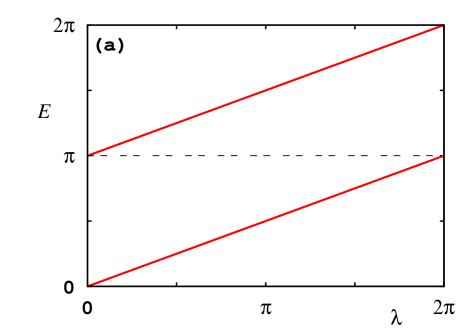
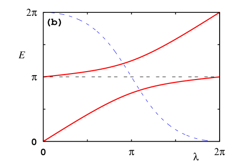
Figure 1: (Color online) Parametric motions of quasienergies (bold lines) of two-level systems. We choose the model whose “ground” quasienergy is zero at $\lambda=0$. The other quasienergy $\delta=\pi$ at $\lambda=0$ is indicated by the broken, horizontal lines. (a) The example examined in the main text, Eq. (21) ($|{}v{}\rangle=(|{}\uparrow{}\rangle-i|{}\downarrow{}\rangle)/\sqrt{2}$). The quasienergies draw two parallel lines, which have no avoided crossing. (b) A generic example ($|{}v{}\rangle=\cos(\pi/8)|{}\uparrow{}\rangle+\sin(\pi/8)|{}\downarrow{}\rangle$). There is a single avoided crossing. The broken curve represents $|\langle{}\uparrow{}|{}\xi_{0}(\lambda){}\rangle|^{2}$, which depicts that $|{}\xi_{0}(\lambda){}\rangle$ becomes orthogonal to $|{}\xi_{0}(0){}\rangle$ in the limit $\lambda\uparrow 2\pi$.

We suggest a possible implementation of the example above in a charged particle with a spin-$1/2$. Assume that the particle is localized to some place so that we may ignore the motion of the particle. The unperturbed system is the spin under a static magnetic field. The perturbation $\hat{V}$ is composed of two ingredients: One is a periodically pulsed magnetic field, whose direction needs to be different from that of the unperturbed magnetic field. The other is a periodically pulsed electric field, which provides “the constant part” of $\hat{V}$. In order to prepare $\hat{V}$, we need to adjust the ratio of the strength and the period of the two perturbation fields.

Finally, we show another example that involves multiple levels in Fig. 2 (a), where all quasienergies are involved in the anholonomy. This is due to the cyclicity of $|{}v{}\rangle$. In Fig. 2 (b), we also show an example that breaks the cyclicity of $|{}v{}\rangle$. This suggests that we may control the anholonomy to the limited number of states by an appropriate choice of $|{}v{}\rangle$.

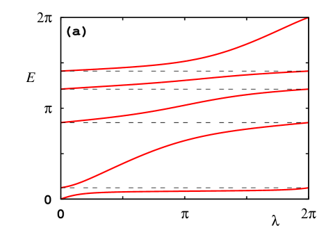
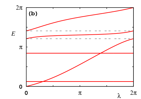
Figure 2: (Color online) Parametric motions of quasienergies (bold lines) in systems with multiple levels ($\dim\mathcal{H}=5$). The unperturbed Floquet operator $\hat{U}_{0}$, whose “ground” quasienergy is adjusted to zero at $\lambda=0$, is randomly chosen. The quasienergies at $\lambda=0$ are indicated by the broken, horizontal lines. (a) A random choice of $|{}v{}\rangle$, which satisfies cyclicity for $\hat{U}_{0}$. All quasienergies exhibit anholonomy. (b) An example for broken cyclicity in $|{}v{}\rangle$: Only three components of $|{}v{}\rangle$, in the representation that diagonalizes $\hat{U}_{0}$, take nonzero values. The resultant parametric changes and anholonomy occur only in the subspace ${\rm span}\left\{\hat{U}_{0}^{m}|{}v{}\rangle\right\}_{m}$, whose dimensionality is three. The other two quasienergies draw horizontal lines, since they correspond to the trivial eigenvectors mentioned in Section III, and are not affected by the perturbation.

VI Geometry and abundance of quasienergy anholonomy

We remark on the geometry of the quasienergy anholonomy to discuss its stability and abundance. Concerning Cheon’s eigenenergy anholonomy in a family of systems with generalized pointlike potentials, Tsutsui, Fülop, and Cheon examined the geometry of the anholonomy using the fact that the parameter space of the family is $U(2)$ Cheon:AP-294-1 ; Tsutsui:JMP-42-5687 . When the dimension of the Hilbert space is two, Tsutsui et al.’s argument is immediately applicable to the quasienergy anholonomy in the systems whose unit time evolution is described by a Floquet operator, which is a $2\times 2$ unitary matrix. We employ a parametrization of such systems by their quasienergy-spectrum $\{(E_{0},E_{1})\}$ (Fig. 3 (a)), whose element $(E_{0},E_{1})$ is identified with $(E_{1},E_{0})$. The quotient quasienergy-spectrum space is accordingly an orbifold $T^{2}/\mathbb{Z}_{2}$ which has two topologically inequivalent and nontrivial cycles (see Fig. 3 (c) and Ref. Tsutsui:JMP-42-5687 ). One cycle traverses the degeneracy line $E_{0}=E_{1}$. The other cycle concerns the “increment” (or “decrement”) of the quantum number. More precisely, the winding number along the latter cycle determines the increment of the quantum number (Fig. 3 (d)). When the dimension of Hilbert space is larger than 2, similar geometrical argument will be possible. The geometrical nature implies that the quasienergy anholonomy is stable against perturbations that preserves the topology of the cycle. Hence we may expect that the same anholonomy appears in nonautonomous systems whose unit time evolution is described by a Floquet operator, e.g., periodically kicked systems and periodically driven systems.

The stability of Cheon’s anholonomies against perturbations is also expected from the fact that the parametric dependence of the quasienergies has no crossings (see Figs. 1 and 2 (a)). To achieve the stability in practice, the gap of narrowly avoided crossings needs to be enlarged. This is possible with a suitable adjustment of $|{}v{}\rangle$ (e.g., see Figs. 1 (a) and (b)). We also remark that the presence of the trivial eigenvectors, which are introduced in Section III, induces the crossings of quasienergies, as can be seen in Fig. 2 (b) and in Appendix A. Hence quasienergy anholonomies coexisting with trivial eigenvectors are fragile against perturbations in general.

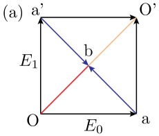
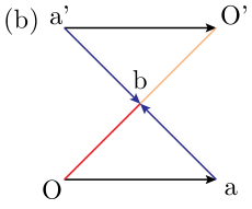
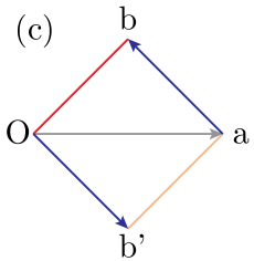
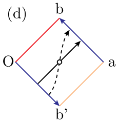
Figure 3: (Color online) A parametrization with the quasienergy-spectrum of quantum systems whose unit time evolutions are described by two-dimensional Floquet operators is explained. (a) An $E_{0}-E_{1}$ plane, where a and a’ are at $(0,2\pi/T)$ and $(2\pi/T,0)$, respectively. Because of the periodicity of quasienergies, pairs of lines Oa and a’O’, and, Oa’ and aO’ are identified. On the diagonal line $E_{0}=E_{1}$, two quasienergies are degenerate. In the subsequent figures, $(E_{0},E_{1})$ and $(E_{1},E_{0})$ are identified. (b) $\triangle$Oba’ and $\triangle$O’ba are identified with $\triangle$Oba and $\triangle$O’ba’, respectively, and so are removed. (c) The quotient space $T^{2}/\mathbb{Z}_{2}$. Since Oa and a’O’ in (b) are identical, they are arranged to make a square. Furthermore, if identical lines Ob’ and ab are put together, a Möbius strip with edges Ob and ab’, which are degenerate lines, is obtained (see Ref. Tsutsui:JMP-42-5687 ). (d) Parametric motion of spectrum on $T^{2}/\mathbb{Z}_{2}$. Bold and dashed lines, which are topologically equivalent on the Möbius strip, correspond to Figs. 1 (a) and (b), respectively, where $T=1$ is assumed. At $\lambda=0$, they start from the open circle at $(0,\pi)$. As $\lambda$ increases, they move toward ab. At $\lambda=\pi$, they arrive on a point on a line ab, which is identical with $Ob^{\prime}$. Then they return to $(0,\pi)$. Such a winding along the Möbius strip induces the quasienergy anholonomy.

VII Application: anholonomic quantum state manipulation

As an application of the quasienergy anholonomy, a design principle of systems that achieve manipulations of quantum states with adiabatic passages is proposed. Before describing our argument, we mention that the conventional works on the application of adiabatic passages to the manipulation of quantum states are the textbook results QuantumControlTexts . At the same time, there are interesting proposals on quantum circuits whose elementary operations are composed by adiabatic processes AdiabaticControl . The reason why the adiabatic processes are employed is that the operations governed by the adiabatic processes are expected to be stable. On the other hand, the manipulation that involves the phase anholonomy is expected to be stable under the perturbation, due to its topological nature.

Our scheme proposed here also relies on the adiabatic processes and employs nonconventional, Cheon’s anholonomies in quantum maps. The aim is to evolve a quantum state (“the initial target”) into another state (“the final target”). What we need to carry it out is twofold: One is an “unperturbed” Hamiltonian $\hat{H}_{0}$, whose eigenstates must contain the two target states. The other is a normalized vector $|{}v{}\rangle$, which must have nonzero overlappings between the two target states. Under the influence of a periodically pulsed perturbation $\hat{V}=|{}v{}\rangle\langle{}v{}|$ with its period $T$ and strength $\lambda$, the system is described by the kicked Hamiltonian $\hat{H}(t)$ (1). The use of the quasienergy anholonomy of the corresponding Floquet operator $\hat{U}_{\lambda}$ (2) is straightforward if $\hat{H}_{0}$ is bounded and contains only discrete eigenenergies and $T$ is smaller than $2\pi\hbar/W$, where $W$ is the difference between the maximum and the minimum eigenenergies of $\hat{H}_{0}$. Otherwise, we need to achieve these conditions effectively, by adjusting $|{}v{}\rangle$. For example, $|{}v{}\rangle$ needs to be prepared to have no overlapping with the eigenstates that have higher eigenergies to make an effective energy cutoff on $\hat{H}_{0}$.

Once we prepare such $\hat{U}_{\lambda}$, it is straightforward to realize the manipulation, at least, in theory. To convert a state vector, which is initially in an eigenstate of $\hat{U}_{0}$, to the nearest higher eigenstate of $\hat{U}_{0}$, is achieved by applying the periodically pulsed perturbation $\hat{V}=|{}v{}\rangle\langle{}v{}|$, whose strength $\lambda$ is adiabatically increased from 0 to $2\pi$. Note that at the final stage of the manipulation, we may switch off the perturbation suddenly, due to the periodicity of the Floquet operator $\hat{U}_{2\pi}=\hat{U}_{0}$. This closes a “cycle.” By repeating the cycle, the final state can be any eigenstate of $\hat{U}_{0}$. Note that, along the operation, $|{}v{}\rangle$ may vary adiabatically. In other words, the adiabatically slow fluctuation on $|{}v{}\rangle$ does no harm. We remark that an application of the present procedure to anholonomic adiabatic quantum computation is described in a separate publication TM061 .

The strongest limitations of the present scheme, in our opinion, is that the target states for the manipulation must be eigenstates of $\hat{H}_{0}$. Superpositions of the eigenstates of $\hat{H}_{0}$ cannot be the targets due to the presence of dynamical phases that generally diverge in adiabatic processes. Note that, however, there is no obstacle to handle “superposed states” when they are eigenstates of $\hat{H}_{0}$. Furthermore, if we could introduce Cheon’s anholonomies to the systems whose quasienergy are degenerate, it may be possible to carry out a coherent manipulation within a degenerate eigenspace. This motivates us to seek an extension of the eigenspace anholonomy for degenerate eigenspace, i.e., Cheon’s anholonomies á la Wilczek and Zee.

VIII Discussion and summary

We have discussed Cheon’s anholonomies in a family of quantum map (9) with a rank-one projection $\hat{V}$. Although our geometrical argument in Section VI assures the abundance of the systems that exhibit the anholonomies, we still do not have any systematic way to find such systems, except the quantum map (9). In order to suggest exploring other examples of the anholonomies, we summarize conditions to find the anholonomies. Two ingredients in our Floquet operator (9) facilitate us to find the anholonomies: (a) the periodicity of the Floquet operator for the parameter $\lambda$ enforces the periodicity of the spectrum; and (b) the positivity of the perturbation assures the monotonic increment of each quasienergy for the increment of $\lambda$. These two facts imply that $E_{n}(\lambda)$ arrives at a higher excited quasienergy $E_{n+\delta n}(\lambda)$ ($\delta n>0$) after an increment of $\lambda$ by the period $2\pi$. To realize the first condition, $\hat{V}$ needs not to be a projection operator. For the Floquet operator (2), the condition for the periodicity is $e^{-i\Lambda\hat{V}/\hbar}=1$, where $\Lambda$ is the period. In terms of the eigenvalues $\left\{v_{n}\right\}_{n}$ of $\hat{V}$, this condition is that $\Lambda v_{n}/(2\pi\hbar)$ is an integer for all $n$. Although we suppose that the anholonomies may be realized without the condition (b), we are not aware of any examples, except the trivial cases, e.g., $\hat{V}$ is negative definite. Furthermore, the above two conditions generally do not determine the exact value of $\delta n$, which is the increment of the quantum number after a single cycle, whereas $\delta n=1$ for a rank-1 projection $\hat{V}$ is shown in Section IV. The value of $\delta n$ could be determined by the geometric argument shown in Section VI. However, no systematic algorithm to compute $\delta n$ from a given family of Floquet operators is known to us.

Appendix A A reduction of Hilbert space for a quantum map under a rank-$1$ perturbation

We explain a procedure to reduce the Hilbert space for the quantum map under a rank-$1$ perturbation (9). Let us start from $\lambda=\lambda_{0}$. Assume that $\hat{U}_{\lambda_{0}}$ has a pure point spectrum (i.e., the eigenvectors of $\hat{U}_{\lambda}$ form a complete orthogonal system) KatoPurePoint . We exclude the case that $|{}v{}\rangle$ is an eigenvector of $\hat{U}_{\lambda_{0}}$ because this implies that the whole Hilbert space becomes trivial, as is explained in Section III. An eigenspace $\mathcal{H}_{z}$ of $\hat{U}_{\lambda_{0}}$, where $z$ is the corresponding eigenvalue, is reduced as follows. First, we introduce $\mathcal{H}_{z}^{\rm n}$, which is a subspace of $\mathcal{H}_{z}$ and orthogonal to $|{}v{}\rangle$:

$$\mathcal{H}_{z}^{\rm n}\equiv{\rm span}\left\{|{}\xi{}\rangle\in\mathcal{H}_{z};\langle{}v{}|{}\xi{}\rangle=0\right\}.$$ (24)

We exclude $\mathcal{H}_{z}^{\rm n}$, since this is a trivial eigenspace of $\hat{U}_{\lambda}$ (see Eq. (10)). If the remainder $\mathcal{H}_{z}^{\rm p}\equiv\mathcal{H}_{z}\ominus\mathcal{H}_{z}^{\rm n}$ is not $\left\{0\right\}$, $\mathcal{H}_{z}^{\rm p}$ is a one-dimensional eigenspace of $\hat{U}_{\lambda_{0}}$. Hence the degeneracy in the eigenvalue $z$ is removed. Then we examine the spectrum of $\hat{U}_{\lambda}$ on the resultant Hilbert space $\mathcal{H}\equiv\oplus_{z}\mathcal{H}_{z}^{\rm p}$. On $\mathcal{H}$, $\hat{U}_{\lambda_{0}}$ has a pure point and nondegenerate spectrum. At the same time, all of the eigenvector $|{}\xi{}\rangle$ of $\hat{U}_{\lambda_{0}}$ satisfies

$$0\lvertneqq|\langle{}v{}|{}\xi{}\rangle|\lvertneqq 1.$$ (25)

For general $\lambda$, we assume that $\hat{U}_{\lambda}$ also has a pure point spectrum. Namely, we exclude the case that $\hat{U}_{\lambda}$ has a continuous spectrum, which emerges under some combinations of $\hat{U}_{\lambda_{0}}$ and $|{}v{}\rangle$ in an infinite dimensional $\mathcal{H}$ Combescure:JSP-59-679 . As a result of the reduction of $\mathcal{H}$, any eigenvector $|{}\xi{}\rangle$ of $\hat{U}_{\lambda}$ also satisfies the inequality (25). Hence we proved the inequality (12) in the main text.

Appendix B Cyclicity

When a Hilbert space $\overline{{\rm span}\{\hat{U}^{m}|{}v{}\rangle\}_{m=0}^{\infty}}$, which is induced by a vector $|{}v{}\rangle$ and an operator $\hat{U}$, agrees with the whole Hilbert space, $|{}v{}\rangle$ is called a cyclic vector of $\hat{U}$ RSICyclicity . The notion of the cyclicity is useful to discuss how we choose $|{}v{}\rangle$ in the quantum map (9) to find Cheon’s anholonomies, as is explained in Sections III to V. Hence a review of the cyclicity is shown below, where we assume that the spectrum of $\hat{U}$ has only discrete and finite components.

A characterization of the cyclic vector $|{}v{}\rangle$ for $\hat{U}$ is explained: Any (normalizable) eigenvector $|{}\xi{}\rangle$ of $\hat{U}$ satisfies $\langle{}\xi{}|{}v{}\rangle\neq 0$. To show this, let $z$ be the eigenvalue corresponding to $|{}\xi{}\rangle$. Due to the cyclicity, $|{}\xi{}\rangle$ is a linear combination of $\{\hat{U}^{m}|{}v{}\rangle\}_{m=0}^{\infty}$, i.e., $|{}\xi{}\rangle=\sum_{m=0}^{\infty}c_{m}\hat{U}^{m}|{}v{}\rangle$ with appropriate coefficients $c_{m}$. Hence we have $\langle{}\xi{}|{}\xi{}\rangle=\sum_{m=0}^{\infty}c_{m}\langle{}\xi{}|\hat{U}^{m}|{}v{}\rangle=\sum_{m=0}^{\infty}c_{m}z^{m}\langle{}\xi{}|{}v{}\rangle=\left(\sum_{m=0}^{\infty}c_{m}z^{m}\right)\langle{}\xi{}|{}v{}\rangle$. Since $\langle{}\xi{}|{}\xi{}\rangle$ is nonzero and $\sum_{m=0}^{\infty}c_{m}z^{m}$ is finite, we conclude $\langle{}\xi{}|{}v{}\rangle\neq 0$. Note that this just proves the fact that the condition (ii’) implies the condition (ii) in Section III.

Next, we show that the inverse holds, i.e., the condition (ii) implies the condition (ii’) when the spectrum of $\hat{U}$ is nondegenerate. More precisely, when all eigenvectors $|{}\xi{}\rangle$ of $\hat{U}$ satisfy $\langle{}v{}|{}\xi{}\rangle\neq 0$, $|{}v{}\rangle$ is a cyclic vector for $\hat{U}$. To show this, we prove that $\left\{\hat{U}^{m}|{}v{}\rangle\right\}_{m=0}^{N-1}$ are linearly independent, where $N$ is the number of the eigenvalues. Namely, for an $N$-dimensional vector $\boldsymbol{c}=(c_{0},c_{1},\ldots,c_{N-1})$, we show that

$$\sum_{m=0}^{N-1}c_{m}\hat{U}^{m}|{}v{}\rangle=0$$ (26)

implies $\boldsymbol{c}=0$. Let $z_{n}$ and $|{}\xi_{n}{}\rangle$ denote an eigenvalue of $\hat{U}$ and the corresponding eigenvector, respectively ($n=0,1,\ldots,N-1$). From Eq. (26), we have $\sum_{m=0}^{N-1}\langle{}\xi_{n}{}|{}\hat{U}^{m}{}|{}v{}\rangle c_{m}=\langle{}\xi_{n}{}|{}v{}\rangle\sum_{m=0}^{N-1}(z_{n})^{m}c_{m}=0.$ The assumption $\langle{}\xi_{n}{}|{}v{}\rangle\neq 0$ implies $\sum_{m=0}^{N-1}(z_{n})^{m}c_{m}=0$ for all $n$. This is written as $A\boldsymbol{c}=0$, where $A$ is the $N$-dimensional square matrix whose $(m,n)$-element is $(z_{n})^{m}$. Accordingly we encounter a Vandermonde determinant

$$\det A =\begin{vmatrix}1&z_{0}&(z_{0})^{2}&\dots&(z_{0})^{N-1}\\ 1&z_{1}&(z_{1})^{2}&\dots&(z_{1})^{N-1}\\ {5}\\ 1&z_{N-1}&(z_{N-1})^{2}&\dots&(z_{N-1})^{N-1}\end{vmatrix}$$

$$=\prod_{n^{\prime\prime}>n^{\prime}}(z_{n^{\prime\prime}}-z_{n^{\prime}})$$ (27)

and we have $\det A\neq 0$ due to the absence of spectrum degeneracy of $\hat{U}$. Hence we have $\boldsymbol{c}=0$.

We can now examine the condition when $\hat{U}$ has a cyclic vector to see the correspondence between the conditions (i) and (i’) in Section III. If the spectrum of $\hat{U}$ is nondegenerate, $\hat{U}$ has a cyclic vector, e.g., $\sum_{n=0}^{N-1}|{}\xi_{n}{}\rangle$, from the above discussion. Furthermore, $\hat{U}$ has a cyclic vector only when $\hat{U}$ has no degenerate eigenvalue. To show the latter, we examine its contraposition. Hence we assume that $\hat{U}$ has a degenerate eigenvalue, i.e., $\det A=0$. Accordingly we have a nonzero $\boldsymbol{c}$ that satisfies $A\boldsymbol{c}=\boldsymbol{0}$, i.e., $\sum_{m=0}^{N-1}(z_{n})^{m}c_{m}=0$ for all $n$. With such $\boldsymbol{c}$ and arbitrary $d_{n}$, we have $0=\sum_{n=0}^{N-1}d_{n}\langle{}\xi_{n}{}|\sum_{m=0}^{N-1}(z_{n})^{m}c_{m}=\sum_{n=0}^{N-1}d_{n}\langle{}\xi_{n}{}|\sum_{m=0}^{N-1}\hat{U}^{m}c_{m},$ i.e., $\sum_{m=0}^{N-1}c_{m}\hat{U}^{m}=0$. Accordingly, with any vector $|{}v{}\rangle$, we have $\sum_{m=0}^{N-1}c_{m}\hat{U}^{m}|{}v{}\rangle=0$, i.e., $\left\{\hat{U}^{m}|{}v{}\rangle\right\}_{m=0}^{N-1}$ is linearly dependent and any $|{}v{}\rangle$ cannot be a cyclic vector for $\hat{U}$. Thus the degenerate eigenvalue of $\hat{U}$ leads to an absence of its cyclic vector.

To summarize this appendix, we explain the conditions (i’) and (ii’) in Section III. If the spectrum of $\hat{U}$ is finite and nondegenerate, $\hat{U}$ has a cyclic vector. Furthermore, if $|{}v{}\rangle$ satisfies $\langle{}v{}|{}\xi{}\rangle\neq 0$ for any eigenvector $|{}\xi{}\rangle$ of $\hat{U}$, $|{}v{}\rangle$ is a cyclic vector of $\hat{U}$.

References

- (1) A. Shapere and F. Wilczek, eds., Geometric phases in physics (World Scientific, Singapore, 1989); A. Bohm, A. Mostafazadeh, H. Koizumi, Q. Niu, and Z. Zwanziger, The Geometric Phase in Quantum Systems (Springer, Berlin, 2003).
- (2) M. V. Berry, Proc. Roy. Soc. London A 430, 405 (1984).
- (3) M. Born and V. Fock, Z. Phys 51, 165 (1928).
- (4) F. Wilczek and A. Zee, Phys. Rev. Lett. 52, 2111 (1984).
- (5) T. Cheon, Phys. Lett. A 248, 285 (1998).
- (6) T. Cheon, T. Fülöp, and I. Tsutsui, Ann. Phys. (NY) 294, 1 (2001).
- (7) I. Tsutsui, T. Fülöp, and T. Cheon, J. Math. Phys. 42, 5687 (2001).
- (8) M. Born and R. Oppenheimer, Ann. Phys. (Leipzig) 84, 457 (1927).
- (9) M. Born and K. Huang, Dynamical Theory of Crystal Lattices (Clarendon Press, Oxford, 1954).
- (10) C. Kittel, Introduction to solid state physics (John Wiley & Sons, New York, 1953).
- (11) I. Tsutsui, T. Fülöp, and T. Cheon, J. Phys. A. 36, 275 (2003).
- (12) H.-J. Stöckmann, Quantum Chaos (Cambridge University Press, Cambridge, 1999), Chap. 4.
- (13) A. Tanaka and M. Miyamoto, Phys. Rev. Lett. 98, 160407 (2007).
- (14) For example, in the systems which have infinite dimensional Hilbert space, it is possible that may have a continuous spectrum under the presence of a perturbation Combescure:JSP-59-679 and the parametric motion of eigenvalue may have indifferentiability [D. W. Hone, R. Ketzmerick, and W. Kohn, Phys. Rev. A 56, 4045 (1997)].
- (15) M. Combescure, J. Stat. Phys. 59, 679 (1990).
- (16) K. Nakamura and H. J. Mikeska, Phys. Rev. A 35, 5294 (1987).
- (17) C. Mead and D. G. Truhlar, J. Chem. Phys. 70, 2284 (1979).
- (18) More precisely, we need a set of equations for to obtain a complete set of the equations of motion Nakamura:PRA-35-5294 .
- (19) M. Holthaus, Phys. Rev. Lett. 69, 1596 (1992).
- (20) M. Reed and B. Simon, Methods of modern mathematical physics I: Functional analysis (Academic Press, San Diego, 1980), chap. VII, revised and enlarged ed.
- (21) Since we assume that the dimensionality of the whole Hilbert space is finite (say, ), is linearly dependent. We may use an exact truncation in the condition of the cyclicity.
- (22) S. A. Rice and M. Zhao, Optical control of molecular dynamics (John Wiley and Sons, inc., 2000); M. Shapiro and P. Brumer, Principles of the Quantum Control of Molecular Processes (Wiley, New York, 2003).
- (23) P. Zanardi and M. Rasetti, Phys. Lett. A 264, 94 (1999); J. A. Jones, V. Vedral, A. Ekert, and G. Castagnoli, Nature 403, 869 (2000); E. Farhi, J. Goldstone, S. Gutmann, and M. Sipser (2000), eprint quant-ph/0001106.
- (24) T. Kato, Perturbation Theory for Linear Operators (Springer-Verlag, Berlin, 1980), chap. X, corrected printing of the second ed.