Many body generalization of the Landau Zener problem

Abstract

We formulate and approximately solve a specific many-body generalization of the Landau-Zener problem. Unlike with the single particle Landau-Zener problem, our system does not abide in the adiabatic ground state, even at very slow driving rates. The structure of the theory suggests that this finding reflects a more general phenomenon in the physics of adiabatically driven many particle systems. Our solution can be used to understand, for example, the behavior of two-level systems coupled to an electromagnetic field, as realized in cavity QED experiments.

The Landau-Zener (LZ) problem describes a paradigmatic situation in physics where two quantum levels cross each other in time. In its most basic form, the problem is represented by the Hamiltonian

$$H=\left(\matrix{\lambda t&g\cr g&-\lambda t}\right),$$ (1)

where $t$ is time, $g$ the coupling constant, and $\lambda$ the rate of change of the energy levels (here, as in the rest of the paper, we set $\hbar=1$). This Hamiltonian has two instantaneous energy levels $E_{\pm}=\pm\sqrt{(\lambda t)^{2}+g^{2}}$. Suppose in the distant past, $t\rightarrow-\infty$, the system is in level $E_{-}$. The goal then is to calculate the probability, $P$, to stay in $E_{-}$ at $t\rightarrow+\infty$. Solving the corresponding time dependent Schrödinger equation, Landau  Landau (1932) and Zener Zener (1932) found

$$P=1-e^{-\frac{\pi g^{2}}{\lambda}},$$ (2)

as an exact answer to this question: if only the sweeping rate is slow enough, it is exponentially likely that the system will abide in its adiabatic ground state. For 75 years, the Hamiltonian (1), and its solution (2) have been used to describe a huge spectrum of physical phenomena Landau and Lifshitz (1981). Subsequent generalizations of (1) include an extension to a multi-channel environment wherein the 2 by 2 matrix is replaced by a larger time-dependent matrix. However, common to all those problems Demkov (1966); Osherov (1966); Kayanuma and Fukichi (1985); Brundobler and Elser (1993) is that only a finite number of degrees of freedom participate in the transition process (which manifests itself in transition probabilities of the same algebraic structure as in Eq. (2).)

At the same time, there appears to be some interest in genuine fn_ many-body generalizations of the LZ setup: fundamentally, one would like to know whether a slowly driven many body system will remain in its adiabatic ground state, in a manner resembling the single particle case (2). But there is also applied relevance to the generalization. A number of existing experimental setups provide a perspective to actually probe the transition rates of a many-body LZ problem. Examples include systems of $N$ two-level systems (’atoms’, either real or artificial), coupled to a photon mode in a cavity Kaluzny et al. (1983); Wallraff et al. (2004). In this case, time dependence might be introduced by changes of either the photon frequency (by changing the cavity’s size), or the energy splitting of the two level systems (by applying a ’Zeeman’ field.) Similar physics also arises in the context of polaritons, excitons coupled to a cavity electromagnetic mode Weisbuch et al. (1992). Another phenomenon relevant to the present work is the observation of molecule production in an atomic gas experiment, due to sweeping through a Feshbach resonance Regal et al. (2004); Zwierlein et al. (2004). While the fast sweep regime was analyzed in Refs. Altman and Vishwanath (2005); Barankov and Levitov (2005), the complementary case of slow sweeping rates, equivalent to a many-body LZ problem Dobrescu and Pokrovsky (2006); Tikhonenkov et al. (2006), has not yet been understood.

Having the above setup of two level systems coupled to a cavity mode in mind, we consider the Hamiltonian

$$H=-\lambda t~{}\hat{b}^{\dagger}\hat{b}+\frac{\lambda t}{2}\sum_{i=1}^{N}\sigma^{z}_{i}+\frac{g}{\sqrt{N}}\sum_{i=1}^{N}\left(\hat{b}^{\dagger}\,\sigma^{-}_{i}+\hat{b}\,\sigma^{+}_{i}\right),$$ (3)

where $\hat{b}^{\dagger}$ creates a photon mode, and $\sigma^{\pm}_{i}$ are raising and lowering operators of the $i-$th two level system. ($\sigma^{\pm}\equiv(\sigma^{x}\pm i\sigma^{y})/2$, where $\sigma^{x,y,z}$ are Pauli matrices.) The energy of the photon and the two-level system vary in time as $\pm\lambda t$, respectively. The Hamiltonian (3) is equivalent, up to a gauge transformation, to $H=-2\lambda t~{}\hat{b}^{\dagger}\hat{b}+\omega_{0}\sum_{i=1}^{N}\sigma^{z}_{i}+\frac{g}{\sqrt{N}}\sum_{i=1}^{N}\left(\hat{b}^{\dagger}\,\sigma^{-}_{i}+\hat{b}\,\sigma^{+}_{i}\right)$, which represents a generalization of the James-Cumming Hamiltonian Jaynes and Cummings (1963) to $N$ two-level systems. Equivalently, we can think of (3) as an effective Hamiltonian describing a Feshbach resonance scenario: representing the spin operators in (3) in terms of Anderson pseudospin operators,

$$\sigma^{z}_{i}\rightarrow\hat{a}^{\dagger}_{i\uparrow}\hat{a}_{i\uparrow}-\hat{a}_{i\downarrow}\hat{a}^{\dagger}_{i\downarrow},\,\sigma^{+}_{i}\rightarrow\hat{a}^{\dagger}_{i\uparrow}\hat{a}^{\dagger}_{i\downarrow},\,\sigma^{-}_{i}\rightarrow\hat{a}_{i\downarrow}\hat{a}_{i\uparrow}$$ (4)

where $\hat{a}^{\dagger}_{i\uparrow}$, $\hat{a}^{\dagger}_{i\downarrow}$, $\hat{a}_{i\uparrow}$, $\hat{a}_{i\downarrow}$ are the creation and annihilation operator for the spin-$1/2$ fermions labeled by $i$, Eq. (3) assumes the form (up to an unimportant constant)

$$H=-\lambda t~{}\hat{b}^{\dagger}\hat{b}+\frac{\lambda t}{2}\sum_{i=1}^{N}\left(\hat{a}^{\dagger}_{i\uparrow}\hat{a}_{i\uparrow}+\hat{a}^{\dagger}_{i\downarrow}\hat{a}_{i\downarrow}\right)+$$ (5)

$$+\frac{g}{\sqrt{N}}\sum_{i=1}^{N}\left(\hat{b}^{\dagger}\,\hat{a}_{i\downarrow}\hat{a}_{i\uparrow}+\hat{b}\,\hat{a}^{\dagger}_{i\uparrow}\hat{a}^{\dagger}_{i\downarrow}\right).$$ (6)

This is nothing but the Hamiltonian describing the creation of molecules out of $N$ fermion pairs in a Feshbach resonance experiment Dobrescu and Pokrovsky (2006); Barankov and Levitov (2005) (although the single mode approximation, i.e. the neglect of bosonic dispersion, may be problematic in that case).

Assuming that the boson level is initially empty, and all fermions resident in the upper state (on account of the energy balance at large negative times),

$$\langle\,\hat{b}^{\dagger}\hat{b}\,\rangle=0,\qquad\langle\,\sigma^{z}_{i}\,\rangle=1,\;\;i=1,\dots,N,$$ (7)

our goal is to compute the asymptotic distribution

$$n_{b}(t)=\langle\,\hat{b}^{\dagger}(t)\hat{b}(t)\,\rangle$$ (8)

at $t\rightarrow\infty$, i.e. the generalization of the LZ transition probability $P$. For $N=1$, this task is equivalent to the standard LZ problem, whose answer is given by (cf. Eq. (2)) $\lim_{t\rightarrow\infty}n_{b}(t)=1-e^{-\frac{\pi g^{2}}{\lambda}}$. However, for $N>1$, Eq. (3) defines a genuine many-body problem and the solution of the corresponding Schrödinger equation becomes progressively more difficult.

While we do not know how to handle the problem for arbitrary $N$, an approximate solution valid in the limit of large particle numbers can be found. At large $N$, the number of produced bosons turns out to be reasonably well approximated by

$$\lim_{t\rightarrow\infty}n_{b}(t)= e^{\frac{\pi g^{2}}{\lambda}}-1, \qquad e^{\frac{\pi g^{2}}{\lambda}}\ll N,$$ (9)

$$\lim_{t\rightarrow\infty}n_{b}(t)\sim \frac{e^{\frac{\pi g^{2}}{\lambda}}}{\frac{2}{N}e^{\frac{\pi g^{2}}{\lambda}}+1}, \qquad e^{\frac{\pi g^{2}}{\lambda}}\sim N,$$ (10)

$$\lim_{t\rightarrow\infty}n_{b}(t)\rightarrow N, \qquad e^{\frac{\pi g^{2}}{\lambda}}\gg N.$$ (11)

According to these equations, the adiabatic ground state ($n_{b}\stackrel{{\scriptstyle t\to\infty}}{{\longrightarrow}}N$) is only realized if $\lambda\ll\pi g^{2}/\log(N)$, a criterion which is progressively more difficult to satisfy as $N$ becomes larger (see Ref. Polkovnikov and Gritsev for a general discussion of the applicability of the adiabatic limit in large systems). This is in marked contrast to the few body case, where adiabatic ground state occupancy is granted for large values of the LZ parameter $e^{\frac{\pi g^{2}}{\lambda}}$. The observation of this difference, obtained for a specific model but likely indicative of a more general phenomenon, represents the main result of the paper.

Technically, Eqs. (9) and Eq. (10) obtain by integration of a rate equation for the boson occupation number. Denoting the occupation of individual fermion states by $n_{f}$, the latter reads

$$\partial_{t}n_{b}=2\pi g^{2}\delta(2\lambda t)\left(n_{f}^{2}\left(1+n_{b}\right)-n_{b}\left(1-n_{f}\right)^{2}\right),$$

$$n_{b}+Nn_{f}=N,$$ (12)

where the factor $\delta(2\lambda t)$ accounts the energy balance in particle conversion processes, the first (second) term on the right hand side describes the creation (destruction) of bosonic particles by destruction (creation) of two fermions, and the second line enforces particle number conservation. Postponing the derivation of Eq. (Many body generalization of the Landau Zener problem), and the discussion of its range of validity to below, we note that upon introduction of a variable $\theta$, such that $\theta^{\prime}(t)=\delta(t)$, Eq. (Many body generalization of the Landau Zener problem) assumes the form

$$\partial_{\theta}n_{b}=\frac{\pi g^{2}}{\lambda}\left(n_{f}^{2}\left(1+n_{b}\right)-n_{b}\left(1-n_{f}\right)^{2}\right).$$ (13)

At $\theta=1$ (which corresponds to $t\rightarrow\infty$) the solution of this equation (with boundary condition $n_{b}=0$ at $\theta=0$) reads

$$n_{b}=\frac{N\left(e^{\frac{\pi g^{2}}{\lambda}}-1\right)}{2e^{\frac{\pi g^{2}}{\lambda}}+N},$$ (14)

where terms of $\mathcal{O}(N^{-1})$ have been ignored. Taking the limit $N\rightarrow\infty$ at fixed $e^{\pi g^{2}/\lambda}$ gives Eq. (9), while $e^{\pi g^{2}/\lambda}\sim N$ leads to Eq. (10). Although that latter limit is beyond the scope of the large $N$ expansion, (10) turns out to provide a reasonable (if uncontrolled) approximation to $n_{b}$.

To actually derive Eq. (Many body generalization of the Landau Zener problem), we apply the Keldysh formalism. Defining $t\equiv(t_{1}+t_{2})/2$ and $\tau\equiv t_{1}-t_{2}$, we denote by $G^{R,A,K}(t_{1},t_{2})\equiv G^{R,A,K}(t,\tau)$ the retarded, advanced, and Keldysh fermionic propagators, respectively. (For the general definition of Keldysh Green functions and notation conventions we refer to the review Kamenev (2005).) Initially all the $N$ fermionic levels are occupied; this corresponds to the bare (noninteracting) propagators

$$G^{R,A}_{0}(t,\tau)=\mp i\theta(\pm\tau)e^{-i\frac{\lambda}{2}t\tau},\ G^{K}_{0}(t,\tau)=ie^{-i\frac{\lambda}{2}t\tau},$$ (15)

where the upper or lower sign in $\pm$ and $\mp$ are chosen for retarded and advanced propagators respectively. We aim to compute the boson’s Keldysh propagator $D^{K}(t,\tau)$ which, when evaluated at $t=+\infty$, gives the number of produced bosons. Initially, however, the boson level was unoccupied. Thus

$$D^{R,A}_{0}(t,\tau)=\mp\theta(\pm\tau)e^{i\lambda t\tau},\ D^{K}_{0}(t,\tau)=-ie^{i\lambda t\tau}.$$ (16)

If the self energy $\Sigma(t,\tau)$ of the bosons is known, the Keldysh bosonic propagator can be found by solving the Dyson equation, $(D_{0}^{-1}-\Sigma)\circ D=\openone$ where $D_{0}\,(D)$ is the bare (dressed) bosonic propagator. Introducing the bosonic distribution matrix $F(t,t^{\prime})$ through Kamenev (2005) $D^{K}=D^{R}\circ F-F\circ D^{A}$, where $(A\circ B)(t_{1},t_{2})\equiv\int_{-\infty}^{\infty}dt_{3}\,A(t_{1},t_{3})B(t_{3},t_{2})$, and $D^{R,A,K}$ are the retarded, advanced and Keldysh components of $D$, the Dyson equation for $D^{K}$ translates to a kinetic equation

$$\left[F\stackrel{{\scriptstyle\circ}}{{,}}i\partial_{t}+\lambda t\right]=\Sigma^{K}-\left(\Sigma^{R}\circ F-F\circ\Sigma^{A}\right).$$ (17)

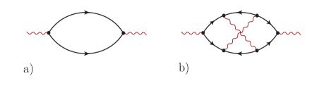
Figure 1: a) dominant self energy diagram for the bosonic propagator in the limit $N\rightarrow\infty$ with $g$ kept fixed. The straight lines are fermions, while the wavy lines are bosons. b) non-RPA diagram of lesser order in $N$.

To approximately solve this equation, we note that only interaction vertices $\sim g^{2}/N$ accompanied by one summation over $N$ fermion states survive the limit $N\to\infty$. In practice, this means that only the self energy diagram depicted in Fig. 1 a) contributes to the boson self energy. Processes such as the one shown on Fig 1 b) are frustrated in that the number of fermion summations does not compensate for the number of interaction lines. One may verify that the same logics excludes any diagram other than the one shown on Fig. 1 a). (For a caveat in the argument, see below.)

The diagram shown in Fig. 1 a) translates to

$$\Sigma^{R,A}(t,t^{\prime}) = ig^{2}\int\frac{d\omega}{2\pi}\,G^{R,A}\left(t,\epsilon-\omega\right)G^{K}\left(t,\omega\right)$$ (18)

$$\Sigma^{K}(t,t^{\prime}) = i\frac{g^{2}}{2}\sum_{k=R,A,K}\int\frac{d\omega}{2\pi}\,G^{K}\left(t,\epsilon-\omega\right)G^{K}\left(t,\omega\right).$$

on the right hand side we have switched to a Wigner representation,

$$G(t,\epsilon)\equiv\int_{-\infty}^{\infty}d\tau~{}G(t,\tau)~{}e^{i\tau\epsilon}.$$ (19)

Introducing the spectral function

$$\Delta_{f}(t,\epsilon)=2~{}{\rm Im}~{}G^{R}(t,\epsilon)$$ (20)

we obtain an equation for the Wigner transform of $F$,

$$\left(\partial_{t}-\lambda\partial_{\epsilon}\right)F(\epsilon)=\frac{g^{2}}{2}\int\frac{d\omega}{2\pi}\Delta_{f}\left(\epsilon-\omega\right)\Delta_{f}\left(\omega\right)\left[1+\right.$$ (21)

$$\left.f\left(\epsilon-\omega\right)f\left(\omega\right)-\left(f\left(\omega\right)+f\left(\epsilon-\omega\right)\right)F\left(\epsilon\right)\right].$$ (22)

Here $f(t,\epsilon)$ is the fermionic distribution function, and the argument $t$, identically carried by all Wigner functions, is suppressed for brevity. In deriving Eq. (21) we assumed that the Wigner transform of products of operators on the right hand side (e.g. $(\Sigma^{R}\circ F)(\epsilon,T)$) can be replaced by the product of the Wigner functions ($\Sigma(\epsilon,T)F(\epsilon,T)$). As discussed a few paragraphs further down, this leading adiabatic approximation Kamenev (2005) turns out to be exact in our case. Also note that Eq. (21) was derived without specifying whether the fermionic propagators in Fig. 1 a) are bare or dressed.

Noting that in the distant future fermions and bosons become effectively uncorrelated and the energy of the latter asymptotes to $\epsilon=-\lambda t$, our aim is to calculate the bosonic distribution function, $n_{b}(t)\equiv n_{b}(t,\epsilon=-\lambda t)$. To transform Eq. (21) into an equation for $n_{b}$ we use the general relations $n_{b}=(F-1)/2$, $n_{f}=(1-f)/2$, and note that $d_{t}n_{b}=(\partial_{t}-\lambda\partial_{\epsilon})F/2$. Approximating the fermion spectral functions by their bare value, $A(\epsilon)=-2\pi\delta(\epsilon-\lambda t)$, we then readily arrive at Eq. (Many body generalization of the Landau Zener problem), where all fermionic distribution functions $n_{f}(t)\equiv n_{f}(t,0)$ are evaluated at zero energy.

Let us examine the status of the various approximations used in the derivation of the rate equation: In the language of diagrammatic perturbation theory, Eq. (21) treats the bosonic and fermionic Keldysh components of the self energy operators in a self consistent RPA approximation (i.e. a scheme wherein all ’crossing’ interaction lines in the bosonic and fermionic self energy are neglected, on account of the limit $N\to\infty$.) Notice that a naive interpretation of the large $N$ limit would suggest to neglect the fermion self energy altogether: interaction corrections to the fermion propagator do not come with a final state summation and are, therefore, superficially of $\mathcal{O}(N^{-1})$. However, this argument neglects that in regimes (10) and (11) above, the bosonic distribution function $F\sim n_{b}\sim N$ introduces additional $N$ dependence into the theory. (Physically, the macroscopic occupation of the boson level effectively enhances the fermion scattering rate.) This mechanism requires us to keep the RPA self energy of the fermionic Keldysh Green function. However, the self energy corrections to the retarded and advanced fermion propagators, which are independent of the bosonic distribution function, are indeed large $N$ negligible. This latter simplification justifies the above approximation of the fermion spectral function by its bare value. (For the sake of completeness we mention the existence of non-RPA diagrams in which a nominally low power in $N^{-1}$ competes with factors $n_{b}$. [This happens, e.g., in the Keldysh sector of the diagram shown in Fig. 1 b).] These processes are not captured in our present analysis which means that the theory becomes effectively uncontrolled once $n_{b}\sim N$.)

We finally comment on the status of the leading order Moyal expansion $(\Sigma\circ F)(\epsilon,T)\simeq\Sigma(\epsilon,T)F(\epsilon,T)$ used in the derivation. The temporal singularity $\sim\delta(t)$ of the collision integral makes one worry that this replacement may, indeed, not be entirely innocent. While we cannot really justify the approximation in the resonant time window $t\sim 0$, we have checked that it does yield the correct long time asymptotics (2) when applied to the standard LZ evolution equation.

It is instructive to reconsider the derivation of Eq. (9) from a somewhat different perspective: the fact that the Hamiltonian (3) contains the Pauli matrices only in certain linear combinations enables us to attack the problem by spin algebraic methods. We define an ${\rm SU}(2)$ algebra of spin operators $\{S^{z},S^{+},S^{-}\}$ acting in an $N/2$ dimensional Hilbert space as $\hat{S}^{z}=\frac{1}{2}\sum_{i=1}^{N}\sigma^{z}_{i}$, $\hat{S}^{\pm}=\sum_{i=1}^{N}\sigma^{\pm}$. Eq. (7) enforces full initial polarization, $\langle\,\hat{S}^{z}\,\rangle=N/2$.

Since the total number of bosons produced is much less than $N$ (the defining criterion of the regime Eq. (9)), the spin will not deviate much from the vertical direction, and it is convenient to employ a Holstein-Primakoff representation: replacing Beige et al. (2005) $\hat{S}^{+}\rightarrow\sqrt{N}\,\hat{b}_{HP}$, $\hat{S}^{-}\rightarrow\sqrt{N}\,\hat{b}^{\dagger}_{HP}$, $\hat{S}^{z}=N/2-\hat{b}^{\dagger}_{HP}\hat{b}_{HP}$, where $\hat{b}_{HP}^{\dagger}$ and $\hat{b}_{HP}$ are the creation and annihilation operators of an auxiliary Holstein-Primakoff boson, the large $N$ limit of the Hamiltonian Eq. (3) reduces to the quadratic form

$$H=-\lambda t~{}\hat{b}^{\dagger}\hat{b}-\lambda t~{}\hat{b}_{HP}^{\dagger}\hat{b}_{HP}+g\left(\hat{b}^{\dagger}\,\hat{b}^{\dagger}_{HP}+\hat{b}\,\hat{b}_{HP}\right).$$ (23)

The solution of the equations of motion of (23) then leads to Eq. (9). (In a slightly different context, these equations have been solved in Kayali and Sinitsyn (2003), where Eq. (9) was derived for the first time.) However, the above method does not appear to be straightforwardly extensible to the regime of large transition rates, Eq. (10).

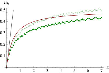
Figure 2: The boson production $n_{b}$ as a function of $x=\exp\left(\pi g^{2}/\lambda\right)/N$. Here $N=100$ (empty circles) and $N=500$ (filled circles). The straight line represents Eq. (9) and the curve is Eq. (10). The data is obtained by solving the Schrödinger equation for Eq. (3) at $g=1$, on the interval $-40\leq t\leq 40$, with the small oscillations in the data being the artifact of the finite time interval.

To check the validity of our results we have run a numerical test. The above spin representation shows that the Hilbert space of the problem is of dimension $N+1$ (much lower than the $\mathcal{O}(2^{N})$ naively suggested by the representation (3)); this makes a numerical solution of the Schrödinger equation feasible. Fig. 2 shows $n_{b}$ as a function of $x=\exp\left(\pi g^{2}/\lambda\right)/N$ for $N=100$ and $N=500$. At $N=100$ the data is in general agreement with Eqs. (9) and (10), at larger $N$ we observe gradual downward deviations. Preliminary results based on a combination of semiclassical ideas and numerical integration indeed suggest the existence of corrections in $\ln(N)$ (at fixed value $x>1$). However, in all our simulations, the fraction $n_{b}/N$ converged to values below that predicted by Eq. (10), i.e. our principal observation of incomplete ground state occupation remains valid.

To conclude, we have studied a genuine many body generalization of the Landau-Zener problem. Unlike with the single particle case, the system does not settle in its many particle ground state and a finite fraction of particles remains in energetically high-lying states. This phenomenon makes many body Landau-Zener physics profoundly different from the few body case.

V.G. is grateful to the participants of the KITP, Santa Barbara, program ’Strongly Correlated States in Condensed Matter and Atomic Physics’ and especially to R. Barankov, J. Keeling, A. Beige, V. Pokrovsky, and A. Polkovnikov for many comments and useful discussions. A.A. acknowledges discussions with A. Rosch and B. Simons. This work was supported by SFB/TR 12 of the Deutsche Forschungsgemeinschaft and by NSF via grants DMR-0449521 and PHY-0551164.

References

- Landau (1932) L. Landau, Phys. Z. Sowj. 2, 46 (1932).
- Zener (1932) C. Zener, Proc. R. Soc. 137, 696 (1932).
- Landau and Lifshitz (1981) L. D. Landau and E. M. Lifshitz, Quantum Mechanics (Butterworth-Heinemann, Oxford, UK, 1981).
- Demkov (1966) Y. N. Demkov, Sov. Phys.-Dokl. 11, 138 (1966).
- Osherov (1966) V. I. Osherov, Sov. Phys. JETP 22, 804 (1966).
- Kayanuma and Fukichi (1985) Y. Kayanuma and S. Fukichi, J. Phys. B: At. Mol. Phys. 18, 4089 (1985).
- Brundobler and Elser (1993) S. Brundobler and V. Elser, J. Phys. A: Math. Gen. 26, 1211 (1993).
- (8) I.e. generalizations that defy transformation to an (effectively single particle) quadratic Hamiltonian Kayali and Sinitsyn (2003).
- Kaluzny et al. (1983) Y. Kaluzny et al., Phys. Rev. Lett. 51, 1175 (1983).
- Wallraff et al. (2004) A. Wallraff et al., Nature 431, 162 (2004).
- Weisbuch et al. (1992) C. Weisbuch et al., Phys. Rev. Lett. 69, 3314 (1992).
- Regal et al. (2004) A. Regal, M. Greiner, and D. S. Jin, Phys. Rev. Lett. 92, 040403 (2004).
- Zwierlein et al. (2004) M. W. Zwierlein et al., Phys. Rev. Lett. 92, 120403 (2004).
- Altman and Vishwanath (2005) E. Altman and A. Vishwanath, Phys. Rev. Lett. 95, 110404 (2005).
- Barankov and Levitov (2005) R. Barankov and L. Levitov (2005), eprint cond-mat/0506323.
- Dobrescu and Pokrovsky (2006) B. E. Dobrescu and V. L. Pokrovsky, Phys. Lett. A 350, 154 (2006).
- Tikhonenkov et al. (2006) I. Tikhonenkov et al., Phys. Rev. A 73, 043605 (2006).
- Jaynes and Cummings (1963) E. T. Jaynes and F. W. Cummings, Proc. Inst. Elect. Eng. 51, 89 (1963).
- (19) A. Polkovnikov and V. Gritsev, eprint arXiv:0706.0212.
- Kamenev (2005) A. Kamenev, in Nanophysics : coherence and transport: Les Houches 2004 session LXXXI (Elsevier, Amsterdam, Boston, 2005), cond-mat/0412296.
- Beige et al. (2005) A. Beige et al., New J. Phys. 7, 96 (2005).
- Kayali and Sinitsyn (2003) M. A. Kayali and N. A. Sinitsyn, Phys. Rev. A 67, 45603 (2003).