Gravitational energy as dark energy: concordance of cosmological tests

Abstract

We provide preliminary quantitative evidence that a new solution to averaging the observed inhomogeneous structure of matter in the universe (Wiltshire, 2007a, b), may lead to an observationally viable cosmology without exotic dark energy. We find parameters which simultaneously satisfy three independent tests: the match to the angular scale of the sound horizon detected in the cosmic microwave background anisotropy spectrum; the effective comoving baryon acoustic oscillation scale detected in galaxy clustering statistics; and type Ia supernova luminosity distances. Independently of the supernova data, concordance is obtained for a value of the Hubble constant which agrees with the measurement of the Hubble Key team of Sandage et al. (2006). Best–fit parameters include a global average Hubble constant $H_{\lower 2.0pt\hbox{$\scriptstyle 0$}}=61.7^{+1.2}_{-1.1}\,\hbox{km}\;\,\hbox{sec}^{-1}\,\hbox{Mpc}^{-1}$, a present epoch void volume fraction of ${f_{\hbox{\sevenrm v0}}}=0.76^{+0.12}_{-0.09}$, and an age of the universe of $14.7^{+0.7}_{-0.5}$ billion years as measured by observers in galaxies. The mass ratio of non–baryonic dark matter to baryonic matter is $3.1^{+2.5}_{-2.4}$, computed with a baryon–to–photon ratio that concords with primordial lithium abundances.

The apparent acceleration in present cosmic expansion is usually attributed to a smooth “dark energy”, whose nature poses a foundational mystery to physics. Our standard $\Lambda$CDM cosmology, with a cosmological constant, $\Lambda$, as dark energy, fits three independent observational tests: type Ia supernovae (SneIa) luminosity distances; the angular scale of the Doppler peaks in the spectrum of cosmic microwave background (CMB) temperature anisotropies; and the baryon acoustic oscillation scale detected in galaxy clustering statistics. In this Letter we provide preliminary evidence that these same tests can all be satisfied in ordinary general relativity without exotic dark energy, within a model (Wiltshire, 2007a, b) which takes a new approach to averaging the observed structure of the universe, presently dominated by voids.

Recently a number of cosmologists have questioned whether cosmic acceleration might in fact be an artifact of replacing the actual observed structure of the universe by a smooth featureless dust fluid in Einstein’s equations. (For a review see Buchert (2007).) The specific solution to the averaging problem we investigate here (Wiltshire, 2007a) realises cosmic acceleration as an apparent effect that arises in the decoupling of bound systems from the global expansion of the universe. In particular, gradients in the kinetic energy of expansion, and more importantly, in the quasilocal energy associated with spatial curvature gradients between bound systems and a volume–average position in freely expanding space, can manifest themselves in a significant difference in clock rates between the two locations. This difference is negligible in the early universe when the assumption of homogeneity is valid, but becomes important after the transition to void dominance, making apparent acceleration a phenomenon registered by observers in galaxies at relatively late epochs.

Galaxies and other objects dense enough to be observed at cosmological distances are bound systems, leading to a selection bias in our sampling of cosmic clocks. Since the clock rates within bound systems are closely tied to a universal finite infinity scale (Ellis, 1984; Wiltshire, 2007a), gross variations in cosmic clock rates are not directly observable in any observational test yet devised. However, relative to observers in bound systems an ideal comoving observer within a void would measure an older age of the universe, and an isotropic CMB with a lower mean temperature and an angular anisotropy scale shifted to smaller angles.

A systematic variation in clock rates between bound systems and the volume average, which we will find to be 38% at the present epoch, seems implausible given our familiarity of large gravitational time dilation effects occurring only for extreme density contrasts, such as with black holes. However, cosmology presents a circumstance in which conventional intuition based on static Newtonian potentials can fail, because spacetime itself is dynamical and the definition of gravitational energy is extremely subtle. The normalization of clock rates in bound systems relative to expanding regions can accumulate significant differences, given that the entire age of the universe has been available for this to occur.

In this Letter we find best–fit parameters for the two–scale fractal bubble (FB) model (Wiltshire, 2007a, b). The two scales represent voids, and the filaments and bubble walls which surround them, within which clusters of galaxies are located. The geometry within finite infinity regions in the bubble walls is assumed to be spatially flat, but the geometry beyond these regions is not spatially flat. The relationship between the geometry in galaxies and the volume–average geometry within our present horizon volume is fixed by the assumption that the regionally “locally” measured expansion is uniform despite variations in spatial curvature and clock rates. This provides an implicit resolution of the Sandage–de Vaucouleurs paradox (Wiltshire, 2007a): the “locally” measured or “bare” Hubble flow is uniform, but since clock rates vary it will appear that voids expand faster than walls when referred to any single set of clocks.

As observers in galaxies, our local average geometry at the boundary of a finite infinity region is spatially flat, with the metric

$${\rm d}s^{2}_{\lower 2.0pt\hbox{$\scriptstyle{\cal F}_{\lower 2.0pt\hbox{$\scriptscriptstyle I$}}$}}=-{\rm d}\tau^{2}+{a_{\hbox{\sevenrm w}}\hskip-2.4pt}^{2}(\tau)\left[{\rm d}\eta_{\hbox{\sevenrm w}}^{2}+\eta_{\hbox{\sevenrm w}}^{2}{\rm d}\Omega^{2}\right]\,.$$ (1)

Finite infinity regions are contained within filaments and bubble walls. These walls surround voids, where the metric is not given by (1) but is negatively curved, with local scale factor ${a_{\hbox{\sevenrm v}}\hskip-2.0pt}$. The average geometry is determined by a solution of the Buchert equations (Buchert, 2000), with average scale factor ${\bar{a}}^{3}={f_{\hbox{\sevenrm wi}}}{a_{\hbox{\sevenrm w}}\hskip-2.4pt}^{3}+{f_{\hbox{\sevenrm vi}}}{a_{\hbox{\sevenrm v}}\hskip-2.0pt}^{3}$, where ${f_{\hbox{\sevenrm vi}}}\ll 1$ and ${f_{\hbox{\sevenrm wi}}}=1-{f_{\hbox{\sevenrm vi}}}$ are the respective initial void and wall volume fractions at last scattering, when the assumption of homogeneity is justified by the evidence of the CMB and the Copernican principle. It takes the form

$${\rm d}s^{2}=-{\rm d}t^{2}+{\bar{a}}^{2}(t)\,{\rm d}{\vphantom{\tilde{\eta}}\bar{\eta}}^{2}+A({\vphantom{\tilde{\eta}}\bar{\eta}},t)\,{\rm d}\Omega^{2},$$ (2)

where the area function $A$ is defined by a horizon-volume average (Wiltshire, 2007a). The time–parameter $t$ differs from the wall–time $\tau$ of (1) by the mean lapse function ${\rm d}t={\vphantom{\tilde{\gamma}}\bar{\gamma}}(\tau)\,{\rm d}\tau$. The geometry (2) does not match the local geometry in either the walls or void centres.

When the geometry (1) is related to the average geometry (2) by conformal matching of radial null geodesics it may be rewritten

$${\rm d}s^{2}_{\lower 2.0pt\hbox{$\scriptstyle{\cal F}_{\lower 2.0pt\hbox{$\scriptscriptstyle I$}}$}}=-{\rm d}\tau^{2}+{{\bar{a}}^{2}\over{\vphantom{\tilde{\gamma}}\bar{\gamma}}^{2}}\left[{\rm d}{\vphantom{\tilde{\eta}}\bar{\eta}}^{2}+r_{\hbox{\sevenrm w}}^{2}({\vphantom{\tilde{\eta}}\bar{\eta}},\tau)\,{\rm d}\Omega^{2}\right]$$ (3)

where $r_{\hbox{\sevenrm w}}\equiv{\vphantom{\tilde{\gamma}}\bar{\gamma}}\left(1-{f_{\hbox{\sevenrm v}}}\right)^{1/3}{f_{\hbox{\sevenrm wi}}}^{-1/3}\eta_{\hbox{\sevenrm w}}({\vphantom{\tilde{\eta}}\bar{\eta}},\tau)$. Two sets of cosmological parameters are relevant: those relative to an ideal observer at the volume–average position in freely expanding space using the metric (2), and conventional dressed parameters using the metric (3). The conventional metric (3) arises in our attempt to fit a single global metric (1) to the universe with the assumption that average spatial curvature and local clock rates everywhere are identical to our own, which is no longer true. One consequence is that the dressed matter density parameter, $\Omega_{\lower 2.0pt\hbox{$\scriptstyle M$}}$, differs from the bare volume–average density parameter, ${\vphantom{\tilde{\Omega}}\bar{\Omega}}_{\lower 2.0pt\hbox{$\scriptstyle M$}}$, according to $\Omega_{\lower 2.0pt\hbox{$\scriptstyle M$}}={\vphantom{\tilde{\gamma}}\bar{\gamma}}^{3}{\vphantom{\tilde{\Omega}}\bar{\Omega}}_{\lower 2.0pt\hbox{$\scriptstyle M$}}$.

The conventional dressed Hubble parameter, $H$, of the metric (3) differs from the bare Hubble parameter, ${\vphantom{\tilde{H}}\bar{H}}$, of (2) according to

$$H={\vphantom{\tilde{\gamma}}\bar{\gamma}}{\vphantom{\tilde{H}}\bar{H}}-\mathop{\hbox{${{\rm d}\hphantom{t}\over{\rm d}t}$}}{\vphantom{\tilde{\gamma}}\bar{\gamma}}={\vphantom{\tilde{\gamma}}\bar{\gamma}}{\vphantom{\tilde{H}}\bar{H}}-{\vphantom{\tilde{\gamma}}\bar{\gamma}}^{-1}\mathop{\hbox{${{\rm d}\hphantom{\tau}\over{\rm d}\tau}$}}{\vphantom{\tilde{\gamma}}\bar{\gamma}}\,.$$ (4)

Since the bare Hubble parameter characterizes the uniform “locally measured” Hubble flow, its present value coincides with the value of the Hubble constant that observers in galaxies would obtain for measurements averaged solely within the plane of an ideal local bubble wall, on scales dominated by finite infinity regions. The numerical value of ${\vphantom{\tilde{H}}\bar{H}}$ is smaller than the global average, $H$, which includes both voids and bubble walls. Eq. (4) thus also quantifies the apparent variance in the Hubble flow below the scale of homogeneity. Local measurements across single voids of the dominant size, diameter $30h^{-1}\,\hbox{Mpc}$ (Hoyle and Vogeley, 2004), should give a Hubble “constant” which exceeds the global average $H_{\lower 2.0pt\hbox{$\scriptstyle 0$}}$ by an amount commensurate to $H_{\lower 2.0pt\hbox{$\scriptstyle 0$}}-{\vphantom{\tilde{H}}\bar{H}}_{\lower 2.0pt\hbox{$\scriptstyle\!0$}}$. As voids are dominant by volume, an isotropic average will produce a Hubble “constant” greater than $H_{\lower 2.0pt\hbox{$\scriptstyle 0$}}$. This average will steadily decrease from its maximum at $\mathop{\sim}\limits 30h^{-1}$ Mpc until the scale of homogeneity ($\mathop{\sim}\limits 100h^{-1}\,\hbox{Mpc}$) is reached: a “Hubble bubble” feature (Tomita, 2001; Jha et al., 2007).

We report the results of three independent cosmological tests. We use the exact solution (Wiltshire, 2007b) to the Buchert equations with boundary conditions at the surface of last scattering, $z_{i}\simeq 1100$, consistent with observations of the CMB. The luminosity distance, $d_{\lower 2.0pt\hbox{$\scriptstyle L$}}={{\vphantom{\tilde{\gamma}}\bar{\gamma}}_{\lower 2.0pt\hbox{$\scriptstyle 0$}}}^{-1}{\bar{a}}_{\lower 2.0pt\hbox{$\scriptstyle 0$}}(1+z)\,r_{\hbox{\sevenrm w}}$, and angular diameter distance, $d_{\lower 2.0pt\hbox{$\scriptstyle A$}}=d_{\lower 2.0pt\hbox{$\scriptstyle L$}}/(1+z)^{2}$, are referred to the effective dressed geometry (3). We take an initial relative velocity dispersion, $h_{ri}=0.99999$, between walls and voids, and initial void volume fraction, $10^{-5}<{f_{\hbox{\sevenrm vi}}}<10^{-2}$, at the time of last scattering. The the results are insensitive to variations of $h_{ri}$ and ${f_{\hbox{\sevenrm vi}}}$ for physically reasonable priors on account of the existence a tracker solution (Wiltshire, 2007b) to which all solutions tend, to within 1% by redshifts of $z\simeq 37$. The solutions are then effectively specified by two independent parameters, which may be taken to be the global average Hubble constant, $H_{\lower 2.0pt\hbox{$\scriptstyle 0$}}$, and the present void volume fraction, ${f_{\hbox{\sevenrm v0}}}$.

We have tested the luminosity distance of the FB model against the Riess et al. (2007) (Riess07) gold data set of SneIa and find that for 182 data points and two degrees of freedom the best–fit $\chi^{2}=162.7$, i.e., a $\chi^{2}$ of approximately $0.9$ per degree of freedom, which is a good fit. We have performed a Bayesian model comparison of the FB model against a flat $\Lambda$CDM model with priors $55\leq H_{\lower 2.0pt\hbox{$\scriptstyle 0$}}\leq 75\,\hbox{km}\;\,\hbox{sec}^{-1}\,\hbox{Mpc}^{-1}$, $0.01\leq\Omega_{\lower 2.0pt\hbox{$\scriptstyle M0$}}\leq 0.5$. This gives a Bayes factor of $\ln B=0.27$ in favour of the FB model, a margin which is “not worth more than a bare mention” (Kass and Raftery, 1995) or “inconclusive” (Trotta, 2007). Thus the fit of the two models to the Riess07 gold data set is statistically indistinguishable.

The Riess07 gold data set omits data in the “Hubble bubble” below redshifts of $z\leq 0.023$. In the $\Lambda$CDM model, there is no clear theoretical rationale for this; it is merely observed empirically that a significant reduction in the inferred Hubble constant occurs at the Hubble bubble scale (Jha et al., 2007). In the FB model the Hubble bubble is expected as a feature.

In Fig. 1 we display the residual difference $\Delta\mu=\mu_{\lower 2.0pt\hbox{$\scriptstyle\hbox{\sevenrm FB}$}}-\mu_{\hbox{\sevenrm empty}}$, in the standard distance modulus, $\mu=5\log_{10}(d_{\lower 2.0pt\hbox{$\scriptstyle L$}})+25$, of the best–fit FB model from that of a coasting Milne universe of the same Hubble constant, $H_{\lower 2.0pt\hbox{$\scriptstyle 0$}}=61.7\,\hbox{km}\;\,\hbox{sec}^{-1}\,\hbox{Mpc}^{-1}$, and compare the theoretical curve with binned data from the Riess07 gold data set. Apparent acceleration occurs for positive residuals in the range, $z\mathop{\hbox{${\lower 3.8pt\hbox{$<$}}\atop{\raise 0.2pt\hbox{$\sim$}}$}}0.9$. It should be noted that the exact range of redshifts corresponding to apparent acceleration also depends on the value of the Hubble constant of the Milne universe distance modulus used to compute the residual. In the FB model the magnitude of the gradient of the theoretical residual of Fig. 1 by redshift is less than that for comparable $\Lambda$CDM models. This reflects the fact that the distance modulus approaches that of a Milne universe at late times.

Statistical confidence limits for the SneIa data are displayed as the oval contours in the centre of Fig. 2, in the $(H_{\lower 2.0pt\hbox{$\scriptstyle 0$}},\Omega_{\lower 2.0pt\hbox{$\scriptstyle M0$}})$ parameter space. The dressed density parameter is used here, since it is the one whose numerical value is likely to be closest to that of a FLRW model, and is thus most familiar. Note that $\Omega_{\lower 2.0pt\hbox{$\scriptstyle M0$}}\simeq{\textstyle{1\over 2}}(1-{f_{\hbox{\sevenrm v0}}})(2+{f_{\hbox{\sevenrm v0}}})={\textstyle{1\over 8}}(2+{f_{\hbox{\sevenrm v0}}})^{3}{\vphantom{\tilde{\Omega}}\bar{\Omega}}_{\lower 2.0pt\hbox{$\scriptstyle M0$}}$ (Wiltshire, 2007b).

In Fig. 2 we also overplot parameter ranges for which two independent cosmological tests have been applied. The first test is the effective angular diameter of the sound horizon, which very closely correlates with the angular scale of the first Doppler peak in the CMB anisotropy spectrum. It is often stated that the angular position of the first peak is a measure of the spatial curvature of the universe. However, this deduction relies on the assumption that the spatial curvature is the same everywhere, appropriate for the FLRW models. In the present model there are spatial curvature gradients, and we must revisit the calculation from first principles. Volume–average negative spatial curvature, which accords with tests of ellipticity in the CMB anisotropies (Gurzadyan et al., 2005, 2007), can nonetheless be consistent with our local observation of the angular scale of the first peak (Wiltshire, 2007a).

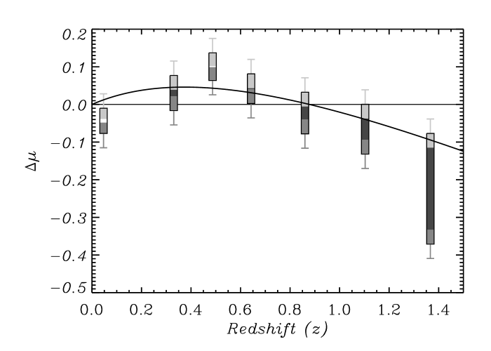
Figure 1.— The difference in the distance modulus, $\mu=5\log_{10}(d_{\lower 2.0pt\hbox{$\scriptstyle L$}})+25$, with $d_{\lower 2.0pt\hbox{$\scriptstyle L$}}$ in units Mpc, of the FB model with $H_{\lower 2.0pt\hbox{$\scriptstyle 0$}}=61.7\,\hbox{km}\;\,\hbox{sec}^{-1}\,\hbox{Mpc}^{-1}$, $\Omega_{\lower 2.0pt\hbox{$\scriptstyle M0$}}=0.326$ from that of an empty coasting Milne universe, with the same value of $H_{\lower 2.0pt\hbox{$\scriptstyle 0$}}$. The Riess et al. (2007) gold data set of 182 SneIa is binned using the criterion $n_{i}\Delta z_{i}=5.8$, where $n$ is the number of data points, and $\Delta z_{i}$ the width of the $i$th bin. The first bin boundary is set at $z=0.023$ as “Hubble bubble” points with $z\leq 0.023$ are excluded. Our bins are differ very slightly from those used in Fig. 6 of Riess et al. (2007): the single outlier point at $z=1.755$, falls in its own bin. This point which falls below the theoretical curve is not shown here, but is included in the $\chi^{2}$ analysis. We use the original distance moduli reported at http://braeburn.pha.jhu.edu/$\mathop{\sim}\limits$ariess/R06/sn_sample, without the suggested systematic subtraction of 0.32 mag, as we follow the Cepheid calibration of Sandage et al. (2006). The boxes show the standard statistical errors for the binned data using the reported uncertainties, which already account for luminosity corrections in the MLCS2k2 reduction (Jha et al., 2007). The whiskers indicate how the residuals move relative to the horizontal axis for the $2\sigma$ limits on $H_{\lower 2.0pt\hbox{$\scriptstyle 0$}}$ with $\Omega_{\lower 2.0pt\hbox{$\scriptstyle M0$}}=0.326$ fixed: light grey corresponds to the 2$\sigma$ upper bound, and dark grey to the 2$\sigma$ lower bound. The overlap in these two regions has been coloured black.

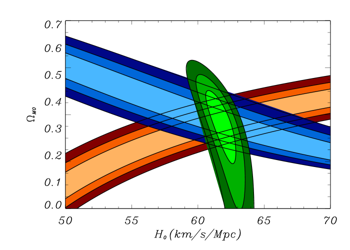
Figure 2.— 1$\sigma$, 2$\sigma$ and 3$\sigma$ confidence limits (oval contours) for fits of luminosity distances of type Ia supernovae (SneIa) in the Riess07 gold dataset (Riess et al., 2007) are compared to parameters within the ($\Omega_{\lower 2.0pt\hbox{$\scriptstyle M0$}}$,$H_{\lower 2.0pt\hbox{$\scriptstyle 0$}}$) plane which fit the angular scale of the sound horizon $\delta=0.01$ rad deduced for WMAP (Bennett et al., 2003; Spergel et al., 2007), to within 2%, 4% and 6% (contours running top–left to bottom–right); and to parameters which fit the effective comoving baryon acoustic oscillation (BAO) scale of $104h^{-1}$Mpc observed in galaxy clustering statistics (Cole et al., 2005; Eisenstein et al., 2005), to within 2%, 4% and 6% (contours running bottom–left to middle–right).

Ideally we should recompute the spectrum of Doppler peaks for the FB model. However, this requires considerable effort, as the standard numerical codes have been written solely for FLRW models, and every step has to be carefully reconsidered. This task is left for future work. The test that we apply here is to ask whether parameters exist for which the effective angular diameter scale of the sound horizon matches the angular scale of the sound horizon, $\delta=0.01$ rad, of the $\Lambda$CDM model, as determined by WMAP (Bennett et al., 2003). Since there is no change to the physics of recombination, but just an overall change to the calibration of cosmological parameters, this is entirely reasonable.

In Fig. 2 we plot parameter ranges which match the $\delta=0.01$ rad sound horizon scale to within 2%, 4% and 6%, using the calculation of the sound horizon given by Wiltshire (2007a, §7.2). The 2% contour would roughly correspond to the 2$\sigma$ limit if the WMAP uncertainties for the $\Lambda$CDM model are maintained. As this can only be confirmed by detailed computation of the Doppler peaks, the additional levels have been chosen cautiously. The limits shown have been arrived at assuming a volume–average baryon–to–photon ratio in the range $\eta_{\lower 2.0pt\hbox{$\scriptstyle B\gamma$}}=4.6$–$5.6\times 10^{-10}$ adopted by Tytler et al. (2000) prior to the release of WMAP1. With this range it is possible to achieve concordance with lithium abundances, while also better fitting helium abundances. This potentially resolves an anomaly. With the 2003 WMAP1 release (Bennett et al., 2003), the baryon–to–photon ratio was increased to the very upper range of values that had previously been considered, largely due to the consequence for the ratio of the heights of the first two Doppler peaks. This ratio of peak heights is sensitive to the mass ratio of baryons to non–baryonic dark matter – rather than directly to the baryon–to–photon ratio – as it depends physically on baryon drag in the primordial plasma. The fit to the Doppler peaks required more baryons than the range of Tytler et al. (2000) admitted, when calibrated with the FLRW model. In the FB calibration, on account of the difference between the bare and dressed density parameters, a bare value of ${\vphantom{\tilde{\Omega}}\bar{\Omega}}_{\lower 2.0pt\hbox{$\scriptstyle B0$}}\simeq 0.03$ nonetheless corresponds to a conventional dressed value $\Omega_{\lower 2.0pt\hbox{$\scriptstyle B0$}}\simeq 0.08$, and an overall mass ratio of baryonic matter to non–baryonic dark matter of about 1:3, which is larger than for $\Lambda$CDM. This would certainly indicate sufficient baryon drag to accommodate the ratio of the first two peak heights.

The final set of contours plotted in Fig. 2 relate to the independent test of the effective comoving scale of the baryon acoustic oscillation (BAO), as detected in galaxy clustering statistics (Cole et al., 2005; Eisenstein et al., 2005). Similarly to the case of the angular scale of the sound horizon, given that we do not have the resources to analyse the galaxy clustering data directly, we begin here with a simple but effective check. In particular, since the dressed geometry (3) does provide an effective almost–FLRW metric adapted to our clocks and rods in spatially flat regions, the effective comoving scale in this dressed geometry should match the corresponding observed BAO scale of $104h^{-1}$Mpc. We therefore plot parameter values which match this scale to within 2%, 4% or 6%.

The best–fit cosmological parameters, using SneIa only, are $H_{\lower 2.0pt\hbox{$\scriptstyle 0$}}=61.7^{+1.2}_{-1.1}\,\hbox{km}\;\,\hbox{sec}^{-1}\,\hbox{Mpc}^{-1}$ and ${f_{\hbox{\sevenrm v0}}}=0.76^{+0.12}_{-0.09}$, with 1$\sigma$ uncertainties. The values of the mean lapse function, bare density parameter, conventional dressed density parameter, mass ratio of non–baryonic dark matter to baryonic matter, bare Hubble parameter, effective dressed deceleration parameter and age of the universe measured in a galaxy are respectively: ${\vphantom{\tilde{\gamma}}\bar{\gamma}}_{\lower 2.0pt\hbox{$\scriptstyle 0$}}=1.381^{+0.061}_{-0.046}$; ${\vphantom{\tilde{\Omega}}\bar{\Omega}}_{\lower 2.0pt\hbox{$\scriptstyle M0$}}=0.125^{+0.060}_{-0.069}$; $\Omega_{\lower 2.0pt\hbox{$\scriptstyle M0$}}=0.33^{{}^{+}0.11}_{-0.16}$; $({\vphantom{\tilde{\Omega}}\bar{\Omega}}_{\lower 2.0pt\hbox{$\scriptstyle M0$}}-{\vphantom{\tilde{\Omega}}\bar{\Omega}}_{\lower 2.0pt\hbox{$\scriptstyle B0$}})/{\vphantom{\tilde{\Omega}}\bar{\Omega}}_{\lower 2.0pt\hbox{$\scriptstyle B0$}}=3.1^{+2.5}_{-2.4}$; ${\vphantom{\tilde{H}}\bar{H}}_{\lower 2.0pt\hbox{$\scriptstyle\!0$}}=48.2^{+2.0}_{-2.4}\,\hbox{km}\;\,\hbox{sec}^{-1}\,\hbox{Mpc}^{-1}$; $q=-0.0428^{+0.0120}_{-0.0002}$; $\tau_{\lower 2.0pt\hbox{$\scriptstyle 0$}}=14.7^{+0.7}_{-0.5}$ Gyr. Statistical uncertainties from the sound horizon and BAO tests cannot yet be given, but should significantly reduce the bounds on ${f_{\hbox{\sevenrm v0}}}$, $\Omega_{\lower 2.0pt\hbox{$\scriptstyle M0$}}$ etc.

One striking feature of Fig. 2 is that even if SneIa are disregarded, the parameters which fit the two independent tests relating to the sound horizon and the BAO scale agree with each other, to the accuracy shown, for values of the Hubble constant which include the value of Sandage et al. (2006). However, they do not agree for the values of $H_{\lower 2.0pt\hbox{$\scriptstyle 0$}}$ greater than $70\,\hbox{km}\;\,\hbox{sec}^{-1}\,\hbox{Mpc}^{-1}$ which best–fit the WMAP data (Bennett et al., 2003; Spergel et al., 2007) with the FLRW model.

The value of the Hubble constant quoted by Sandage et al. (2006) has been controversial, given the 14% difference from values which best–fit the WMAP data with the $\Lambda$CDM model (Bennett et al., 2003; Spergel et al., 2007). However, the WMAP analysis only constitutes a direct measurement of CMB temperature anisotropies; the determination of cosmological parameters involves model assumptions. We have removed the assumptions of the FLRW model, in an attempt to model the universe in terms of the distribution of galaxies that we actually observe, with an alternative proposal to averaging consistent with general relativity. Applied to the angular diameter of the sound horizon and the BAO scale this leads to different cosmological parameters: ones that agree with the measurement of Sandage et al. (2006).

The combination of best–fit cosmological parameters that arises is particularly interesting. The numerical value of present void volume fraction, ${f_{\hbox{\sevenrm v0}}}$, is identical to that of the dark–energy density fraction, $\Omega_{\lower 2.0pt\hbox{$\scriptstyle\Lambda 0$}}$, in the $\Lambda$CDM model with WMAP (Spergel et al., 2007). If the FB model is closer to the correct description of the actual universe, then in trying to fit a FLRW model, we appear to be led to parameters in which the cosmological constant is mimicking the effect of voids as far as the WMAP normalization to FLRW models is concerned. This it does imperfectly, since for a flat $\Lambda$CDM model $\Omega_{\lower 2.0pt\hbox{$\scriptstyle M0$}}=1-\Omega_{\lower 2.0pt\hbox{$\scriptstyle\Lambda 0$}}$, with the result that the best–fit value of $\Omega_{\lower 2.0pt\hbox{$\scriptstyle M0$}}$ normalized to the CMB does not match the best–fit value of $\Omega_{\lower 2.0pt\hbox{$\scriptstyle M0$}}$ for SneIa with the FLRW model, nor for other tests which directly probe $\Omega_{\lower 2.0pt\hbox{$\scriptstyle M0$}}$. For example, it has been recently noted that the values of the normalization of the primordial spectrum $\sigma_{\lower 2.0pt\hbox{$\scriptstyle 8$}}\mathop{\sim}\limits 0.76$ and matter content $\Omega_{\lower 2.0pt\hbox{$\scriptstyle M0$}}\mathop{\sim}\limits 0.24$ implied by WMAP3 are barely compatible with the abundances of massive clusters determined from X–ray measurements (Yepes et al., 2007). For the FB model, by contrast, the dressed density parameter, $\Omega_{\lower 2.0pt\hbox{$\scriptstyle M0$}}$, includes the range preferred in direct estimations of the conventional matter density parameter.

The integrated Sachs–Wolfe effect provides a further interesting test to be determined. Since the observed signal is based on a correlation to clumped structure (Boughn and Crittenden, 2004), for large scale averages any difference from the $\Lambda$CDM expectation would largely depend on the difference in expansion history of the two models. However, we might expect foreground voids to give anisotropies below the scale of homogeneity, for which evidence is seen (Rudnick et al., 2007).

In this Letter we have offered preliminary quantitative evidence, via agreement of independent cosmological tests, that the problem of “dark energy” might be resolved within general relativity. The differences in cosmological parameters inferred in the $\Lambda$CDM and FB models – including the average Hubble parameter and its variance, the expansion age, dressed matter density, baryon–to–photon ratio, baryon–to–dark matter ratio, CMB ellipticity – are such that the question as to which provides the better concordance model can be answered by future observations and new cosmological tests.

Acknowledgement This work was supported by the Marsden Fund of the Royal Society of New Zealand.

References

- Bennett et al. (2003) Bennett, C.L. et al. 2003, ApJ Suppl. 148, 1.
- Boughn and Crittenden (2004) Boughn, S. and Crittenden, R. 2004, Nature 427, 45.
- Buchert (2000) Buchert, T. 2000, Gen. Relativ. Grav. 32, 105.
- Buchert (2007) Buchert, T. 2007, arxiv:0707.2153.
- Cole et al. (2005) Cole, S. et al.2005, MNRAS 362 (2005) 505.
- Ellis (1984) Ellis, G.F.R. 1984, in General Relativity and Gravitation (eds B. Bertotti, F. de Felice and A. Pascolini), Dordrecht: Reidel, 215.
- Eisenstein et al. (2005) Eisenstein, D.J. et al. 2005, ApJ 633, 560.
- Gurzadyan et al. (2005) Gurzadyan, V.G. et al. 2005, Mod. Phys. Lett. A 20, 813.
- Gurzadyan et al. (2007) Gurzadyan, V.G. et al. 2007, Phys. Lett. A 363, 121.
- Hoyle and Vogeley (2004) Hoyle, F. and Vogeley, M.S. 2004, ApJ 607, 751.
- Jha et al. (2007) Jha, S., Riess, A.G. and Kirshner, R.P. 2007, ApJ 659, 122.
- Kass and Raftery (1995) Kass, R.E. and Raftery, A.E. 1995, J. Am. Statist. Assoc. 90, 773.
- Riess et al. (2007) Riess, A.G. et al. 2007, ApJ 659, 98.
- Rudnick et al. (2007) Rudnick, L., Brown S. and Williams, L.R. 2007, arXiv:0704.0908.
- Sandage et al. (2006) Sandage, A. et al. 2006, ApJ 653, 843.
- Spergel et al. (2007) Spergel, D.N. et al. 2007, ApJ Suppl. 170, 288.
- Tomita (2001) Tomita, K. 2001, MNRAS 326, 287.
- Trotta (2007) Trotta, R. 2007, MNRAS 378, 72.
- Tytler et al. (2000) Tytler, D., O’Meara, J.M., Suzuki, N. and Lubin, D. Phys. Scripta T85, 12 (2000).
- Wiltshire (2007a) Wiltshire, D.L. 2007a, New J. Phys. 9, 377.
- Wiltshire (2007b) Wiltshire, D.L. 2007b, Phys. Rev. Lett. in press; arxiv:0709.0732.
- Yepes et al. (2007) Yepes, G., Sevilla, R., Gottloeber S. and Silk, J. 2007, arxiv:0707.3230.