Tkachenko modes in a superfluid Fermi gas at unitarity

Abstract

We calculate the frequencies of the Tkachenko oscillations of a vortex lattice in a harmonically trapped superfluid Fermi gas. We use the elasto-hydrodynamic theory by properly accounting for the elastic constants, the Thomas-Fermi density profile of the atomic cloud, and the boundary conditions. Thanks to the Fermi pressure, which is responsible for larger cloud radii with respect to the case of dilute Bose-Einstein condensed gases, large vortex lattices are achievable in the unitary limit of infinite scattering length, even at relatively small angular velocities. This opens the possibility of experimentally observing vortex oscillations in the regime where the dispersion relation approaches the Tkachenko law for incompressible fluids and the mode frequency is almost comparable to the trapping frequencies.

Two component Fermi gases are very versatile systems, offering the possibility of exploring both fermionic and bosonic superfluidity. By exploiting Feshbach resonances to tune the interaction strength between different spin species, it is possible to realize ultracold gases of fermionic atoms and Bose-Einstein condensates (BECs) of dimers as well (for a recent review see Ref. giorgini07 ). Moreover, at resonance, where the interspecies scattering length diverges, fermionic atoms enter a new strongly correlated regime, the so-called unitary limit, in which the standard Bardeen-Cooper-Schrieffer (BCS) theory is not applicable. Here fermionic superfluidity is significantly enhanced, due to the stronger role played by the interactions. Vortex lattices have been already observed in this novel phase of matter zwierlein05 . The observation of vortices in Fermi gases represents a particularly important achievement, since the unambiguous detection of superfluidity in these systems is less straightforward than in the corresponding case of Bose-Einstein condensates.

In this paper we study the Tkachenko modes of the vortex lattice in a harmonically trapped Fermi gas at unitarity. These oscillations, originally studied in Ref. tkachenko66 for incompressible superfluids, correspond to shear distortions of the lattice planes and carry much lower energies than usual hydrodynamic modes. The investigation of Tkachenko modes in Bose-Einstein condensates has been largely pursued on both the theoretical anglin ; baym03 ; cozzini04 ; baksmaty04 ; mizushima04 ; sonin05 and experimental JILAtka ; JILALLL sides. An appealing reason to study vortex modes in Fermi gases at unitarity is given by the larger number of vortices $N_{v}$ achievable for a given rotation rate. As we shall discuss in the final part of this paper, unitary fermions of ⁶Li yield a significant enhancement (almost an order of magnitude) in the vortex number compared to bosonic atoms of ⁸⁷Rb. This is due to the large expansion of the cloud radius produced by the Fermi pressure. This effect provides the possibility of studying Tkachenko modes in a more systematic way than in the bosonic case, including an easier detection of modes with more than one radial node and the observation of Tkachenko modes at relatively small angular velocity $\Omega$, where the incompressible regime of the dispersion relation is exploited.

A first insight into the problem can be gained from the frequency spectrum of the Tkachenko oscillations of an infinite vortex lattice sonin87

$$\omega^{2}=\frac{c_{T}^{2}c_{s}^{2}k^{4}}{4\Omega^{2}+c_{s}^{2}k^{2}}\ ,$$ (1)

where $k$ is the wave vector, $c_{s}$ is the usual sound velocity, $c_{T}=\sqrt{\kappa\Omega/8\pi}$ is the Tkachenko velocity, and the limit $c_{s}\gg{}c_{T}$ is assumed. Here $\kappa=h/M$ is the quantum of circulation of a single vortex line, where $M=m$ for bosons and $M=2m$ for fermions, $m$ being the mass of the particles. The incompressible limit of Eq. (1) takes place for $c_{s}k\gg\Omega$ and corresponds to the original Tkachenko dispersion law $\omega=c_{T}k$. In the opposite limit $c_{s}k\ll\Omega$ one finds the quadratic dispersion relation $\omega=c_{T}c_{s}k^{2}/2\Omega$, characterizing the compressible limit of the spectrum. In a non-uniform configuration the actual values of $k$ are inversely proportional to the radius of the cloud and are fixed by the proper procedures of discretization that will be discussed later. In the experiments with BECs it is difficult to realize large vortex lattices at small angular velocities and the condition $c_{s}k\gg\Omega$ is hence hard to fulfill. Vice versa, we will show that in the case of fermions at unitarity the crossover from incompressible to compressible behavior can be more easily investigated.

In our calculation, we adapt the two-dimensional (2D) elasto-hydrodynamic treatment developed by Sonin sonin05 to the fermionic case. We consider two distinct density profiles in the Thomas-Fermi (TF) approximation: (i) the one corresponding to the cylinder geometry as considered in Ref. sonin05 and (ii) the 2D column density obtained by integrating a 3D TF cloud along the axial direction (hereafter also called pancake geometry). The cylinder geometry is an idealized configuration whose interest lies in the exact decoupling between the radial and axial dynamics. However, experimental situations are expected to be better described by the pancake geometry, which takes into account the 3D features of the inhomogeneous profile. While in the full 3D geometry the decoupling of dynamics is not exact, the axial motion is expected to be negligible for Tkachenko modes as long as vortices are straight. The use of the column density is hence expected to be a valuable approximation for pancake shape clouds which do not exhibit significant vortex bending.

One of the major differences between Bose and Fermi gases lies in the equation of state, being dominated in the Fermi case by the quantum pressure effect. In the TF approximation, the equation of state can be expressed as $\mu\propto{n}^{\gamma}$ in both cases, but with different values of the polytropic index $\gamma$. Here $\mu$ is the chemical potential and ${n}$ is the number density of particles. In 3D, $\gamma=1$ for bosons and $\gamma=2/3$ for fermions at unitarity note_pure2d , yielding a different TF density profile in the two cases. For a vortex lattice rotating at an angular velocity $\Omega$ in a harmonic trap with radial and axial frequencies $\omega_{\perp}$ and $\omega_{z}$, the coarse-grained equilibrium density profile is given by $n(\mbox{\boldmath$r$})\propto[\mu_{0}-\tilde{V}(\mbox{\boldmath$r$})]^{1/\gamma}$, where $\mu_{0}$ is the chemical potential for the trapped case, $\tilde{V}(\mbox{\boldmath$r$})\equiv m(\tilde{\omega}_{\perp}^{2}r_{\perp}^{2}+\omega_{z}^{2}z^{2})/2$ is the effective potential taking into account the centrifugal force, $\tilde{\omega}_{\perp}^{2}\equiv\omega_{\perp}^{2}-\Omega^{2}$, and $r_{\perp}^{2}\equiv{}x^{2}+y^{2}$.

For a TF configuration with pancake geometry we may reduce the problem to two dimensions by integrating out the $z$ coordinate; i.e., we employ the column density $n_{\rm 2D}(r_{\perp})=\int\mathrm{d}z\,{n}(\mbox{\boldmath$r$})$ as an effective 2D density profile. One hence finds $n_{\mathrm{2D}}(r_{\perp})\propto(\mu_{0}-m\tilde{\omega}_{\perp}^{2}r_{\perp}^{2}/2)^{1/\gamma_{\rm eff}}$ with $\gamma_{\rm eff}\equiv 2\gamma/(2+\gamma)$ corresponding to the equation of state $\mu\propto n^{\gamma_{\rm eff}}$ in the uniform 2D configuration. Note that the effective 2D polytropic index $\gamma_{\rm eff}$ always differs from the one calculated in the cylindrical geometry, where $\omega_{z}=0$ and $\gamma_{\rm eff}=\gamma$. It is also worth pointing out that $\gamma_{\rm eff}$ has the same value for fermionic systems in the cylindrical geometry and for bosonic systems in the pancake geometry (see Table 1). In the remainder of this paper, we treat the problem only in two dimensions and drop the subscript “$\perp$” of $r_{\perp}$ and the subscript “2D” of $n_{\rm 2D}$.

Macroscopic manifestations of superfluidity at zero temperature can be studied by resorting to the superfluid hydrodynamic equations. As long as we study the dynamics of vortices on length scales much larger than the intervortex distance, we can employ the elasto-hydrodynamic theory sonin76 ; baym83 ; sonin87 . Here the microscopic density and velocity fields are substituted by averaged quantities and the restoring force of the lattice is taken into account by adding an elastic energy term to the usual superfluid hydrodynamic energy functional note_bs .

The elastic energy for a triangular lattice is given by $E_{\textrm{el}}=\int\mathrm{d}{\mbox{\boldmath$r$}}\,\mathcal{E}_{\textrm{el}}$, where the energy density $\mathcal{E}_{\textrm{el}}$ in the rotating frame is $\mathcal{E}_{\mathrm{el}}=2C_{1}(\mbox{\boldmath$\nabla$}\cdot\mbox{\boldmath$\epsilon$})^{2}+C_{2}[\left(\partial\epsilon_{x}/\partial x-\partial\epsilon_{y}/\partial y\right)^{2}+\left(\partial\epsilon_{x}/\partial y+\partial\epsilon_{y}/\partial x\right)^{2}]$. Here $\epsilon$ is the vortex displacement field, and the coefficients $C_{1}$ and $C_{2}$ are the compressional and shear modulus respectively baym83 , corresponding to second derivatives of the energy density with respect to lattice distortions. They have to be calculated from the (microscopic) energy functional evaluated in the rotating frame baym83 .

In the Fermi case at unitarity the core size $\xi$ of vortices is of the order of the interparticle distance. Consequently, unless one works extremely close to the centrifugal limit antezza07 , $\xi$ is much smaller than the intervortex distance, which is of the order of the Wigner-Seitz radius of the vortex lattice cell, namely, $l_{\Omega}=\sqrt{\kappa/2\pi\Omega}=\sqrt{\hbar/M\Omega}$. This relation corresponds to the usual vortex density $n_{v}=1/\pi{}l_{\Omega}^{2}=2\Omega/\kappa$ obtained from the condition of quantized circulation. The elastic coefficients can then be calculated in the small core limit $\xi\ll{}l_{\Omega}$, equivalent to the Thomas-Fermi condition $\mu_{0}\gg\hbar\Omega$ comprcond . In this regime, the well-established result $C_{2}=-C_{1}={n}m\kappa\Omega/16\pi$ holds tkc2 ; baym83 ; sonin87 . Hence, for bosons $C_{2}=-C_{1}={n}\hbar\Omega/8$, while for fermions $C_{2}=-C_{1}={n}\hbar\Omega/16$, i.e., in the latter case ${n}$ is replaced by the density of pairs, ${n}/2$. This result can be understood by observing that fermionic pairs play the same role as bosonic molecules from the point of view of superfluidity.

Table 1: Effective polytropic index $\gamma_{\rm eff}$ in 2D for the bosonic and fermionic cases. For the cylindrical geometry, $\gamma_{\rm eff}=\gamma$, and for the pancake geometry, $\gamma_{\rm eff}=2\gamma/(2+\gamma)$. The values of the parameter $\alpha$ characterizing the dispersion law in the incompressible limit (see text) are also reported.

geometry	bosons	fermions
cylinder	1 ($\alpha=5.43$)	2/3 ($\alpha=5.59$)
pancake	2/3 ($\alpha=5.59$)	1/2 ($\alpha=5.75$)

We are finally ready to write the linearized elasto-hydrodynamic equations. In the rotating frame they take the form

$$\frac{\partial}{\partial t}\,\delta{n}+\mbox{\boldmath$\nabla$}\cdot({n}_{0}\,\delta\mbox{\boldmath$v$}) = 0\ ,$$ (2)

$$\frac{\partial}{\partial t}\,\delta\mbox{\boldmath$v$}+2\,\mbox{\boldmath$\Omega$}\wedge\delta\mbox{\boldmath$v$}+\mbox{\boldmath$\nabla$}\,\frac{\delta\mu}{m}-\frac{\mbox{\boldmath$F_{\textrm{el}}$}}{m{n}_{0}} = 0\ ,$$ (3)

$$\frac{\partial}{\partial t}\,\delta\mbox{\boldmath$v$}+2\,\mbox{\boldmath$\Omega$}\wedge\dot{\mbox{\boldmath$\epsilon$}}+\mbox{\boldmath$\nabla$}\,\frac{\delta\mu}{m} = 0\ ,$$ (4)

where $\dot{\mbox{\boldmath$\epsilon$}}=\partial\mbox{\boldmath$\epsilon$}/\partial t$ and the variation of the local chemical potential, $\delta\mu$, can be expressed in terms of the local sound velocity as $\delta\mu/m=(\partial\mu/\partial{n})\delta{n}/m=(c_{s}^{2}/{n}_{0})\delta{n}$. By combining Eqs. (3) and (4) one also finds $2m{n}_{0}\mbox{\boldmath$\Omega$}\wedge(\delta\mbox{\boldmath$v$}-\dot{\mbox{\boldmath$\epsilon$}})=\mbox{\boldmath$F_{\textrm{el}}$}$. Here ${n}_{0}\equiv{n}_{0}(\mbox{\boldmath$r$})$ is the equilibrium density, while $\delta{n}$ and $\delta\mbox{\boldmath$v$}$ are the density and velocity perturbations. The elastic force is given by ${(F_{\textrm{el}})}_{j}=\partial\sigma_{jk}/\partial{x_{k}}$, where $\sigma_{jk}=\delta{E}_{\textrm{el}}/\delta{u_{jk}}=\partial\mathcal{E}_{\textrm{el}}/\partial{u_{jk}}$ is the stress tensor defined in terms of the strain tensor $u_{jk}=(\partial\epsilon_{j}/\partial{x_{k}}+\partial\epsilon_{k}/\partial{x_{j}})/2$ baym83 . Note that, while in the case of BECs for the cylindrical geometry the ratio $c_{s}^{2}/{n}_{0}$ is constant and commutes with the gradient in Eqs. (3) and (4), this is not the case for $\gamma_{\rm eff}\neq 1$.

We are interested in the axisymmetric Tkachenko modes. In polar coordinates all the physical quantities are then independent of the azimuthal angle $\phi$ and we can reduce to ordinary differential equations with respect to $r$. For large vortex numbers one can approximate $\dot{\epsilon}_{\phi}\simeq\delta{v}_{\phi}$ (see Ref. sonin05 ) and the above linearized equations take the simplified form

$$2i\omega\Omega\,\delta{v}_{r} = -\omega^{2}\delta{v}_{\phi}-\frac{c_{T}^{2}}{{n}_{0}}\frac{1}{r^{2}}\frac{\partial}{\partial r}\left[{n}_{0}r^{3}\frac{\partial}{\partial r}\left(\frac{\delta{v}_{\phi}}{r}\right)\right]\ ,\quad$$ (5)

$$2i\omega\Omega\,\delta{v}_{\phi} = \frac{\partial}{\partial r}\left[\frac{c_{s}^{2}}{{n}_{0}}\frac{1}{r}\frac{\partial}{\partial r}\left({n}_{0}r\delta{v}_{r}\right)\right]\ ,$$ (6)

where $\delta{v}_{r}$ and $\delta{v}_{\phi}$ are the radial and azimuthal components of $\delta\mbox{\boldmath$v$}$, and $c_{T}=\sqrt{\kappa\Omega/8\pi}=l_{\Omega}\Omega/2$.

We solve Eqs. (5) and (6) with proper boundary conditions at the cloud center and at the cloud radius $R=\sqrt{2\mu/m\tilde{\omega}_{\perp}^{2}}$ using the shooting method. At $r=0$ the velocity must vanish: $\delta{v}_{r}(0)=\delta{v}_{\phi}(0)=0$. Following the same arguments of Ref. sonin05 , we obtain at $r=R$

$$\frac{\partial}{\partial{r}}\delta{v}_{\phi}(R)-\frac{\delta{v}_{\phi}(R)}{R} = 0\ ,$$ (7)

$$\frac{\partial}{\partial{r}}\delta{v}_{r}(R)+\frac{\delta{v}_{r}(R)}{R} = -\frac{\gamma_{\rm eff}}{\gamma_{\rm eff}+1}\frac{i\omega\Omega R}{c_{s}^{2}(0)}\delta{v}_{\phi}(R)\ .$$ (8)

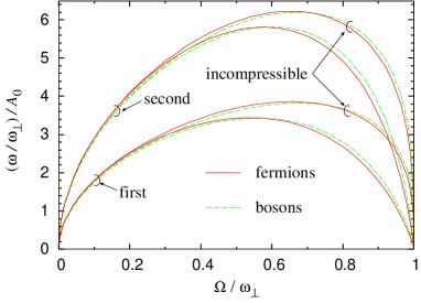
Figure 1: (Color online) Plot of the frequency $\omega$ of the first and the second axisymmetric Tkachenko modes as a function of the angular velocity. The green dashed line corresponds to pancake bosons ($\gamma_{\mathrm{eff}}=2/3$), while the red solid line to pancake fermions ($\gamma_{\mathrm{eff}}=1/2$). For each mode the incompressible limit $\omega_{\mathrm{inc}}=\omega_{0}\alpha$ is shown for comparison.

In Fig. 1 we present our predictions for the frequencies of the two lowest Tkachenko modes at unitarity. In the numerical calculation it is natural to solve Eqs. (5) and (6) for the dimensionless ratio $\omega/\omega_{0}$, where $\omega_{0}=c_{T}/R$. Since the discretized values of $k$ are proportional to $1/R$ the frequency $\omega_{0}$ is basically the analogue of the incompressible limit $c_{T}k$ of Eq. (1). Comparison with the homogeneous spectrum of Eq. (1) then shows that $\omega/\omega_{0}$ is the analogue of $c_{s}k/\sqrt{4\Omega^{2}+c_{s}^{2}k^{2}}$, i.e., of the factor responsible for compressibility effects. The dependence of $\omega_{0}$ on the angular velocity can be expressed analytically. The radius of the cloud is given by $R=R_{0}/(1-\tilde{\Omega}^{2})^{\nu}$, where $R_{0}$ is the radius of the non-rotating cloud, $\tilde{\Omega}=\Omega/\omega_{\perp}$, and $\nu=[2(\gamma_{\mathrm{eff}}+1)]^{-1}$. Then, $\omega_{0}=A_{0}\omega_{\perp}\sqrt{\tilde{\Omega}}(1-\tilde{\Omega}^{2})^{\nu}$, where $A_{0}=\sqrt{m/4M}a_{\perp}/R_{0}$ and $a_{\perp}=\sqrt{\hbar/m\omega_{\perp}}$. The full dependence of $\omega$ on $\Omega$ is hence displayed by plotting the quantity $\omega/A_{0}\omega_{\perp}$ which does not depend any longer on $R_{0}$, but only on the ratio $\Omega/\omega_{\perp}$. In the figure we also report the predictions for a dilute Bose-Einstein condensed gas in the same pancake configuration. The differences are actually very small, showing that, when expressed in the units of Fig. 1, the results for the Tkachenko frequencies do not depend in an appreciable way on the actual form of the equation of state which instead can significantly affect the value of the TF radius and hence of $A_{0}$.

One can get a qualitative understanding of the dependence of $\omega$ on $\Omega$ in the trapped case looking at the homogeneous dispersion relation (1). To this purpose, one has to evaluate $c_{s}$ and $k$ in the finite size system. A simple estimate for the sound velocity is given by its value at the center of the cloud, i.e., $c_{s}^{2}\sim\gamma_{\mathrm{eff}}\mu/m=\gamma_{\mathrm{eff}}\tilde{\omega}_{\perp}^{2}{R}^{2}/2$. The effective wave vector can instead be quantized proportionally to $1/{R}$, where the proportionality coefficient can be extracted by comparing Eq. (1) with the numerical calculation. For a general value of $\Omega$, the latter result would depend on the chosen estimate for $c_{s}$. However, in the $\Omega\to 0$ limit Eq. (1) becomes independent of $c_{s}$ and one can unambiguously define $k=\alpha/R$ with $\alpha=\lim_{\Omega\to 0}\omega/\omega_{0}$. The quantized value of $k$ can then be used to estimate the full $\Omega$ dependence using Eq.(1). This procedure was first exploited by Baym baym03 in the case of BECs and yields a rather accurate estimate of the whole dispersion law sound . We find that the value of $\alpha$ exhibits only a weak dependence on $\gamma$ and on the geometry employed (see Table 1). For the lowest Tkachenko mode we find the value $\alpha=5.75$ for fermions in the pancake geometry to be compared with the result $\alpha=5.59$ holding for bosons in the same geometry (or for fermions in the cylindrical geometry) alpha . Note also that the incompressible limit $\omega_{\mathrm{inc}}=\omega_{0}\alpha$ of the dispersion relation reproduces the full dispersion with high accuracy up to values $\tilde{\Omega}=0.4\sim 0.5$ of the angular velocity (see Fig. 1).

Let us now discuss the dependence of the number of vortices $N_{v}$ on the experimental parameters. This is important in order to determine the physical regimes of $\Omega/\omega_{\perp}$ achievable in practice. The number of vortices in the TF approximation is $N_{v}=n_{v}\pi{}{R}^{2}$. For a harmonically trapped Fermi gas at unitarity one has 2D=3D $R=a_{\perp}[2\sqrt{1+\beta}(3N\lambda)^{1/3}]^{1/2}(1-\tilde{\Omega}^{2})^{-1/3}$, where $\beta\simeq-0.6$ is a universal dimensionless parameter accounting for the role of interactions qmc , $N$ is the number of particles, and $\lambda=\omega_{z}/\omega_{\perp}$ is the trap aspect ratio. Thus, $N_{v}(\mbox{fermions})=4\sqrt{1+\beta}\,\tilde{\Omega}(1-\tilde{\Omega}^{2})^{-2/3}(3N\lambda)^{1/3}$. Using the corresponding expression for a Bose-Einstein condensed gas we find

$$\frac{N_{v}(\mbox{fermions})}{N_{v}(\mbox{bosons})}=\frac{4\sqrt{1+\beta}}{(1-\tilde{\Omega}^{2})^{1/15}}\frac{(3N\lambda)_{f}^{1/3}}{(15N\lambda{}a/a_{\perp})_{b}^{2/5}}\ ,$$ (9)

where the subscripts refer to bosons and fermions and $a$ is the $s$-wave scattering length. For $(N\lambda)_{f}=(N\lambda)_{b}$ the above ratio becomes $4\sqrt{1+\beta}\ [3N\lambda(1-\tilde{\Omega}^{2})]^{-1/15}(5a/a_{\perp})_{b}^{-2/5}$ and the small exponent $-1/15$ implies that the result is practically insensitive to the value of $\tilde{\Omega}$, $N$, and $\lambda$. On the other hand, in typical BECs one has $a/a_{\perp}\ll 1$, so that $N_{v}(\mbox{fermions})/N_{v}(\mbox{bosons})$ can be significantly larger than 1 radius .

In the JILA experiments on BECs one has $\lambda=0.63$, $a\simeq 5\,$nm, $a_{\perp}=3.74\,\mu$m, and $N\sim 10^{6}$ JILAtka . This yields $N_{v}(^{87}\mathrm{Rb})=43.7\tilde{\Omega}(1-\tilde{\Omega}^{2})^{-3/5}$. In the MIT experiments, at unitarity one has $\lambda=0.40$ and $N\sim 10^{6}$ zwierlein05 . Then $N_{v}(^{6}\mathrm{Li})/N_{v}(^{87}\mathrm{Rb})\simeq 6.1(1-\tilde{\Omega}^{2})^{-1/15}$, which corresponds to the significant gain in the number of vortices mentioned in the introduction note_3body .

The increase of $N_{v}$ at unitarity allows to measure Tkachenko modes at relatively small angular velocities. For example, a fermionic cloud with the above parameters easily contains more than $100$ vortices at $\tilde{\Omega}=0.4$, deeply in the incompressible region of the spectrum. The maximum of the frequency of the lowest Tkachenko mode takes place at $\tilde{\Omega}\simeq 0.55$ and corresponds to $\omega/\omega_{\perp}\simeq 0.13$ for the same parameters. This value is quite larger than the highest frequency observed in ⁸⁷Rb experiments, namely, $\omega/\omega_{\perp}=0.023$ at $\tilde{\Omega}=0.84$ JILAtka . This provides promising perspectives for precision measurements of Tkachenko modes note_imaging , for a direct determination of the quantum of circulation in Fermi superfluids, and for the general investigation of the incompressible regime of the dispersion relation, whose quantitative analysis in experiments is a long standing question in the field of superfluid systems.

- (1) S. Giorgini, L. P. Pitaevskii, and S. Stringari, arXiv:0706.3360 [cond-mat.soft].
- (2) M. W. Zwierlein, J. R. Abo-Shaeer, A. Schirotzek, C. H. Schunk, and W. Ketterle, Nature (London)435, 1047 (2005).
- (3) V. K. Tkachenko, Zh. Eksp. Teor. Fiz. 50, 1573 (1966) [Sov. Phys. JETP 23, 1049 (1966)].
- (4) J. R. Anglin and M. Crescimanno, cond-mat/0210063.
- (5) G. Baym, Phys. Rev. Lett. 91, 110402 (2003).
- (6) M. Cozzini, L. P. Pitaevskii, and S. Stringari, Phys. Rev. Lett. 92, 220401 (2004).
- (7) E. B. Sonin, Phys. Rev. A71, 011603(R) (2005).
- (8) L. O. Baksmaty, S. J. Woo, S. Choi, and N. P. Bigelow, Phys. Rev. Lett. 92, 160405 (2004).
- (9) T. Mizushima, Y. Kawaguchi, K. Machida, T. Ohmi, T. Isoshima, and M. M. Salomaa, Phys. Rev. Lett. 92, 060407 (2004).
- (10) I. Coddington, P. Engels, V. Schweikhard, and E. A. Cornell, Phys. Rev. Lett. 91, 100402 (2003).
- (11) V. Schweikhard, I. Coddington, P. Engels, V. P. Mogendorff, and E. A. Cornell, Phys. Rev. Lett. 92, 040404 (2004).
- (12) E. B. Sonin, Rev. Mod. Phys. 59, 87 (1987).
- (13) In the pure 2D situation, where ( is the axial trap frequency) and the 2D equation of state holds, for both Bose and Fermi gases.
- (14) E. B. Sonin, Zh. Eksp. Teor. Fiz. 70, 1970 (1976) [Sov. Phys. JETP 43, 1027 (1976)].
- (15) G. Baym and E. Chandler, J. Low Temp. Phys. 50, 57 (1983).
- (16) In the case of Fermi superfluids, there exist fermionic bound states localized in the vortex cores caroli64 whose energy, at unitarity, is of order of the Fermi energy sensarma06 . Since the Tkachenko modes have much smaller energy, the coupling between these two kinds of excitations can be safely ignored.
- (17) C. Caroli, P. G. De Gennes, and J. Matricon, Phys. Lett. 9, 307 (1964).
- (18) R. Sensarma, M. Randeria, T.-L. Ho, Phys. Rev. Lett. 96, 090403 (2006).
- (19) M. Antezza, M. Cozzini, and S. Stringari, Phys. Rev. A75, 053609 (2007).
- (20) This condition should not be confused with the condition characterizing the incompressible limit of the Tkachenko dispersion law.
- (21) V. K. Tkachenko, Zh. Eksp. Teor. Fiz. 56, 1763 (1969) [Sov. Phys. JETP 29, 945 (1969)].
- (22) The estimate becomes even more accurate if one employs the sound velocity averaged over the whole cloud baym03 .
- (23) For one recovers the value corresponding to the incompressible 2D result of Ref. anglin (see note_pure2d ), also confirmed in Refs. cozzini04 ; sonin05 . We also note that the value for the bosonic column density, corresponding to a 3D pancake geometry, agrees with the value extracted from the 3D sum rule calculation of Ref. cozzini04 .
- (24) The radius of the 2D column density clearly coincides with the radial radius of the 3D TF profile.
- (25) J. Carlson, S.-Y. Chang, V. R. Pandharipande, and K. E. Schmidt, Phys. Rev. Lett. 91, 050401 (2003); G. E. Astrakharchik, J. Boronat, J. Casulleras, and S. Giorgini, ibid. 93, 200404 (2004).
- (26) Since the Tkachenko frequency scales like , the larger value of quenches the Tkachenko frequency at fixed . For example, for the experimental values considered in the text, the value of for bosons is about a factor larger than for fermions. However, as we shall see later, this quenching can be largely compensated by choosing relatively small rotation rates.
- (27) In principle, one can increase in BECs by employing larger values of and/or . However, three-body recombination losses become crucial for large and/or , which makes difficult to obtain very large vortex lattices unless one works close to the centrifugal limit.
- (28) Due to the extremely small vortex core size, the imaging of vortices in atomic Fermi gases at unitarity is actually a non-trivial issue. This difficulty can be overcome by ramping the scattering length to small and positive values just before the expansion.