Fractional Hamiltonian Monodromy from a Gauss-Manin Monodromy

Abstract.

Fractional Hamiltonian Monodromy is a generalization of the notion of Hamiltonian Monodromy, recently introduced by N. N. Nekhoroshev, D. A. Sadovskií and B. I. Zhilinskií for energy-momentum maps whose image has a particular type of non-isolated singularities. In this paper, we analyze the notion of Fractional Hamiltonian Monodromy in terms of the Gauss-Manin Monodromy of a Riemann surface constructed from the energy-momentum map and associated to a loop in complex space which bypasses the line of singularities. We also prove some propositions on Fractional Hamiltonian Monodromy for $1:-n$ and $m:-n$ resonant systems.

1. Introduction

We consider an integrable system on a four dimensional symplectic manifold defined by an energy-momentum map. For a proper map, the Liouville-Arnold theorem allows to foliate the phase space by tori or a disjoint union of tori over the regular values of the image of the map. Hamiltonian monodromy is the monodromy of this fibration [Dui80, CB97]. The word Hamiltonian is added to distinguish this monodromy from the Gauss-Manin monodromy of Riemann surfaces which is also used in this paper. A non trivial monodromy can be expected if the set of regular values of the image of the energy-momentum map is not simply connected. Hamiltonian monodromy has profound implications both in classical and quantum mechanics [Ngoc99] since it is the simplest topological obstruction to the existence of global action-angle variables [Dui80] and thus of global good quantum numbers [Ngoc99]. The phenomenon of Hamiltonian monodromy has been exhibited in a large variety of physical systems both in classical and quantum mechanics [AKE04, SC00, KR03, CWT99, SZ99, WJD03, GCSZ04, EJS04].

The presence of non-trivial monodromy in energy-momentum maps with isolated singularities of focus-focus type is now well-established. The non-trivial monodromy in the spherical pendulum is due to this singularity [Dui80, CB97]. Recently, the definition of Hamiltonian monodromy has been extended to characterize not only isolated singularities but also some types of non-isolated singularities, leading to the concept of Fractional Hamiltonian Monodromy [NSZ02, NSZ06, Efs04, ECS07]. More precisely, one considers an energy-momentum map with a 1-dimensional set $C$ of weak critical values defined by the property that each point of this set lifts to a particular type of singular torus, a curled torus, i.e. for the simplest case two cylinders glued together along a line whose extremities are identified after a half-twist. The standard Hamiltonian monodromy describes the possible non-triviality of a 2-torus bundle over a loop in the set of regular values of the image of the energy-momentum map. The monodromy matrix is an automorphism of the first homology group $H_{1}$ of the torus with integer coefficients. Fractional monodromy can appear if the set of admissible paths is enlarged to include loops which cross the singular line $C$. For such paths, the singularity of $C$ being sufficiently weak, it can be shown that the monodromy action can still be defined but only on a subgroup of $H_{1}$. The formal extension of this action to the whole group leads to monodromy matrices with fractional coefficients and to the denomination fractional monodromy. One of the main motivations for the introduction of this new concept is given by the quantum manifestation of monodromy in the discrete joint spectrum of the energy-momentum map [Ngoc99, NSZ06]. This spectrum can be represented as a lattice of points in $\mathbb{R}^{2}$. The focus-focus singularity can be detected by a point defect of this lattice which prevents it to be a regular lattice isomorphic to $\mathbb{Z}^{2}$. In the same way, fractional monodromy can be interpreted as a line defect of the lattice and appears therefore as a natural generalization of standard hamiltonian monodromy.

The presence of fractional monodromy has been shown in a system of coupled oscillators in $m:-n$ resonance with $m$ or $n$ different from 1. Two constructions have been given based on geometric [NSZ06, Nek07] or analytic [ECS07] arguments to define rigorously the crossing of $C$. The geometric construction consists in following a basis of cycles of a regular torus through the crossing of $C$. Not all the cycles can cross continuously the singularity, only those corresponding to a subgroup of $H_{1}$ can. When $C$ is crossed, one allows cycles to break up and reconnect, the orientation of the cycles being preserved. The second construction uses, as in the original paper of Duistermaat [Dui80, CB97], the period lattice of the torus [Arn89] which is however not defined on the singular line $C$. The period lattice is defined through two functions $\Theta$ and $T$ at each point of the regular values of the image of the energy-momentum map. Some regularizations of these functions can be made in order to cross continuously the line of singularities [ECS07]. Note that the preceding geometric point of view can be reconstructed from this analytic approach since the basis of cycles can be determined from the functions $\Theta$ and $T$.

The goal of this work is to study fractional monodromy by complexifying the phase space in order to bypass the line of singularities. Somewhat similar studies for the Lagrange top and the spherical pendulum have already been published [Aud02, Viv03, BC01] and have highlighted the relation between Hamiltonian and complex monodromy. A parallel can also be made with Bohr-Sommerfeld rules for semi-classical quantization. Such calculations can be undertaken in the $C^{\infty}$ [dVP99, Ngoc00, dVN03] or in the analytic context [Vor83, DDP97, DP97]. The real approach needs regularization of the sub-principal term whereas the complex approach avoids such problems by avoiding the singularity. In this paper, we show that fractional hamiltonian monodromy is given by a Gauss-Manin monodromy [AGZV88, Zol06] of a Riemann surface constructed from the energy-momentum map. The construction can be made in the reduced phase space [CB97] which is well suited to the introduction of Riemann surfaces. The Gauss-Manin connection is defined for a complex semi-circle around the line $C$ of singularities and can be calculated by applying the Picard-Lefschetz theory. We also introduce the complex extension of the functions $\Theta$ and $T$ which are viewed as integrals of rational forms over a cycle of the Riemann surface. In other words, the regularizations of $\Theta$ and $T$ in the real approach are replaced by a complex continuation of these functions. The variations of $\Theta$ and $T$ along the bypass in the complex domain are deduced from the Gauss-Manin monodromy. The functions $\Theta$ and $T$ allow us to go back to the real approach and to define a real monodromy. We show that this monodromy corresponds to fractional hamiltonian monodromy asymptotically in the limit where the radius of the complex semi-circle goes to 0. Using this construction, we recover the results of the real approach obtained in Refs. [NSZ02, NSZ06, Efs04, ECS07] for the 1:-2 resonance and Ref. [Nek07] for $m:-n$ resonance. Moreover, for $1:-n$ and $m:-n$ resonant systems, we give new proofs of these results from the real and the complex approaches. A geometric point of view of the Gauss-Manin monodromy can be given by inspecting the motion of the branching points of the Riemann surface along the semi-circle around $C$. For $1:-n$ resonant systems, the Riemann surface has locally $n$ complex branching points in a neighborhood of $C$ lying on a circle around the origin with an angle of $2\pi/n$ between each other. Along a complex semi-circle around $C$, the $n$ points turn by an angle of $2\pi/n$ and exchange their positions. The variation of $\Theta$ near $C$ is then calculated as a residue of a given 1-form. This characterizes the line of singularities $C$ and fractional monodromy.

The organization of this article is as follows : We first consider the real approach and we determine the monodromy matrices for 1:-2, $1:-n$ and $m:-n$ resonances in Sec. 2. We next show in Sec. 3 how fractional monodromy can be defined in the complex approach and we detail its geometric interpretation. We recover the different results obtained in the real approach. Concluding remarks and perspectives are given in Sec. 4. Appendices A and B present a schematic representation of the geometric construction of fractional monodromy for 1:-2 and $1:-n$ resonant systems in the real approach and the semi-classical point of view for $1:-n$ and $m:-n$ resonances. The material of these appendices complements the existing literature on these two points. Appendix C finally deals with the reduction procedure in the complex approach.

2. The real approach

The goal of this section is to furnish a short overview of fractional hamiltonian monodromy in the real approach. Starting from the example introduced in Ref. [Efs04, ECS07] for the 1:-2 resonance, we extend it to $1:-n$ and $m:-n$ resonances. The core of the results presented in this section are already contained in [NSZ02, NSZ06, Efs04, ECS07]. We describe it in some detail since we need the results for the complex approach. Furthermore, we present analytic computations in this section and a geometric construction in appendix A which are slightly different from the original ones and give a new view on fractional hamiltonian monodromy. The originality of the analytical computation for the 1:-2 resonance relies in the introduction of a local description of the energy-momentum map near the origin of the bifurcation diagram which considerably simplifies the computation of the monodromy matrix. Since these arguments are generalizable to $1:-n$ and $m:-n$ resonances, they allow us to prove some propositions stated in [NSZ06, Efs04, Nek07]. For the geometric description, we introduce the standard representation of a torus i.e. a rectangle whose some edges are identified. This geometric construction can be extended straightforwardly to $1:-n$ resonant systems.

2.1. The 1:-2 resonance

We consider the symplectic manifold $M=T^{*}\mathbb{R}^{2}$ with standard symplectic form $\omega=dq_{1}\wedge dp_{1}+dq_{2}\wedge dp_{2}$. We introduce the energy-momentum map $F=(H,J):M\to\mathbb{R}^{2}$ where the two functions $J$ and $H$ have zero Poisson brackets $\{J,H\}=0$. Following Refs. [NSZ02, NSZ06, Efs04, ECS07], we choose a system corresponding to the $1:-2$ resonance defined by

(3) $$\left\{\begin{array}[]{ll}H=\sqrt{2}[\left(q_{1}^{2}-p_{1}^{2}\right)p_{2}+2q_{1}p_{1}q_{2}]+2\varepsilon(q_{1}^{2}+p_{1}^{2})(q_{2}^{2}+p_{2}^{2})\\ J=\frac{1}{2}\left(q_{1}^{2}+p_{1}^{2}\right)-\left(q_{2}^{2}+p_{2}^{2}\right)\end{array}\right.\ ,$$

where $\varepsilon$ is a non-zero real number. We denote by $\mathcal{R}$ the image of $F$ and by $\mathcal{R}_{reg}$ the regular values of $\mathcal{R}$. We recall that a point $M\in\mathcal{R}$ is regular if the 1-forms $dH$ and $dJ$ are linearly independent at all points of $F^{-1}(h,j)$.

The flow of $J$ defines an $S^{1}$-action on the phase space but this action is not principal since the isotropy groups of the points $\{p_{1}=0,q_{1}=0,p_{2},q_{2}\}$ are isomorphic to $\mathbb{Z}/2\mathbb{Z}$. The reduced phase space $J^{-1}(j)/S^{1}$ can be constructed by using the algebra of invariant polynomials with values in $\mathbb{R}$ which is generated by [Efs04, CB97] :

(8) $$\left\{\begin{array}[]{llll}J({\bf p,q})=1/2\left(q_{1}^{2}+p_{1}^{2}\right)-\left(q_{2}^{2}+p_{2}^{2}\right)\\ \pi_{1}({\bf p,q})=1/2\left(q_{1}^{2}+p_{1}^{2}\right)+\left(q_{2}^{2}+p_{2}^{2}\right)\\ \pi_{2}({\bf p,q})=\sqrt{2}[\left(q_{1}^{2}-p_{1}^{2}\right)q_{2}-2q_{1}p_{1}p_{2}]\\ \pi_{3}({\bf p,q})=\sqrt{2}[\left(q_{1}^{2}-p_{1}^{2}\right)p_{2}+2q_{1}p_{1}q_{2}]\end{array}\right.\ ,$$

with the constraint $|J|\leq\pi_{1}$. The reduced phase spaces $P_{j}=J^{-1}(j)/S^{1}$ are defined in the space $\mathbb{R}^{3}=\left(\pi_{1},\pi_{2},\pi_{3}\right)$ by the equations :

(9) $$\pi_{2}^{2}+\pi_{3}^{2}=\left(\pi_{1}-j\right)\left(\pi_{1}+j\right)^{2}\ ,$$

and correspond to non-compact surfaces with a conical singularity for $j<0$. Having introduced the invariant polynomials, some comments can be made on the choice of $H$. Since $\{H,J\}=0$, it can be shown that if $H$ is polynomial in $\left(p_{i},q_{i}\right)$ then it can be written as a polynomial function in $J$, $\pi_{1}$, $\pi_{2}$ and $\pi_{3}$. We also notice that the reduced phase space for the 1:-2 resonance being non-compact, not every choice of $H$ leads to a proper map for the energy-momentum map $F=(H,J)$. This explains why a term of degree four has been added to $H$ [see Eq. (3)]. The image of the energy-momentum map defined by Eq. (3) has the particularity to present a line of singularities $C$, each point of this line except the origin lifts to a singular curled torus (the origin lifts to a pinched-curled torus). The topology of these singular tori can be determined by the intersection of the reduced phase space $P_{j}$ with the level set $H_{j}=h$ (see Sec. 2.4). $H_{j}$ is the reduced Hamiltonian, i.e., a map from $P_{j}$ to $\mathbb{R}$ that sends a point of $P_{j}$ to $H(\pi_{1},\pi_{2},\pi_{3},j)$. Moreover, since the two energy-momentum maps $F=(H,J)$ and $F^{\prime}=(H-f(J),J)$, where $f$ is a polynomial function, define up to a diffeomorphism the same fibration of the phase space, we can consider an example such that $H=0$ for the line of singularities $C$. Figure 1 displays the bifurcation diagram of $F$ (see [Efs04, ECS07] for details on this construction).

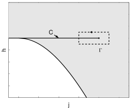
Figure 1. Image $\mathcal{R}$ of the energy-momentum map $F$ (in grey). The singular line $C$ is represented by the horizontal solid line. The small full dot indicates the position of the image of the pinched-curled torus. A loop $\Gamma$ crossing transversally $C$ is depicted in dashed lines.

Singular points (i.e. not regular) are represented by solid lines in Fig. 1. $C$ is a line of weak singularities. The word weak means that for each point of $C$, there exist points of the corresponding pre-image such that the rank of $F$ is 1. We recall that for a regular point, the rank of $F$ is always equal to 2 and that the rank of $F$ is 0 for one point of $F^{-1}(0,0)$.

2.2. Fractional Hamiltonian Monodromy

We begin this section by recalling some basic facts about integer and fractional monodromy. The word hamiltonian in hamiltonian monodromy will be omitted when confusion is unlikely to occur.

Standard or integer monodromy is defined for a loop $\Gamma$ along regular values of $\mathcal{R}$. Fractional monodromy is obtained by extending the possible loops, allowing them to cross some particular type of weak singular lines such as $C$. In the standard case, we consider a point $(h,j)$ of $\Gamma$ which lifts to a torus $T^{2}(h,j)$. We fix a basis of the homology group $H_{1}(T^{2}(h,j),\mathbb{Z})$. There exists a natural connection of the torus bundle which allows to transport this basis along $\Gamma$ [CB97, Bat91]. The monodromy matrix, which is an automorphism of $H_{1}$, is the holonomy of this connection. This construction can be generalized to fractional monodromy but only a subgroup of $H_{1}(T^{2}(h,j),\mathbb{Z})$ can be transported continuously across the line $C$ [NSZ06, ECS07]. These remarks can be understood by the following construction. Let $(h,j)\in\mathcal{R}_{reg}$. Denoting by $\varphi_{J}$ and $\varphi_{H}$ the flows associated to the Hamiltonians $J$ and $H$, the period lattice of $F$ at a point $(h,j)$ is the set

(10) $$\{(t_{1},t_{2})\in\mathbb{R}^{2}|\varphi_{J}^{t_{1}}\circ\varphi_{H}^{t_{2}}(z)=z\}\ ,$$

for all $z\in F^{-1}(h,j)$. A basis for this period lattice, which is isomorphic to $\mathbb{Z}^{2}$, is given by the vectors $v_{1}=(2\pi,0)$ and $v_{2}=(-\Theta,T)$ where $\Theta$ is the rotation angle and $T$ the first return time of the flow $\varphi_{H}$ defined as follows [Dui80, CB97]. The Hamiltonian $J$ generates an $S^{1}$-action on $F^{-1}(h,j)$. We denote by $\theta$ an angle conjugated to the action $J$. Following $\varphi_{J}$ which is parameterized by $\theta$, one goes back to the starting point when $\theta$ increases by $2\pi$, which gives $v_{1}$. If we consider now $\varphi_{H}$ from a point of an orbit of the flow $\varphi_{J}$, one sees that the first intersection of these two flows takes places at time $T$. The two points of intersection of the two flows define two angles $\theta_{f}$ and $\theta_{i}$ and the twist $\Theta=\theta_{f}-\theta_{i}$ which is determined with respect to the direction of $\varphi_{J}$. Note that a different choice of the angle $\theta$ leads to a different basis for the period lattice. The corresponding rotation angles $\Theta$ differ by a multiple of $2\pi$. The monodromy matrix associated to a loop lying in the regular values of the image of the energy-momentum map is related to the behavior of the functions $\Theta$ and $T$ along this loop. For the standard monodromy, after a counterclockwise loop around an isolated critical value (focus-focus singularity) it can be shown that the rotation angle is increased by $2\pi$ whereas the first return time is unchanged. As a consequence, $v_{1}$ is transformed into $v_{1}$ and $v_{2}$ into $-v_{1}+v_{2}$, and thus the monodromy matrix $M$ written in the local basis $(v_{1},v_{2})$ is equal to

(13) $$M=\left(\begin{array}[]{cc}1&0\\ -1&1\end{array}\right)\ .$$

The two functions $\Theta$ and $T$ allow to define a basis of cycles for the homology group $H_{1}(F^{-1}(h,j),\mathbb{Z})$ and thus to recover a more geometric point of view. A basis $([\beta_{1}],[\beta_{2}])$ of $H_{1}(F^{-1}(h,j),\mathbb{Z})$ is given by the cycles associated respectively to the flows of the vector fields

(16) $$\left\{\begin{array}[]{ll}X_{1}=2\pi X_{J}\\ X_{2}=-\Theta(h,j)X_{J}+T(h,j)X_{H}\end{array}\right.\ .$$

The flows $\varphi_{X_{1}}^{t}$ ($t\in[0,1]$) and $\varphi_{X_{2}}^{t}$ ($t\in[0,1]$) generate respectively the closed cycles $\beta_{1}$ and $\beta_{2}$. These two cycles are schematically represented in Fig. 2 for $\Theta=-\pi$. In the basis $([\beta_{1}],[\beta_{2}])$, the monodromy matrix is given by the same matrix as Eq. (13) obtained for the period lattice.

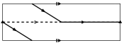
Figure 2. Schematic representation on the torus $F^{-1}(h,j)$ of the cycles $\beta_{1}$ and $\beta_{2}$ depicted respectively in dashed and solid lines.

The situation is slightly more complicated for fractional monodromy. The analytic construction of fractional monodromy follows the same steps as for the standard case [ECS07]. Returning to the example of Eq. (3) and considering the loop $\Gamma$ of Fig. 1, the question which naturally arises is the definition of the crossing of the line $C$ since $\Theta$ has a discontinuity of size $\pi$ on this line and $T$ diverges. The idea of the method proposed in Ref. [ECS07] consists in prolonging by continuity the function $\Theta$ (the continuous function is called $\tilde{\Theta}$) and in rescaling the time to obtain a finite first return time denoted $\tau$. Note that this rescaling does not modify the definition of the cycles but only the time to cover them. This leaves therefore the monodromy matrix unchanged. $\tilde{\Theta}$ is defined by $\tilde{\Theta}(h,j)=\Theta(h,j)$ for points $(h,j)$ of $\Gamma$ before the crossing of the line $C$ and by $\tilde{\Theta}(h,j)=\Theta(h,j)+\pi$ for points after [ECS07]. A basis of the period lattice is given by the vectors $v_{1}=(2\pi,0)$ and $v_{2}=(-\tilde{\Theta},\tau)$ and the cycles $\beta_{1}$ and $\beta_{2}$ are now associated to the vector fields

(19) $$\left\{\begin{array}[]{ll}X_{1}=2\pi X_{J}\\ \tilde{X}_{2}=-\tilde{\Theta}(h,j)X_{J}+\tau(h,j)X_{H}\end{array}\right.\ .$$

The construction of these cycles has however to be carefully examined. $\varphi_{X_{1}}^{t}$ ($t\in[0,1]$) generates a cycle $\beta_{1}$ for all points of $\Gamma$. Before the crossing, $\varphi_{\tilde{X}_{2}}^{t}$ ($t\in[0,1]$) generates a closed cycle $\beta_{2}$ but after the crossing, $\varphi_{\tilde{X}_{2}}^{t}$ ($t\in[0,1]$) generates only half of a cycle. To get a complete cycle, we thus have to take $t\in[0,2]$. This means geometrically that only a cycle $\beta_{2}$ covered twice can be transported continuously across the line $C$. Thus, not all cycles in the homology group can be transported along $\Gamma$. Only a subgroup corresponding to the cycles that are run twice by $\tilde{X}_{2}$ can be transported. In terms of the period lattice, the crossing of $C$ is only possible for the sublattice generated by $v_{1}$ and $2v_{2}$. We can then define the monodromy matrix for a counterclockwise loop crossing transversally $C$ once. The monodromy matrix $M$ reads in the basis $(v_{1},2v_{2})$ or in the basis $([\beta_{1}],[2\beta_{2}])$

(22) $$M=\left(\begin{array}[]{cc}1&0\\ -1&1\end{array}\right)\ .$$

Extending formally the definition of $M$ to the whole homology group or the whole period lattice, we obtain in the basis $(v_{1},v_{2})$ or in the basis $([\beta_{1}],[\beta_{2}])$

(25) $$M=\left(\begin{array}[]{cc}1&0\\ -\frac{1}{2}&1\end{array}\right)\ .$$

We finally note that this generalized monodromy is still topological in the sense that it depends only on the homotopy equivalence class of the loop considered. We also point out that these cycles prolonged continuously to the curled torus allow to recover the geometric construction of fractional monodromy described in appendix A.

2.3. Local computation of the monodromy matrix

The determination of the monodromy matrix is based on the behavior of the functions $\Theta$ and $\tau$ on the line of singularities $C$. More precisely, the monodromy matrix can be constructed uniquely from the size of the discontinuity of $\Theta$ and from the fact that $\tau$ is continuous. In Ref. [ECS07], the computation was done by using global expressions for $\Theta$ and $\tau$ in terms of elliptic integrals. It is clear that such a global calculation can be expected to be done explicitly only for simple energy-momentum maps.

We propose a computation of the fractional monodromy matrix based on local arguments for the energy-momentum map $F$, i.e., a Puiseux expansion in $h$ and $j$ around $(h=0,j=0)$. This expansion is not trivial because a particular dissymmetry in $h$ and $j$ has to be preserved.

Lemma 1.

In the variables $(\pi_{1},\pi_{2},\pi_{3},J)$ and for a point $(h,j)\in\mathcal{R}_{reg}$, the functions $\Theta$ and $\tau$ are given by the following expressions :

(26) $$\Theta(h,j)=h\int_{\pi_{1}^{-}}^{\pi_{1}^{+}}\frac{d\pi_{1}}{(j+\pi_{1})\sqrt{Q(\pi_{1})}}\ ,$$

and

(27) $$\tau(h,j)=\frac{1}{2}\int_{\pi_{1}^{-}}^{\pi_{1}^{+}}\frac{j+\pi_{1}}{\sqrt{Q(\pi_{1})}}d\pi_{1}\ ,$$

where $Q(\pi_{1})$ is a polynomial given by

(28) $$Q(\pi_{1})=(\pi_{1}-j)(\pi_{1}+j)^{2}-[h-\varepsilon(\pi_{1}^{2}-j^{2})]^{2}\ .$$

$\pi_{1}^{+}$ and $\pi_{1}^{-}$ are the two largest real roots of $Q$ with $\pi_{1}^{-}<\pi_{1}^{+}$.

Proof see [ECS07] and Sec. (2.5) for a more general construction. We recall that $\tau$ is the first return time of the flow of the rescaled vector field $\frac{1}{q_{1}^{2}+p_{1}^{2}}X_{H}$.$\Box$

Proposition 1.

The monodromy matrix for a counterclockwise oriented loop $\Gamma$ crossing once the line $C$ transversally at a point different from the origin (see Fig. 1) is given by

(31) $$M=\left(\begin{array}[]{cc}1&0\\ -1/2&1\end{array}\right)\ .$$

Proof The monodromy matrix is given by the behavior of $\Theta$ and $\tau$ in the neighborhood of the line $C$. Taking $j<0$ fixed and finite, the limits $\lim_{h\to 0^{\pm}}\Theta(h,j)$ and $\lim_{h\to 0^{\pm}}\tau(h,j)$ have been calculated in [ECS07]. Elliptic integrals and asymptotic expansions of these integrals were used.

We propose a simpler computation by considering the asymptotic limit $j\to 0$. For that purpose, we analyze the roots of the polynomial $Q$ as $h$ and $j$ go to zero. Since a qualitative change of the functions $\Theta$ and $\tau$ is expected when the polynomial $Q$ has a multiple complex root, we determine the complex discriminant locus of $Q$ near the origin $h=j=0$. This point will be made clearer with the introduction of Riemann surfaces in Sec. 3 but here it gives the way in which the two limits $h\to 0$ and $j\to 0$ should be taken. The discriminant locus in the real approach has already been calculated since it corresponds to the line of singularities of the bifurcation diagram, i.e., to the points where the 1-forms $dH$ and $dJ$ are linearly dependent (see Fig. 1). We introduce the variable $x=j+\pi_{1}$ and $h$, $j$ and $x$ are taken complex. Three roots of $Q$ vanish for $h=j=0$.

Let us assume that $x$, $j$ and $h$ go to zero. Constructing the Newton polyhedron associated to $Q$ [Kir93], we obtain the principal part $Q_{N}$ of $Q$ which can be written as

(32) $$Q_{N}=x^{3}-2jx^{2}-h^{2}\ .$$

We notice that this principal part is symmetric with respect to $h$ which is not the case for the polynomial $Q$. Simple algebra leads to the following asymptotic discriminant locus

(35) $$\left\{\begin{array}[]{ll}h=\pm\sqrt{j^{3}(-\frac{32}{27})}\\ h=0\end{array}\right.\ ,$$

denoted $\Delta$. This complex locus is displayed for $j\in\mathbb{R}$ in Fig. 8. Equation (32) also shows that the weights 2, 2 and 3 can respectively be attributed to $x$, $j$ and $h$. In other words, if we introduce the small parameter $r$, the principal parts of $x$, $j$ and $h$ can be written

(39) $$\left\{\begin{array}[]{lll}x_{N}=\bar{x}r^{2}\\ j_{N}=\bar{j}r^{2}\\ h_{N}=\bar{h}r^{3}\end{array}\right.\ .$$

The monodromy can be computed along a small loop in $\mathcal{R}$ around the origin. This loop can be parameterized by $(\bar{h},\bar{j})\in S^{1}$ which allows to derive a local version of the computation of fractional monodromy. We thus let $\bar{h}\to 0$ while keeping $\bar{j}$ fixed and finite. Note that it is equivalent to consider the limits $h,j\to 0$ with the condition $h=o(j^{3/2})$, since on $\Delta$ we have asymptotically $h=O(j^{3/2})$. In order to determine the leading terms of the roots of $Q$ in this case, we construct the Newton polygon of $Q_{N}$. The approximate solutions fulfill

(40) $$-2\bar{j}\bar{x}^{2}-\bar{h}^{2}=0\ .$$

Since the sum of the three roots of $Q$ that go to zero when $h,j\to 0$ is $2j$, and the sum of the four roots is $\frac{1}{\varepsilon^{2}}$, one deduces that the principal parts of the roots are given in the original variables by

(45) $$\left\{\begin{array}[]{llll}x_{1}=2j\\ x_{2}=\frac{-h}{\sqrt{-2j}}\\ x_{3}=\frac{h}{\sqrt{-2j}}\\ x_{4}=\frac{1}{\varepsilon^{2}}\end{array}\right.\ .$$

These expressions can be compared with the ones given in Ref. [ECS07] where $j<0$ is fixed and $h\to 0$ :

(50) $$\left\{\begin{array}[]{llll}x_{1}=2j\\ x_{2}=\frac{-h}{\sqrt{-2j}+2\varepsilon j}\\ x_{3}=\frac{h}{\sqrt{-2j}-2\varepsilon j}\\ x_{4}=2j+\frac{1}{\varepsilon^{2}}+\frac{2\varepsilon h}{1+2\varepsilon^{2}j}\end{array}\right.\ .$$

We now calculate $\lim_{\bar{h}\to 0^{\pm},\bar{j}<0}\Theta(h,j)$ and $\lim_{\bar{h}\to 0,\bar{j}<0}\tau(h,j)$. We consider first $h>0$ and $j<0$. $\Theta(h,j)$ can be written as

(51) $$\Theta(h,j)=\frac{h}{i\varepsilon}\int_{x_{3}}^{x_{4}}\frac{dx}{x\sqrt{(x-x_{1})(x-x_{2})(x-x_{3})(x-x_{4})}}\ .$$

We determine only the principal term of the asymptotic expansion of $\Theta$. The symbol $\sim$ represents the equivalence in the limit $h\to 0$, $j\to 0$ and $h=o(j^{3/2})$. From Eqs. (45), we obtain

(52) $$\Theta(h,j)\sim\frac{h}{i\varepsilon}\int_{h/\sqrt{-2j}}^{1/\varepsilon^{2}}\frac{dx}{x\sqrt{(x-2j)(x+h/\sqrt{-2j})(x-h/\sqrt{-2j})(x-1/\varepsilon^{2})}}\ .$$

We decompose the preceding integral into three integrals by introducing the terms $k$ and $k^{\prime}$ which go to 0 such that $\frac{|h|}{\sqrt{-2j}}\ll k\ll-2j\ll k^{\prime}\ll 1$. $k$ and $k^{\prime}$ are chosen for instance as $j^{\alpha}$. The notation $a\ll b$ means that the ratio $a/b\to 0$ as $a$ and $b$ go to 0. The three integrals are taken over the intervals $[|h|/\sqrt{-2j},k]$, $[k,k^{\prime}]$ and $[k^{\prime},1/\varepsilon^{2}]$. It can be shown that the limit of the last two integrals is zero. The first integral reads

(53) $$\Theta(h,j)\sim\frac{h}{i\varepsilon}\int_{h/\sqrt{-2j}}^{k}\frac{dx}{x\sqrt{(-2j)(x^{2}-h^{2}/(-2j))(-1/\varepsilon^{2})}}\ ,$$

which can be rewritten as

(54) $$\Theta(h,j)\sim h\int_{h/\sqrt{-2j}}^{k}\frac{dx}{x\sqrt{(-2j)(x^{2}-h^{2}/(-2j))}}\ .$$

The change of variables $x=\frac{h}{\sqrt{-2j}}u$ leads to

(55) $$\Theta(h,j)\sim\int_{1}^{+\infty}\frac{du}{u\sqrt{u^{2}-1}}\ .$$

Using the fact that

(56) $$\int\frac{du}{u\sqrt{u^{2}-1}}=\arctan[\sqrt{u^{2}-1}]\ ,$$

one finally arrives to

(57) $$\lim_{h\to 0^{+},j\to 0^{-},h=o(j^{3/2})}\Theta(h,j)=\frac{\pi}{2}\ .$$

Similar calculations for $h<0$ give

(58) $$\lim_{h\to 0^{-},j\to 0^{-},h=o(j^{3/2})}\Theta(h,j)=\frac{-\pi}{2}\ .$$

We then deduce that the discontinuity of $\Theta$ is equal to $\pi$.

$\tau$ can be calculated along the same lines. This time the first two terms go to zero and we only determine the last one

(59) $$\tau(h,j)\sim\frac{1}{2i\varepsilon}\int_{k^{\prime}}^{1/\varepsilon^{2}}\frac{xdx}{\sqrt{(x-x_{1})(x-x_{2})(x-x_{3})(x-x_{4})}}\ .$$

Simple algebra leads to

(60) $$\tau(h,j)\sim\frac{1}{2i\varepsilon}\int_{k^{\prime}}^{1/\varepsilon^{2}}\frac{dx}{\sqrt{x(x-1/\varepsilon^{2})}}\ ,$$

and using the fact that

(61) $$\int\frac{dx}{\sqrt{x(x-1/\varepsilon^{2})}}=2\ln[\sqrt{x}+\sqrt{x-1/\varepsilon^{2}}]\ ,$$

one obtains that

(62) $$\lim_{h\to 0^{\pm},j\to 0^{-},h=o(j^{3/2})}\tau(h,j)=\frac{-\pi}{2\varepsilon}\ .$$

$\tau$ is therefore continuous on the line $C$. The monodromy matrix is finally deduced from the behavior of $\Theta$ and $\tau$ in the neighborhood of $C$. We follow for that purpose the construction of Ref. [ECS07] which is briefly recalled in Sec. 2.2.$\Box$

Remark 1.

The preceding computation being local does not show the topological character of fractional monodromy i.e. its independence with respect to the homotopically equivalent loops considered or more simply with respect to $j$. This point has been proved in the real approach in Ref. [ECS07] and will be proved in the complex approach in Sec. 3.

2.4. $1:-n$ resonant system

We consider the energy-momentum map $F=(H,J)$ where $J$ is given by

(63) $$J=\frac{1}{2}[(p_{1}^{2}+q_{1}^{2})-n(q_{2}^{2}+p_{2}^{2})]\ ,$$

with $n\geq 2$. We assume that the bifurcation diagram of $F$ is locally in the neighborhood of the origin given by Fig. 3. The singular locus corresponds to ($h=0,j\leq 0$). Each point of this locus lifts to a singular torus i.e. a pinched-curled torus for the origin and an $n-$curled torus for the other points. A $k$-curled torus is a singular torus for which one cycle is covered k-times while the others only once.

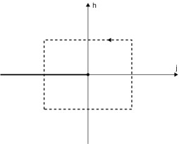
Figure 3. Local bifurcation diagram in the neighborhood of the origin $(h=0,j=0)$ for the $1:-n$ resonant system. The singular locus is represented by the large solid line. The small full dot indicates the position of the origin. The dashed line depicts a loop used to calculate the fractional monodromy matrix.

We now restrict the discussion to a particular family of energy-momentum maps having locally the bifurcation diagram of Fig. 3. As in Sec. 2.2, the first step consists in determining the invariant polynomials associated to the momentum $J$. We have [Efs04]

(68) $$\left\{\begin{array}[]{llll}J({\bf p,q})=1/2[m\left(q_{1}^{2}+p_{1}^{2}\right)-n\left(q_{2}^{2}+p_{2}^{2}\right)]\\ \pi_{1}({\bf p,q})=1/2[m\left(q_{1}^{2}+p_{1}^{2}\right)+n\left(q_{2}^{2}+p_{2}^{2}\right)]\\ \pi_{2}({\bf p,q})=\sqrt{n^{m}m^{n}}\Re[(q_{1}+ip_{1})^{n}(q_{2}+ip_{2})^{m}]\\ \pi_{3}({\bf p,q})=\sqrt{n^{m}m^{n}}\Im[(q_{1}+ip_{1})^{n}(q_{2}+ip_{2})^{m}]\end{array}\right.\ ,$$

for $m\geq 1$ and $n\geq 1$. The reduced phase space $P_{j}$ is defined by

(69) $$\pi_{2}^{2}+\pi_{3}^{2}=(\pi_{1}+j)^{n}(\pi_{1}-j)^{m}\ ,$$

with the condition $\pi_{1}\geq|j|$.

Definition 1.

We consider the set $\mathcal{F}$ of energy-momentum maps $F=(J,H)$ which can be written as

(72) $$F=\left\{\begin{array}[]{ll}J\\ H=\pi_{3}+R(\pi_{1},J)\\ \end{array}\right.\ ,$$

where $R$ is a polynomial so that $F$ is a proper map. $\pi_{1}$, $\pi_{3}$ and $J$ are given by Eqs. (68) for $m=1$.

Note that we do not search to determine or characterize the set $\mathcal{F}$. Only some properties of the elements of $\mathcal{F}$ will be sufficient to compute the monodromy matrix. Simple examples can be exhibited to show that $\mathcal{F}$ is not empty. For instance for the resonance 1:-3, we can choose

(75) $$F=\left\{\begin{array}[]{ll}J\\ H=\pi_{3}-(\pi_{1}-J)(\pi_{1}+J)^{4}\\ \end{array}\right.\ .$$

We are interested in the local behavior of $R$ near the origin or in other words under which conditions on $R$, the image of the corresponding energy-momentum map is given by Fig. 3.

Lemma 2.

The energy-momentum map given by Eqs. (72) has locally the bifurcation diagram of Fig. 3 in a neighborhood of the origin if the polynomial $R$ is of the form

(76) $$R(\pi_{1},J)=(\pi_{1}+J)^{n^{\prime}}(\pi_{1}-J)^{m^{\prime}}\tilde{R}(\pi_{1},J)\ ,$$

where $n^{\prime}$ and $m^{\prime}$ are positive integers such that $n^{\prime}>\frac{n}{2}$ and $n^{\prime}+m^{\prime}>\frac{n+1}{2}$. $\tilde{R}$ is a polynomial in $\pi_{1}$ and $J$ such that the two smallest real positive roots of the polynomial $Q$ which are larger than $j$ for $(h,j)\in\mathcal{R}_{reg}$ are simple roots . $Q$ is the polynomial defined by

(77) $$Q=(\pi_{1}+j)^{n}(\pi_{1}-j)-[h-R(\pi_{1},j)]^{2}\ .$$

The two roots are denoted $\pi_{1}^{-}$ and $\pi_{1}^{+}$ with $\pi_{1}^{-}<\pi_{1}^{+}$.

Proof The proof is based on the nature of the intersection of the reduced phase space $P_{j}$ with the level sets $\{H_{j}=h\}$ of equations $h=\pi_{3}+R(\pi_{1},j)$ as $h$ and $j$ vary. Fig. 4 displays these intersections for three different values of $h$, $j<0$ being fixed. The case considered in this figure is the 1:-3 resonance and the energy-momentum map of Eqs. (75). Fig. 4 represents the generic topology of the level sets $\{H_{j}=h\}$ which we are going to characterize. We recall that each point of the reduced phase space lifts in the original phase space to a circle except for the point of coordinates $(\pi_{1}=-j,\pi_{2}=0,\pi_{3}=0)$ which lifts either to a circle covered $n$ times, if $j<0$, or to a point, if $j=0$. One deduces from the bifurcation diagram of $F$ that the intersection of the level set $\{H_{j}=h\}$ with $P_{j}$ contains a circle passing through the singular point $S=(\pi_{1}=-j,\pi_{2}=0,\pi_{3}=0)$, for $j\leq 0$ and $h=0$. We set $y=\pi_{3}$, $x=\pi_{1}+j$ and $x^{\prime}=\pi_{1}-j$. The local behavior near the point $S$ of the two surfaces is given by

(78) $$y=\pm x^{\frac{n}{2}}x^{\prime\frac{1}{2}}\ ,$$

for $P_{j}$ and by

(79) $$y=-R(\pi_{1},j)\ ,$$

for $\{H_{j}=0\}$. It is then straightforward to show that the local behavior expected is obtained if $R(\pi_{1},j)=x^{n^{\prime}}x^{\prime m^{\prime}}\tilde{R}(\pi_{1},j)$ with the conditions $n^{\prime}>\frac{n}{2}$ and $n^{\prime}+m^{\prime}>\frac{n+1}{2}$, $m^{\prime}\geq 0$. The first and second inequalities result respectively from the conditions for $j<0$ and $j=0$.$\Box$

Remark 2.

The inequalities of lemma 2 are strict to ensure that a multiplication by a constant factor of the term $R$ does not modify the local behavior of the image of the energy-momentum map. This point has not been assumed for the 1:-2 resonance, the parameter $\varepsilon$ is thus chosen sufficiently small in this case. Here, this hypothesis simplifies the computation of the monodromy matrix as can be seen in the proofs of lemma 4 and proposition 2.

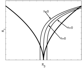
Figure 4. Intersections of the reduced phase space $P_{j}$ (in large solid lines) with the level sets $H_{j}=h$ for $h>0$, $h=0$ and $h<0$ in the plane $\pi_{2}=0$. The energy-momentum map corresponding to this diagram is given by Eqs. (75).

Proposition 2.

The monodromy matrix of a 1:-n resonant system of the form (72) is given for a loop turning counterclockwise around the origin (see Fig. 3) and crossing once transversally the line $C$ by

(82) $$M=\left(\begin{array}[]{cc}1&0\\ -1/n&1\end{array}\right)\ .$$

Remark 3.

Propositions 2 and 3 (see Sec. 2.5) were formulated as conjectures in Refs. [NSZ06, Efs04]. They are based on the analysis of the quantum joint spectrum of the energy-momentum maps. They have been recently proved in Ref. [Nek07] from a geometrical construction. Note also that our starting point here and in Sec. 2.5 is more general than in Sec. 2.2 in the sense that only a local structure of the bifurcation diagram of the energy-momentum map $F=(H,J)$ is assumed.

As was done for the 1:-2 resonance, we have to determine the expressions of the functions $\Theta$ and $\tau$ in terms of the invariant polynomials, the monodromy matrix being given by the behavior of these two functions in the neighborhood of $C$.

Lemma 3.

The functions $\Theta$ and $\tau$ are given for a point $(h,j)\in\mathcal{R}_{reg}$ by the following integrals

(85) $$\left\{\begin{array}[]{ll}\Theta(h,j)=\int_{\pi_{1}^{-}}^{\pi_{1}^{+}}\frac{h}{j+\pi_{1}}\frac{d\pi_{1}}{\sqrt{Q}}+\Theta_{0}(h,j)\\ \tau(h,j)=\frac{1}{n}\int_{\pi_{1}^{-}}^{\pi_{1}^{+}}\frac{(j+\pi_{1})^{n-1}}{\sqrt{Q}}d\pi_{1}\\ \end{array}\right.\ .$$

$\Theta_{0}$ is a function over $\mathcal{R}$ which is continuous on the line of singularities $C$ and which therefore gives a trivial contribution to the monodromy matrix. $\tau$ is the first return time of the rescaled vector field $X=\frac{1}{(p_{1}^{2}+q_{1}^{2})^{n-1}}{X_{H}}$.

Proof By definition, we have for a point $(h,j)\in\mathcal{R}_{reg}$ that [ECS07]

(86) $$\Theta(h,j)=\int_{0}^{T}\dot{\theta}dt\ ,$$

where $\theta$ is the angle variable conjugate to $J$. It can be expressed in terms of the variables $(q_{1},p_{1})$ by

(87) $$\theta=\arg(p_{1}+iq_{1})\ .$$

This corresponds to a particular choice of the angle $\theta$. Other choices lead to the same monodromy matrix. This point will be detailed in Sec. 2.5 for the $m:-n$ resonance. Differentiating Eq. (87) and using Hamilton’s equations, one arrives to

(88) $$\dot{\theta}=\frac{n\pi_{3}+\frac{\partial R}{\partial p_{1}}p_{1}+\frac{\partial R}{\partial q_{1}}q_{1}}{q_{1}^{2}+p_{1}^{2}}\ ,$$

which simplifies into

(89) $$\dot{\theta}=\frac{1}{j+\pi_{1}}(nh-nR+\frac{\partial R}{\partial p_{1}}p_{1}+\frac{\partial R}{\partial q_{1}}q_{1})\ .$$

The integral of Eq. (86) can be rewritten as an integral in the reduced phase space $P_{j}$ [ECS07] :

(90) $$\Theta(h,j)=2\int_{\pi_{1}^{-}}^{\pi_{1}^{+}}\dot{\theta}\frac{d\pi_{1}}{\dot{\pi_{1}}}\ .$$

Using the particular form of the polynomial $R$ (see lemma 2), it can be shown that the last three terms of Eq. (89) give a continuous contribution to the function $\Theta$ denoted $\Theta_{0}$. Since $\dot{\pi}_{1}=2n\pi_{2}$ [Efs04], we finally obtain that

(91) $$\Theta(h,j)=\int_{\pi_{1}^{-}}^{\pi_{1}^{+}}\frac{h}{j+\pi_{1}}\frac{d\pi_{1}}{\sqrt{Q}}+\Theta_{0}(h,j)\ .$$

The term $\pi_{2}$ has been replaced in Eq. (91) by combining Eqs. (69) and (75).

The determination of $\tau$ is straightforward if we remark that

(92) $$\tau(h,j)=\int_{0}^{\tau}ds=\int_{0}^{T}\frac{ds}{dt}dt=\int_{0}^{T}(p_{1}^{2}+q_{1}^{2})^{n-1}dt\ ,$$

where $s$ and $t$ are respectively the rescaled and the original time. The rest of the proof consists, as we did for $\Theta$, in rewriting the integral of Eq. (92) in the reduced phase space $P_{j}$ and leads to

(93) $$\tau(h,j)=\frac{1}{n}\int_{\pi_{1}^{-}}^{\pi_{1}^{+}}\frac{(j+\pi_{1})^{n-1}}{\sqrt{Q}}d\pi_{1}\ .$$

$\Box$ The last technical point to be discussed is the behavior of the roots of $Q$ as $h$ go to zero.

Lemma 4.

The complex discriminant locus $\Delta$ of $Q$ near the origin $(h=0,j=0)$ is given by

(96) $$\Delta=\left\{\begin{array}[]{ll}h=0\\ h=\pm\sqrt{-n^{n}j^{n+1}\frac{2^{n+1}}{(n+1)^{(n+1)}}}\\ \end{array}\right.\ .$$

The polynomial $Q$ as a function of $x$ and in the limit $h\to 0$, $j<0$ fixed has $n$ roots $x_{k}$ whose leading term reads

(97) $$x_{k}=\frac{h^{2/n}}{(-2j)^{1/n}}e^{2i\pi k/n}\ ,$$

with $k\in\{0,1,2,...,n-1\}$. The other roots of $Q$ have a non-zero finite limit.

Proof We first determine the complex discriminant locus $\Delta$ of $Q$ near the point $(h=0,j=0)$. Constructing the Newton polyhedron of $Q$ and taking into account only the terms of lower degrees, the principal part $Q_{N}$ of $Q$ can be written

(98) $$Q_{N}(x)=x^{n+1}-2jx^{n}-h^{2}\ .$$

A straightforward calculation then leads to $\Delta$.

In the limit $h\to 0$, $j<0$ fixed, we construct the Newton polygon associated to $Q$. The roots of the principal part of $Q_{N}$ satisfy $-2jx^{n}=h^{2}$ which allows to deduce the $n$ roots $x_{k}$ ($k\in\{0,1,\cdots,n-1\}$).$\Box$

We have now all the tools ready to prove proposition 2.

Proof We first consider the case $h>0$ and $j<0$. We recall some of the properties of the roots of the polynomial $Q$ viewed as a function of $x$ which will be used in the calculation. We assume that $Q$ has $N$ roots with $N>n$, denoted $x_{i}$ ($i\in\{0,1,\cdots N-1\}$). $x_{n},x_{n+1},\cdots,x_{N-1}$ are the roots of $Q$ of order 1 in the limit $h\to 0$, $j<0$ fixed. $x_{n}$ is the smallest real positive root of $Q$ with a non-zero limit. Since the polynomial $R$ is defined up to a multiplicative constant, we can write $Q$ without loss of generality as follows $Q(x)=\prod_{i=0}^{i=N-1}(x-x_{i})$. Examination of the coefficients of $Q$ leads to the following relations

(102) $$\left\{\begin{array}[]{lll}\prod_{i=0}^{i=N-1}x_{i}=(-1)^{N+1}h^{2}\\ \prod_{i=0}^{n-1}x_{i}=(-1)^{n-1}\frac{h^{2}}{(-2j)}\\ \prod_{i=n}^{N-1}x_{i}=2j(-1)^{N-n+1}\\ \end{array}\right.\ .$$

We determine only an equivalent of the function $\Theta-\Theta_{0}$. We obtain

(103) $$\Theta(h,j)-\Theta_{0}(h,j)\sim h\int_{\frac{|h|^{2/n}}{(-2j)^{1/n}}}^{x_{n}}\frac{dx}{x\sqrt{\prod_{i=0}^{i=N-1}(x-x_{i})}}\ ,$$

where $\frac{|h|^{2/n}}{(-2j)^{1/n}}$ is the smallest positive real root of $Q$. We introduce the function $k$ such that $\frac{|h|^{2/n}}{(-2j)^{1/n}}\ll k\ll 1$ when $h\to 0$. We then proceed as in the proof for the resonance 1:-2 by decomposing the integral of Eq. (103) into two integrals. Only the first integral from $\frac{|h|^{2/n}}{(-2j)^{1/n}}$ to $k$ has a limit different from zero. We then have

(104) $$\Theta(h,j)-\Theta_{0}(h,j)\sim h\int_{\frac{|h|^{2/n}}{(-2j)^{1/n}}}^{k}\frac{dx}{x\sqrt{(-2j)(x^{n}-\frac{h^{2}}{-2j})\times 1}}\ .$$

The change of variables $x=\frac{|h|^{2/n}}{(-2j)^{1/n}}u$ leads to the following expression for $\Theta-\Theta_{0}$

(105) $$\Theta(h,j)-\Theta_{0}(h,j)\sim\int_{1}^{+\infty}\frac{du}{u\sqrt{u^{n}-1}}\ .$$

Using the fact that

(106) $$\int\frac{du}{u\sqrt{u^{n}-1}}=\frac{2}{n}\arctan[\sqrt{u^{n}-1}]\ ,$$

one finally arrives to

(107) $$\lim_{h\to 0^{+},j<0}\Theta(h,j)-\Theta_{0}(h,j)=\frac{\pi}{n}\ .$$

It can also be shown that

(108) $$\lim_{h\to 0^{-},j<0}\Theta(h,j)-\Theta_{0}(h,j)=\frac{-\pi}{n}\ .$$

Following the same arguments, we can calculate the limit of $\tau$. We decompose $\tau$ into two integrals but we only examine the last one denoted $\tau_{2}$. The calculation of the other integral can be done along the same lines. An equivalent of $\tau_{2}$ is given by

(109) $$\tau_{2}(h,j)\sim\frac{1}{n}\int_{k}^{x_{n}}\frac{x^{n-1}dx}{\sqrt{\prod_{i=0}^{N-1}(x-x_{i})}}\ ,$$

which can be rewritten as

(110) $$\tau_{2}(h,j)\sim\frac{1}{n}\int_{k}^{x_{n}}\frac{dx}{\sqrt{x^{-n+2}(x^{N-n}-2j)}}\ .$$

which has the same finite and non-zero limit as $h\to 0^{\pm}$ with $j<0$ fixed. $\Box$

2.5. Generalization to $m:-n$ resonances

For the $m:-n$ resonant case, the momentum $J$ reads

(111) $$J=\frac{1}{2}[m(p_{1}^{2}+q_{1}^{2})-n(q_{2}^{2}+p_{2}^{2})]\ ,$$

where $m\geq 2$ and $n\geq 2$ are relatively prime integers. The bifurcation diagram corresponding locally near the origin to an $m:-n$ resonant system is displayed in Fig 5. The equation of the singular locus is $h=0$. Each point of this line lifts for $j<0$ to an $n$-curled torus whereas the points of $C$ with $j>0$ lift to an $m$-curled torus. The origin corresponds to a pinched-curled torus.

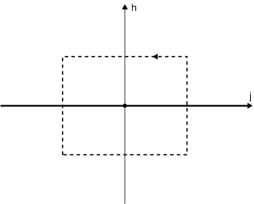
Figure 5. Same as Fig. 3 but for the m:-n resonant system.

Proposition 3.

The monodromy matrix of a $m:-n$ resonant system of the form (72) is given for $m$ and $n$ relatively prime and for a counterclockwise loop around the origin (see Fig. 4) by

(114) $$M=\left(\begin{array}[]{cc}1&0\\ -\frac{1}{mn}&1\end{array}\right)\ .$$

The proof of proposition 3 follows the same lines as for the resonance $1:-n$. As in Sec. 2.4, we consider the family of energy-momentum maps given by Eqs. (72) where $\pi_{1}$, $\pi_{3}$ and $J$ are given by Eqs. (68) with $m>1$. Some lemmas are required before the final proof.

Lemma 5.

The energy-momentum map $F$ of Eq. (72) has locally the bifurcation diagram of Fig. 5 in a neighborhood of the origin if $R$ is of the form

(115) $$R(\pi_{1},J)=(\pi_{1}+J)^{n^{\prime}}(\pi_{1}-J)^{m^{\prime}}\tilde{R}(\pi_{1},J)\ ,$$

where $n^{\prime}>\frac{n}{2}$, $m^{\prime}>\frac{m}{2}$. $\tilde{R}$ is a polynomial such that the two smallest real positive roots of $Q$ which are larger than $j$ are simple roots for $(h,j)\in\mathcal{R}_{reg}$. $Q$ is the following polynomial

(116) $$Q=(\pi_{1}+j)^{n}(\pi_{1}-j)^{m}-\big{(}h-R(\pi_{1},j)\big{)}^{2}\ .$$

The two roots are denoted $\pi_{1}^{-}$ and $\pi_{1}^{+}$.

Proof The proof is similar to the proof of lemma 2.$\Box$

Lemma 6.

The functions $\Theta$ and $\tau$ are defined for a point $(h,j)\in\mathcal{R}_{reg}$ by the following integrals

(119) $$\left\{\begin{array}[]{ll}\Theta(h,j)=\int_{\pi_{1}^{-}}^{\pi_{1}^{+}}[\frac{hu}{j+\pi_{1}}+\frac{hv}{\pi_{1}-j}]\frac{d\pi_{1}}{\sqrt{Q}}+\Theta_{0}(h,j)\\ \tau(h,j)=\frac{1}{mn}\int_{\pi_{1}^{-}}^{\pi_{1}^{+}}\frac{(j+\pi_{1})^{n-1}(\pi_{1}-j)^{m-1}}{\sqrt{Q}}d\pi_{1}\\ \end{array}\right.\ .$$

$\Theta_{0}$ is a function over $\mathcal{R}$ which is continuous on the line of singularities $C$. $u$ and $v$ are two integers such that $mu-nv=1$. $\tau$ is the first return time of the rescaled vector field $X=\frac{1}{(p_{1}^{2}+q_{1}^{2})^{n-1}(p_{2}^{2}+q_{2}^{2})^{m-1}}{X_{H}}$ defined such that $\tau$ has a non-zero finite limit on $C$.

Remark 4.

One can obtain the expression given by Eq. (85) corresponding to the case $1:-n$ as a special case of Eq. (119) with $u=1$ and $v=0$, which is a particular solution of $mu-nv=1$ for $m=1$.

Proof The determination of $\Theta$ is based on the dependence of the angle $\theta$ as a function of the coordinates $(p_{1},q_{1},p_{2},q_{2})$. To clarify this question, we introduce the canonical conjugate coordinates $(I_{1},\varphi_{1})$ and $(I_{2},\varphi_{2})$ which are defined as follows

(122) $$\left\{\begin{array}[]{ll}q_{k}=\sqrt{2I_{k}}\sin\varphi_{k}\\ p_{k}=\sqrt{2I_{k}}\cos\varphi_{k}\end{array}\right.\ .$$

Note that the polar coordinates $(I_{k},\varphi_{k})$ are only defined if $p_{k}^{2}+q_{k}^{2}>0$ [Arn89] which is not the case on the line $C$. By definition, the angles $\varphi_{1}$ and $\varphi_{2}$ vary in an interval of length $2\pi$. We look for a linear canonical transformation which transforms the two angles $\varphi_{1}$ and $\varphi_{2}$ into $\theta$ and $\psi$ where the angle $\theta$ is canonically conjugate to $J$. The angular dependence of $H$ in the variables $(I_{1},\varphi_{1},I_{2},\varphi_{2})$ is given by the term $\pi_{3}$ and is equal to $n\varphi_{1}+m\varphi_{2}$. We then set

(125) $$\left\{\begin{array}[]{ll}\theta=u\varphi_{1}+v\varphi_{2}\\ \psi=n\varphi_{1}+m\varphi_{2}\end{array}\right.\ ,$$

where $u$ and $v$ are integers such that $mu-nv=1$ which ensures that the determinant of the linear canonical transformation is 1 and that $\theta$ and $\psi$ are two angles varying in an interval of length $2\pi$. Since $m$ and $n$ are relatively prime, the Bezout theorem states that this equation has a solution ($u_{0}$,$v_{0}$). There are an infinite number of solutions which can be written ($u_{0}+kn$,$v_{0}+km$) with $k\in\mathbb{Z}$. We denote by $(u,v)$ one of these solutions. A choice of a couple $(u,v)$ is associated to a choice of a particular basis of the homology group.

The generating function $F_{2}$ of type 2 [Arn89] associated to the canonical transformation is given by

(126) $$F_{2}=(u\varphi_{1}+v\varphi_{2})\tilde{J}+(n\varphi_{1}+m\varphi_{2})\mathcal{I}\ ,$$

where $\tilde{J}$ and $\mathcal{I}$ are the momenta conjugated respectively to $\theta$ and $\psi$. From the definition of $F_{2}$, one deduces that

(129) $$\left\{\begin{array}[]{ll}\tilde{J}=mI_{1}-nI_{2}\\ \mathcal{I}=uI_{2}-vI_{1}\end{array}\right.\ ,$$

and that as expected $\tilde{J}=J$. We will drop the tilde in the rest of the proof.

The angle $\theta$ can therefore be written as

(130) $$\theta=u\arg(p_{1}+iq_{1})+v\arg(p_{2}+iq_{2})\ .$$

Differentiating Eq. (129) with respect to time and using the Hamilton equations, one obtains that

(131) $$\dot{\theta}=\frac{u\big{(}n\pi_{3}+\frac{\partial R}{\partial p_{1}}p_{1}+\frac{\partial R}{\partial q_{1}}q_{1}\big{)}}{q_{1}^{2}+p_{1}^{2}}+\frac{v\big{(}m\pi_{3}+\frac{\partial R}{\partial p_{2}}p_{2}+\frac{\partial R}{\partial q_{2}}q_{2}\big{)}}{q_{2}^{2}+p_{2}^{2}}\ ,$$

which leads to

(132) $$\dot{\theta}=\frac{u\big{(}nmh-nmR+m\frac{\partial R}{\partial p_{1}}p_{1}+m\frac{\partial R}{\partial q_{1}}q_{1}\big{)}}{j+\pi_{1}}+\frac{v\big{(}nmh-nmR+n\frac{\partial R}{\partial p_{2}}p_{2}+n\frac{\partial R}{\partial q_{2}}q_{2}\big{)}}{\pi_{1}-j}\ .$$

The last step consists in rewriting this integral as an integral in the reduced phase space $P_{j}$. The $R$-dependent part of $\Theta$ gives a continuous contribution on the line $C$ denoted $\Theta_{0}$. Since $\dot{\pi}_{1}=2mn\pi_{2}$, one finally obtains

(133) $$\Theta(h,j)=\int_{\pi_{1}^{-}}^{\pi_{1}^{+}}[\frac{hu}{j+\pi_{1}}+\frac{hv}{\pi_{1}-j}]\frac{d\pi_{1}}{\pi_{2}}+\Theta_{0}(h,j)\ .$$

For $\tau$ the proof is straightforward and similar to the one of lemma 3.$\Box$

Lemma 7.

The complex discriminant locus $\Delta$ near the origin is given by

(136) $$\Delta=\left\{\begin{array}[]{ll}h=0\\ h=\pm\sqrt{\frac{(-1)^{m}2^{m+n}m^{m}n^{n}j^{m+n}}{(m+n)^{m+n}}}\\ \end{array}\right.\ .$$

In the limit $h\to 0$, $j<0$ fixed, the polynomial $Q$ as a function of $x$ has n roots $x_{k}$ whose leading term is

(137) $$x_{k}=\frac{h^{2/n}}{(-2j)^{m/n}}e^{\frac{2i\pi k}{n}}\ .$$

with $k\in\{0,1,\cdots,n-1\}$, the other roots having a finite limit different from zero.

In the limit $h\to 0$, $j>0$ fixed, the polynomial $Q$ as a function of $x^{\prime}$ has m roots $x^{\prime}_{k}$ whose leading term is

(138) $$x^{\prime}_{k}=\frac{h^{2/m}}{(2j)^{n/m}}e^{\frac{2i\pi k}{m}}\ .$$

with $k\in\{0,1,\cdots,m-1\}$, the other roots having a finite limit different from zero.

Remark 5.

We notice that the case $j>0$ and $j<0$ give the same expressions but with $m$ and $n$ interchanged.

Proof Let us assume that $j<0$. As for the $1:-n$ resonance, we calculate the complex discriminant locus of $Q$ near the origin as a function of $x$. The construction of the Newton polyhedron gives the principal part $Q_{N}$ of $Q$

(139) $$Q_{N}(x)=(x-2j)^{m}x^{n}-h^{2}\ .$$

Simple algebra leads to the discriminant locus $\Delta$.

In the limit $h\to 0$, $j<0$ fixed, the construction of the Newton polygon of $Q$ leads to the following equation for the roots of the principal part of $Q$

(140) $$(-2j)^{m}x^{n}=h^{2}\ ,$$

and to the $n$ roots $x_{k}$ of Eq. (137). Exchanging the role of $m$ and $n$ and taking $j>0$, a similar proof gives the roots of Eq. (138).$\Box$

Having established lemmas 5, 6 and 7 required, we can pass to the proof of proposition 3.

Proof Since the line $C$ is crossed two times by the loop $\Gamma$, the monodromy matrix $M$ has two contributions denoted $M_{-}$ for $j<0$ and $M_{+}$ for $j>0$. We first consider the case $j<0$. The case $j>0$ will be deduced from the calculation for $j<0$ by exchanging the role of $m$ and $n$. The calculation is based on the analysis of the roots of the polynomial $Q$. $Q$ has $N$ roots denoted $x_{i}$ with $i\in\{0,1,\cdots N-1\}$. The roots $x_{n},\cdots x_{N-1}$ are of order 1. A simple analysis of the polynomial $Q$ leads to the following relations

(144) $$\left\{\begin{array}[]{lll}\prod_{i=0}^{N-1}x_{i}=h^{2}(-1)^{N+1}\\ \prod_{i=0}^{n-1}x_{i}=\frac{h^{2}}{(-2j)^{m}}(-1)^{n-1}\\ \prod_{i=n}^{N-1}x_{i}=(-1)^{N-n+m}(-2j)^{m}\\ \end{array}\right.\ .$$

Following the same steps as in the proof for the resonance $1:-n$, one arrives to

(145) $$\Theta(h,j)-\Theta_{0}(h,j)\sim uh\int_{\frac{|h|^{2/n}}{(-2j)^{m/n}}}^{k}\frac{dx}{x\sqrt{(-2j)^{m}(x^{n}-\frac{h^{2}}{(-2j)^{m}})\times 1}}\ ,$$

where $\frac{|h|^{2/n}}{(-2j)^{m/n}}\ll k\ll 1$. For $h>0$, Eq. (145) simplifies into

(146) $$\Theta(h,j)-\Theta_{0}(h,j)\sim u\int_{1}^{+\infty}\frac{dx}{x\sqrt{x^{n}-1}}\ .$$

We finally obtain that

(147) $$\lim_{h\to 0^{\pm},j<0}=\Theta(h,j)-\Theta_{0}(h,j)=\pm u\frac{\pi}{n}\ .$$

A similar proof leads to

(148) $$\lim_{h\to 0^{\pm},j>0}=\Theta(h,j)-\Theta_{0}(h,j)=\pm v\frac{\pi}{m}\ .$$

The calculation of $\tau$ uses the same arguments and shows that $\tau$ is continuous on $C$.

One then deduces that the matrices $M_{-}$ and $M_{+}$ are respectively given by

(151) $$M_{-}=\left(\begin{array}[]{cc}1&0\\ -\frac{u}{n}&1\end{array}\right)\ ,$$

and

(154) $$M_{+}=\left(\begin{array}[]{cc}1&0\\ \frac{v}{m}&1\end{array}\right)\ ,$$

where we have taken into account for $M_{+}$ the fact that the line $C$ is crossed from $h<0$ to $h>0$. The total monodromy matrix is given by the product of the matrices $M_{-}$ and $M_{+}$

(161) $$M=\left(\begin{array}[]{cc}1&0\\ -\frac{u}{n}&1\end{array}\right)\left(\begin{array}[]{cc}1&0\\ \frac{v}{m}&1\end{array}\right)=\left(\begin{array}[]{cc}1&0\\ -\frac{1}{mn}&1\end{array}\right)\ ,$$

where the relation $mu-nv=1$ has been used.$\Box$

3. Extension to the complex domain

3.1. Idea of the method

In this section, we reformulate the notion of fractional hamiltonian monodromy by deforming the loop $\Gamma$ close to the line $C$, such that it bypasses the line $C$ through the complex domain. The starting point of the complex approach is given by the expressions of the functions $\Theta$ and $\tau$ as real one-dimensional integrals (see for instance lemma 1, Eqs. (26) and (27) for the 1:-2 resonance case). If we consider the complexified variables $h$, $j$ and $\pi_{1}$ then $\Theta(h,j)$ and $\tau(h,j)$ can be interpreted as complex integrals on a line of the complex plane $\pi_{1}$. Furthermore, these two functions can be rewritten as integrals of rational 1-forms over a cycle $\delta$ on the Riemann surface defined by $\pi_{2}^{2}=Q(\pi_{1})$. This allows the use of topological properties of the Riemann surfaces.

More precisely, we first introduce a Riemann surface constructed from the energy-momentum map $F$ and we determine the Gauss-Manin connection of a complex semi-circle $\Gamma_{C}$ bypassing the line $C$ of singularities. As explained below, we can then construct the extension to the complex domain of the functions $\Theta$ and $\tau$ along $\Gamma_{C}$. The monodromy matrix is determined as in the real approach by the variation of the functions $\Theta$ and $\tau$ along a loop $\Gamma$ around the origin. The regularizations of the functions $\Theta$ and $\tau$ to cross the line $C$ are replaced by their continuations along $\Gamma_{C}$. We obtain the fractional monodromy matrix by letting the radius of the complex semi-circle $\Gamma_{C}$ tend to 0.

3.2. Extension to the complex domain of the 1:-2 resonant system

Remark 6.

All that has been established in Sec. 2.1 for the real approach can be done exactly in the same way for the complexified phase space $T^{*}\mathbb{C}^{2}$ where $(J,\pi_{1},\pi_{2},\pi_{3})\in\mathbb{C}^{4}$, except for the fact that there is no restriction on the values of $J$ and $\pi_{1}$. The quotient is taken to be $\mathbb{C}^{*}\sim S^{1}\times\mathbb{R}^{*}$. The reduction in the complex approach is described in appendix C. The manifold $\mathbb{C}^{4}/S^{1}\times\mathbb{R}^{*}$ has real dimension 6.

We begin by recalling some of the basic elements of the theory of complex algebraic curves which will be used throughout this section (see [Kir93] for a comprehensive introduction).

Let $P:\mathbb{C}^{2}\to\mathbb{C}$ be a polynomial function. The fibers $P^{-1}(z)$ are complex algebraic curves (hence two-dimensional real surfaces). There exists a finite set $\Sigma\subset\mathbb{C}$ (essentially critical values of $P$) such that all fibers $P^{-1}(z)$, $z\in\mathbb{C}\setminus\Sigma$, look alike. Moreover, the mapping $P:\mathbb{C}^{2}\setminus(P^{-1}(\Sigma))\to\mathbb{C}\setminus\Sigma$ is a locally trivial fibration. Hence, given any path $\gamma:[z_{0},z_{1}]\to\mathbb{C}\setminus\Sigma$, one can identify the fibers $P^{-1}(\gamma(z_{0}))$ and $P^{-1}(\gamma(z_{1}))$. This identification is not unique but induces a unique identification between the homology groups of the two fibers. For $z_{0}\in\mathbb{C}\setminus\Sigma$, a cycle $\delta(z_{0})\in H_{1}(P^{-1}(z_{0}))$ can be transported along any path $\gamma$ in $\mathbb{C}\setminus\Sigma$ starting at $z_{0}$ giving thus a family of cycles $\delta(z)$. The transport depends only on the homotopy class of the path $\gamma$ in $\mathbb{C}\setminus\Sigma$. This is the classical Gauss-Manin connection [AGZV88, Zol06]. The Gauss-Manin monodromy is defined from the Gauss-Manin connection as an automorphism of the homology group $H_{1}$ for a loop in $\mathbb{C}\setminus\Sigma$.

For the 1:-2 resonance (see Sec. 2.2), the energy-momentum map of Eqs. (3) can be treated in the formalism of complex algebraic curves even if the situation is more complicated than described above. The difficulty here lies in the fact that the fibration is defined only implicitly by

(162) $$F^{\mathbb{C}}:=\pi_{2}^{2}-[(\pi_{1}-j)(\pi_{1}+j)^{2}-\big{(}h-\varepsilon(\pi_{1}^{2}-j^{2})\big{)}^{2}]=0\ ,$$

i.e. $\pi_{2}^{2}=Q(\pi_{1},j,h)$.

For fixed generic values of $(h,j)$, Eq. (162) defines a torus from which two points at infinity have been deleted. The corresponding complex algebraic curve is schematically represented in Fig. 6. This representation can be understood by solving Eq. (162) with respect to $\pi_{2}$. Generically, there are four values of $\pi_{1}$ for which $Q(\pi_{1},j,h)=0$, giving each a single solution for $\pi_{2}=0$. These points are the ramification points of the complex algebraic curve. For all other points $\pi_{1}$, there are two solutions $\pi_{2}$ of Eq. (162) represented by the two leaves in Fig. 6.

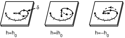
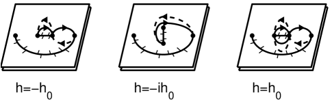
Figure 6. Transport of the cycle $\delta$ along a loop around the line $C$. The loop is an arc of a circle of radius $h_{0}>0$. The large solid lines represent arbitrary branch cuts of the Riemann surfaces and the full dots ramification points (see text). The parts in solid and dashed lines of the loop respectively lie in the upper and lower leaves of the Riemann surface.

We denote by $F^{\mathbb{C}}_{(j,h)}$ the set of points $(\pi_{1},\pi_{2})\in\mathbb{C}^{2}$ such that $(\pi_{1},\pi_{2},j,h)$ verify Eq. (162). Note that for two different values $(h,j)\not=(h^{\prime},j^{\prime})$ the fibers $F^{\mathbb{C}}_{(j,h)}$ and $F^{\mathbb{C}}_{(j^{\prime},h^{\prime})}$ intersect. Nevertheless, it is possible to generalize the Gauss-Manin connection to this case. Consider for that the mapping $G:\mathbb{C}^{4}\to\mathbb{C}^{3}$, given by

(163) $$G(\pi_{1},\pi_{2},h,j)=(\pi_{2}^{2}-Q(\pi_{1},h,j),h,j)\ .$$

The mapping $G$ defines a fibration on the complement $\mathbb{C}^{3}\setminus\Sigma$ of the set $\Sigma\in\mathbb{C}^{3}$ where its rank is not maximal. We use here the Ehresmann fibration theorem [Wolf64]. We take as basis of our fibration denoted $\mathcal{B}\in\mathbb{C}^{2}$ the set $(\{0\}\times\mathbb{C}^{2})\cap(\mathbb{C}^{3}\setminus\Sigma)$ which is viewed as a set in the $(h,j)$-space $\mathbb{C}^{2}$. As in the real approach, we introduce the variable $x=j+\pi_{1}$ and we set $y=\pi_{2}$. The singular locus of the fibration is the set of points $(h,j)\in\mathbb{C}^{2}$ where the polynomial $Q$ has multiple complex roots. This set is given by Eq. (35) and is displayed for $j\in\mathbb{R}$ in Fig. 8. We notice that for $(h,j)=(0,0)$ the fibration is singular and that the singularity $(x=0,y=0)$ is not of Morse type.

In the reduced phase space $P_{j}$, the original real torus projects to a cycle $\delta(h,j)$ delimited by $\pi_{1}^{-}$ and $\pi_{1}^{+}$ (see for instance Fig. 4). $\pi_{1}^{-}$ and $\pi_{1}^{+}$ are the two largest real roots of the polynomial $Q$ as a function of $\pi_{1}$. Returning back to the Riemann surface and following notations of Eqs. (45), the roots of $Q$, which are simple ramification points of the Riemann surface, are denoted $x_{k}$ ($k=1,\cdots 4$). One can introduce cuts along the segment $x_{2}x_{3}$ and along a simple curve joining $x_{1}$ and $x_{4}$ and avoiding the segment $x_{2}x_{3}$. For $(h,j)\in\mathcal{R}_{reg}$, the cycle $\delta(h,j)$ is represented by the real oval between the two largest real ramification points which correspond respectively to $j+\pi_{1}^{-}$ and $j+\pi_{1}^{+}$. To be coherent with the real approach, this cycle is oriented from $x=j+\pi_{1}^{-}$ to $x=j+\pi_{1}^{+}$ in the upper leaf and from $x=j+\pi_{1}^{+}$ to $x=j+\pi_{1}^{-}$ in the lower one. All these notations are displayed in Fig. 6.

3.3. Computation of fractional monodromy from the Gauss-Manin monodromy

We pursue in this section the construction for the 1:-2 resonant system to arrive to the computation of fractional monodromy at the end of the section. Let $\Gamma$ be a loop around the origin. We recall that the computation of the monodromy matrix associated to $\Gamma$ is based on the difference of the values of the functions $\Theta$ and $\tau$ at each side of $C$ as $h$ goes to 0. The goal here is to compute the variations of these functions using their extensions to the complex domain near $C$.

Definition 2.

Starting with the result of lemma 1, we introduce the complex continuation of the functions $\Theta$ and $\tau$ defined by

(166) $$\left\{\begin{array}[]{ll}\Theta(h,j)=\frac{h}{2i\varepsilon}\int_{\delta(h,j)}\frac{dx}{xy}\\ \tau(h,j)=\frac{1}{4i\varepsilon}\int_{\delta(h,j)}\frac{xdx}{y}\end{array}\right.\ ,$$

where $(h,j)\in\mathcal{B}$ and $y^{2}=(x-x_{1})(x-x_{2})(x-x_{3})(x-x_{4})$. The positive and negative determinations of the square root $y$ have been chosen respectively for the upper and the lower leaves of the Riemann surface. We have added a factor $\frac{1}{2}$ in the definition of $\Theta$ and $\tau$ to coincide with the real case.

We locally deform in a neighborhood of the line $C$ the loop $\Gamma$. We denote by $\Gamma_{C}$ this complex deformation and by $\Gamma_{R}$ the rest of the loop. $\Gamma$, $\Gamma_{C}$ and $\Gamma_{R}$ are represented in Figs. 8 and 9.

Remark 7.

In this work, we have considered deformations of the real loop in the half-plane $\Im[h]>0$ but they could be equivalently done in the half-plane $\Im[h]<0$.

The bypass $\Gamma_{C}(h_{0})$ is a semi-circle of radius $h_{0}$ in a plane with $j_{0}<0$ fixed around the line $C$. The corresponding real path completing $\Gamma_{C}(h_{0})$ is denoted $\Gamma_{R}(h_{0})$. From Eq. (35) and for a small $j_{0}$, one deduces that if $h_{0}<\sqrt{\frac{-32}{27}j_{0}^{3}}$ then $x_{2}$ and $x_{3}$ exchange their positions along $\Gamma_{C}(h_{0})$ whereas if $h_{0}>\sqrt{\frac{-32}{27}j_{0}^{3}}$ then 3 ramification points of the Riemann surface ($x_{1}$, $x_{2}$ and $x_{3}$) move and exchange their positions. The change of the ramification points is displayed in Fig. 10. It can also be deduced from the asymptotic expansions of the roots of $Q$ [see Eqs. (45)]. This can be seen by parameterizing the loop $\Gamma_{C}(h_{0})$ as

(169) $$\left\{\begin{array}[]{ll}h=h_{0}e^{it}\\ j=j_{0}\end{array}\right.\ .$$

where $t\in[0,\pi]$. There is thus a qualitative difference of the result depending on the value of $h_{0}$. $h_{0}$ must be chosen sufficiently small to be in the first case since for each fixed $j_{0}$ we are interested in the limit $h_{0}\to 0$.

The family of cycles $\delta(h,j)$ can be obtained by transport of the cycle $\delta(h_{0},j_{0})$ along $\Gamma_{R}$. Examining Fig. 10, one sees that the lines of singularities crossed by $\Gamma_{R}$ have no incidence on the ramification points defining the cycle $\delta$. The parallel transport of $\delta$ along $\Gamma_{C}(h_{0})$ is given by the change of the ramification points along $\Gamma_{C}(h_{0})$. From the Picard-Lefshetz theory [Zol06, AGZV88] (see Figs. 6), one can show that the cycle $\delta(h_{0},j_{0})$ when transported along the bypass $\Gamma_{C}(h_{0})$ is transformed into $\delta(-h_{0},j_{0})+\delta_{0}(-h_{0},j_{0})$ where $\delta_{0}$ is a vanishing cycle around the ramification points $x_{2}$ and $x_{3}$ of the fiber $F^{\mathbb{C}}_{(-h_{0},j_{0})}$. $x_{2}$ and $x_{3}$ are defined by Eqs. (50). For the position of the cuts of Figs. 6, the cycle $\delta_{0}(-h_{0},j_{0})$ is composed of a path from $x_{3}$ to $x_{2}$ on the upper leaf followed by the lift of the same path to the lower leaf run in the opposite direction. The vanishing cycles $\delta_{0}$ and $\delta_{1}$ are represented in Fig. 7. The cycle $\delta_{1}$ will be used in lemma 8. Note the different choices of cuts for the Riemann surface between Figs. 6 and Fig. 7.

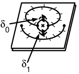
Figure 7. Definition of the cycle $\delta_{0}$ and $\delta_{1}$ for the 1:-2 resonance. The position of the pole of $\Theta$ is represented by a cross.

Hence, an abelian integral $I(h_{0},j_{0})=\int_{\delta(h_{0},j_{0})}\omega$ becomes after going once around the semi-circle $\Gamma_{C}(h_{0})$ the sum $I(-h_{0},j_{0})+\int_{\delta_{0}(-h_{0},j_{0})}\omega$ which gives the variation of the function $I$ over $\Gamma_{C}(h_{0})$. This latter remark can be applied to the functions $\Theta$ and $\tau$. However, due to the presence of a pole at $x=0$ for the function $\Theta$, the cycle $\delta_{0}$ has to be positioned with respect to $x=0$. The counterclockwise turning of the ramification points $x_{2}$ and $x_{3}$ implies that the cycle $\delta_{0}$ avoids the singularity $x=0$ from above.

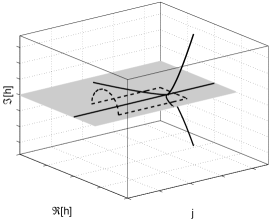
Figure 8. Complex discriminant locus $\Delta$ (solid lines) of the energy-momentum map of Eq. (3) for $j\in\mathbb{R}$ and $h\in\mathbb{C}$. The grey plane corresponds to the real bifurcation diagram. The dashed lines represent the loop $\Gamma$ locally deformed near $C$ to the complex domain. The arc of circle is in a complex $h-plane$ with $j$ fixed.

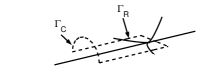
Figure 9. Decomposition of the loop $\Gamma$ into the paths $\Gamma_{C}$ and $\Gamma_{R}$.

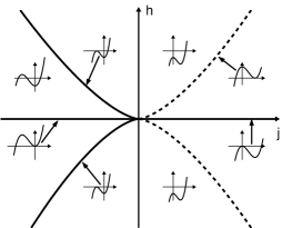
Figure 10. Schematic representation of three of the roots of the polynomial $Q$ as a function of $h$ and $j$. These roots are the roots of the principal part $Q_{N}$ of $Q$ defined by Eq. (32). The polynomial $Q$ has another root larger in module which is not represented here as it undergoes no bifurcation. The small inserts depict the graph of $Q_{N}$ as a function of $x$ for different values of $h$ and $j$. The position of the inserts gives the corresponding values of $h$ and $j$. The solid and dashed lines are lines of singularities of $\Delta$. The dashed lines do not belong to the real bifurcation diagram (see Fig. 8).

From the analysis of the behavior of the cycle $\delta$ along $\Gamma$, we can determine the variations of the functions $\Theta$ and $\tau$ along this loop. These variations are denoted $\Delta\Theta_{\Gamma}(h_{0})$ and $\Delta\tau_{\Gamma}(h_{0})$ and defined as follows

Definition 3.

For the energy-momentum map of Eq. (3), $\Delta\Theta_{\Gamma}(h_{0})$ and $\Delta\tau_{\Gamma}(h_{0})$ are given in the complex approach by

(172) $$\left\{\begin{array}[]{ll}\Delta\Theta_{\Gamma}(h_{0})=\Delta\Theta_{\Gamma_{C}}(h_{0})+\Delta\Theta_{\Gamma_{R}}(h_{0})\\ \Delta\tau_{\Gamma}(h_{0})=\Delta\tau_{\Gamma_{C}}(h_{0})+\Delta\tau_{\Gamma_{R}}(h_{0})\end{array}\right.\ .$$

A simple calculation allows to simplify the expressions of $\Delta\Theta_{\Gamma}(h_{0})$ and $\Delta\tau_{\Gamma}(h_{0})$. Since

(173) $$\Delta\Theta_{R}(h_{0})=\frac{h_{0}}{2i\varepsilon}\int_{\delta(h_{0},j_{0})}\frac{dx}{xy}-\frac{-h_{0}}{2i\varepsilon}\int_{\delta(-h_{0},j_{0})}\frac{dx}{xy}\ ,$$

and

(174) $$\Delta\Theta_{C}(h_{0})=\frac{-h_{0}}{2i\varepsilon}\int_{\delta(-h_{0},j_{0})}\frac{dx}{xy}+\frac{-h_{0}}{2i\varepsilon}\int_{\delta_{0}(-h_{0},j_{0})}\frac{dx}{xy}-\frac{h_{0}}{2i\varepsilon}\int_{\delta(h_{0},j_{0})}\frac{dx}{xy}\ ,$$

one deduces for $j_{0}<0$ fixed that

(177) $$\left\{\begin{array}[]{ll}\Delta\Theta_{\Gamma}(h_{0})=-\frac{h_{0}}{2i\varepsilon}\int_{\delta_{0}(-h_{0},j_{0})}\frac{dx}{xy}\\ \Delta\tau_{\Gamma}(h_{0})=\frac{1}{4i\varepsilon}\int_{\delta_{0}(-h_{0},j_{0})}\frac{xdx}{y}\end{array}\right.\ .$$

We introduce for the function $\Theta$ the following quantities

(181) $$\left\{\begin{array}[]{lll}\Delta\Theta_{\Gamma}=\lim_{h_{0}\to 0}\Delta\Theta_{\Gamma}(h_{0})\\ \Delta\Theta_{\Gamma_{C}}=\lim_{h_{0}\to 0}\Delta\Theta_{\Gamma_{C}}(h_{0})\\ \Delta\Theta_{\Gamma_{R}}=\lim_{h_{0}\to 0}\Delta\Theta_{\Gamma_{R}}(h_{0})\end{array}\right.\ ,$$

and the same for $\tau$.

Different results have to be established before computing the monodromy matrix. The variation of $\Theta$ around $C$ can be viewed as a residue.

Lemma 8.

The sum of the integrals of the 1-form $\frac{h_{0}}{2i\varepsilon}\frac{dx}{xy}$ over $\delta_{0}$ and $\delta_{1}$ is independent of $h_{0}$ and $j_{0}$ and equal to

(182) $$\frac{h_{0}}{2i\varepsilon}\int_{\delta_{0}(h_{0},j_{0})}\frac{dx}{xy}+\frac{h_{0}}{2i\varepsilon}\int_{\delta_{1}(h_{0},j_{0})}\frac{dx}{xy}=2\pi\ .$$

In this equation, $h_{0}$ is taken sufficiently small and $j_{0}<0$.

Proof We use the notations of Fig. 7. The union of $\delta_{0}$ and $\delta_{1}$ corresponds to two loops around the pole $x=0$ lying respectively in the upper and the lower leaves of the Riemann surface. The orientation of these two loops is on the lower leaf the opposite to the one on the upper leaf. The same applies to the determination of the square root $y$ for the two leaves of the Riemann surface. Hence, the sum of the left hand-side of Eq. (182) is given by two times the residue of the 1-form $\frac{dx}{xy}$ at $x=0$. One deduces that

(183) $$\frac{h_{0}}{2i\varepsilon}\int_{\delta_{0}(h_{0},j_{0})}\frac{dx}{xy}+\frac{h_{0}}{2i\varepsilon}\int_{\delta_{1}(h_{0},j_{0})}\frac{dx}{xy}=\frac{h_{0}}{2i\varepsilon}4\pi i\textrm{Res}(\frac{1}{xy},x=0)\ .$$

Simple algebra leads to

(184) $$\textrm{Res}(\frac{1}{xy},x=0)=\frac{\varepsilon}{h_{0}}\ ,$$

which completes the proof.$\Box$

Lemma 9.

The variations of the functions $\Theta$ and $\tau$ along $\Gamma$ are

(187) $$\left\{\begin{array}[]{ll}\Delta\Theta_{\Gamma}=\pi\\ \Delta\tau_{\Gamma}=0\end{array}\right.\ .$$

Proof We use Eqs. (177) and we calculate these two quantities in the limit $h_{0}\to 0$ and $j_{0}<0$ fixed. The asymptotic expansion of the roots $x_{i}$ for $h\to 0$ and $j<0$ fixed is given by Eqs. (50) [see Ref. [ECS07] for the explicit computation].

We begin by the computation of $\Delta\Theta_{\Gamma}$. We first notice that $x_{2}$ and $x_{3}$ are real. $\delta_{0}$ can thus be viewed as a real loop which is locally deformed in a neighborhood of $x=0$ to avoid the pole in $x=0$. Since the path $\delta_{0}$ is oriented in the opposite direction and the sign of $y$ is the opposite in the lower leaf with respect to the upper leaf, it is straightforward to see that the contributions of the upper and lower leaves of the Riemann surface coincide. $\Delta\Theta_{\Gamma}$ can be written as follows

(188) $$\Delta\Theta_{\Gamma}=\lim_{h_{0}\to 0}\big{[}PV\frac{-h_{0}}{i\varepsilon}\int_{x_{3}}^{x_{2}}\frac{dx}{xy}+\frac{h_{0}}{i\varepsilon}\frac{1}{2}2\pi i\textrm{Res}(\frac{1}{xy},x=0)\big{]}\ ,$$

where $PV$ denotes the principal value of the integral. The introduction of the principal value is due to the presence of the pole at $x=0$. The residue is calculated with the positive determination of the square root $y$. The factor $\frac{-1}{2}$ in front of the residue corresponds to the fact that the integral is taken on a semi-circle which is oriented in a clockwise manner. The contribution of the residue term to $\Delta\Theta_{\Gamma}$ is equal to $\pi$. Following Ref. [ECS07], the computation of the principal value term can be done by using elliptic integrals. It can be shown that this term is zero.

Using the same arguments, we can deduce that $\Delta\tau_{\Gamma}=0$ since $\tau$ has no singularity along the real segment $x_{2}x_{3}$.$\Box$ In the limit $h_{0}\to 0$, $\delta_{0}$ and $\delta_{1}$ play a symmetrical role for $\Theta$. More precisely, we have

Corollary 1.

The integrals of the 1-form $\frac{h_{0}}{2i\varepsilon}\frac{dx}{xy}$ over $\delta_{0}$ and $\delta_{1}$ are given by

(189) $$\lim_{h_{0}\to 0}\frac{h_{0}}{2i\varepsilon}\int_{\delta_{0}(h_{0},j_{0})}\frac{dx}{xy}=\lim_{h_{0}\to 0}\frac{h_{0}}{2i\varepsilon}\int_{\delta_{1}(h_{0},j_{0})}\frac{dx}{xy}=\pi\ .$$

Proof The proof of lemma 9 has already shown that

(190) $$\lim_{h_{0}\to 0}\frac{h_{0}}{2i\varepsilon}\int_{\delta_{0}(h_{0},j_{0})}\frac{dx}{xy}=\pi\ .$$

We conclude for $\delta_{1}$ by using lemma 8.$\Box$

Remark 8.

We remark that the complex continuations of the functions $\Theta$ and $\tau$ along $\Gamma_{C}$ have replaced the regularizations of these functions in the real approach. The semi-circle $\Gamma_{C}$ is taken to be asymptotic in order for $\Delta\Theta_{\Gamma}$ and $\Delta\tau_{\Gamma}$ to be independent of $h$ and $j$ and to recover the topological character of fractional monodromy. In contrast, if we consider a loop around the line $C$ then the variation of $\Theta$ along this loop is topological as it is calculated from a residue (see lemma 8).

From lemma 9, we can finally conclude by the following proposition.

Proposition 4.

The monodromy matrix $M$ for the loop $\Gamma$ is given by

(193) $$M=\left(\begin{array}[]{cc}1&0\\ -\frac{1}{2}&1\end{array}\right)\ ,$$

Proof We use lemma 9 and the fact that the monodromy matrix is determined by the variations $\Delta\Theta_{\Gamma}$ and $\Delta\tau_{\Gamma}$.$\Box$

Remark 9.

In the computation of lemma 9, we have taken arbitrary $j$, which shows the topological character of the definition of fractional monodromy.

We note that the real and the complex approach can be related by the following corollary.

Corollary 2.

$\Delta\Theta_{C}=0$ and hence $\Delta\Theta_{R}=\Delta\Theta_{\Gamma}$

Proof We apply the Jordan’s lemma to show that $\Delta\Theta_{C}=0$.$\Box$ The monodromy matrix in the real approach (resp. complex approach) is given by $\Delta\Theta_{R}$ and $\Delta\tau_{R}$ (resp. $\Delta\Theta_{\Gamma}$ and $\Delta\tau_{\Gamma}$). The corollary 2 shows that these two approaches are equivalent.

3.4. Generalization to $1:-n$ resonance

All the arguments used for constructing the extension to the complex domain of 1:-2 resonant systems can be generalized to $1:-n$ and $m:-n$ resonant systems. As for the real approach, we consider the family $\mathcal{F}$ of energy-momentum maps introduced in Eqs. (72).

The Riemann surface is defined from the relation deduced from Eqs. (69) and (72)

(194) $$y^{2}=x^{n}(x-2j)-[h-R(x-j,j)]^{2}\ .$$

The discriminant locus $\Delta$ of these systems is given locally by Eq. (96). Note that this locus is qualitatively different according to the parity of $n$. More precisely, the real lines of singularities for $n$ odd become purely imaginary for $n$ even. This does not change the discussion of this section. Following the preceding case, we consider a loop $\Gamma$ around the origin which decomposes into a complex semi-circle $\Gamma_{C}$ around the line $C$ and a real path $\Gamma_{R}$. Along $\Gamma_{C}$, one sees by using the expansion of the roots of $Q$ (lemma 4) that for $j<0$, $n$ roots in the variable $x$ turn asymptotically around the origin by an angle $\frac{2\pi}{n}$. The other roots stay fixed to first order in $h$. Fig. 11 illustrates this point for the resonance 1:-3. Note that only the principal part of the roots are exactly exchanged among each other.

Figure 11. Evolution of three of the roots (see text) of the polynomial $Q$ from the resonance 1:-3 and for a complex semi-circle going for $h_{0}>0$ to $-h_{0}<0$ ($j_{0}<0$ fixed). Numerical values are taken to be $h_{0}=0.005$ and $j_{0}=-1$. The radius of the semi-circle is $h_{0}$. The energy-momentum map is given by Eqs. (75). The full and open dots represent respectively the roots for the starting and the ending points of the path. The dashed line is a circle of radius $\frac{h_{0}^{2/3}}{(-2j)^{1/3}}$ which corresponds to the leading term of the expansion of the roots as $h_{0}\to 0$.

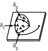
Figure 12. Definition of the cycles $\delta_{0}$, $\delta_{1}$ and $\delta_{2}$ for the 1:-3 resonance. The cross indicates the position of the pole of $\Theta$.

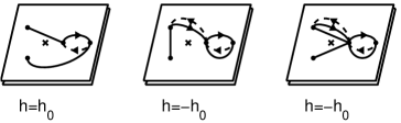
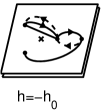
Figure 13. Transport of the cycle $\delta$ along a semi-circle around the line $C$. The radius of the semi-circle is $h_{0}$. The last three figures are equivalent but with different cuts. The cross indicates the position of the pole of $\Theta$.

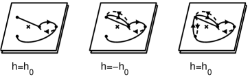
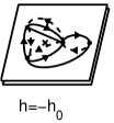
Figure 14. Same as Fig. 13 but for 3 semi-circles around the line $C$.

Following the change of the ramification points, we can transport the cycle $\delta$ along $\Gamma_{C}$. $\delta(h,j)$ is a real oval between $x_{0}$ and the ramification point of the Riemann surface associated to $\pi_{1}^{+}$ denoted $x_{n}$. This cycle is oriented from $x_{0}$ to $x_{n}$ in the upper leaf and from $x_{n}$ to $x_{0}$ in the lower one. Figures 13 and 14 display the transport of $\delta$. Not all the ramification points are represented in Figs. 13 and 14. The position of the cuts is arbitrary but indicates on which leaf of the Riemann surface a path lies. We can compare two Riemann surfaces if the cuts of the two surfaces are the same. Since for the 1:-n resonance the cuts move after a semi-circle, one has to modify the cuts to recover the initial choice of cuts. An example of this deformation is given in Figs. 13.

We see that after the semi-circle $\Gamma_{C}(h_{0})$ around $C$, $\delta(h_{0},j_{0})$ is transformed into $\delta(-h_{0},j_{0})+\delta_{0}(-h_{0},j_{0})$. $\delta_{0}$ is composed of a path from $x_{0}$ to $x_{n-1}$ in the upper leaf and of the lift of the same path in the lower leaf but run in the opposite direction.

Definition 4.

We define the complex extension of the functions $\Theta$ and $\tau$ as

(195) $$\Theta(h,j)=\frac{h}{2}\int_{\delta(h,j)}\frac{dx}{xy}+\Theta_{0}(h,j)\ ,$$

where the positive determination of the square root $y$ is associated to the upper leaf and

(196) $$\tau(h,j)=\frac{1}{2n}\int_{\delta(h,j)}\frac{x^{n-1}dx}{y}\ .$$

$\Theta_{0}$ is the complex extension of the real function $\Theta_{0}$ introduced in Eq. (91). $\Theta_{0}$ has a trivial contribution to the monodromy matrix.

We define the variations $\Delta\Theta_{\Gamma}(h_{0})$ and $\Delta\tau_{\Gamma}(h_{0})$ of the functions $\Theta$ and $\tau$ along $\Gamma$ as in the definition 3 for the 1:-2 resonance. These variations are given by integrals over the cycle $\delta_{0}$. $\Delta\Theta_{\Gamma}$ and $\Delta\tau_{\Gamma}$ denote the limits of these variations as $h_{0}\to 0$. They are given by

(199) $$\left\{\begin{array}[]{ll}\Delta\Theta_{\Gamma}=\lim_{h_{0}\to 0}\Delta\Theta_{\Gamma}(h_{0})\\ \Delta\tau_{\Gamma}=\lim_{h_{0}\to 0}\Delta\tau_{\Gamma}(h_{0})\end{array}\right.\ .$$

Equivalent lemmas to lemmas 8 and 9 for the $1:-2$ resonance can be established for the $1:-n$ resonance. We only state the final result.

Proposition 5.

The monodromy matrix associated to the loop $\Gamma$ is equal to

(202) $$M=\left(\begin{array}[]{cc}1&0\\ -\frac{1}{n}&1\end{array}\right)\ .$$

Proof We compute the different integrals in the limit $h_{0}\to 0$ with $j_{0}<0$ fixed. $\Delta\Theta_{\Gamma}(h_{0})$ can be written as

(203) $$\Delta\Theta_{\Gamma}(h_{0})=\frac{-h_{0}}{2}\int_{\delta_{0}(-h_{0},j_{0})}\frac{dx}{xy}\ ,$$

where $\delta_{0}$ is the cycle between $x_{0}$ and $x_{n-1}$ which is oriented from $x_{0}$ to $x_{n-1}$ in the upper leaf and inversely in the lower leaf. In the limit $h_{0}\to 0$, one deduces that

(204) $$\Delta\Theta_{\Gamma}=\lim_{h_{0}\to 0}h_{0}\int^{x_{0}}_{x_{n-1}}\frac{dx}{x\sqrt{\prod_{k=0}^{N-1}(x-x_{k})}}\ ,$$

where the integral is taken along an arc of a circle from $x_{n-1}$ to $x_{0}$ of radius $\frac{h_{0}^{2/n}}{(-2j)^{1/n}}$. Using the change of variables $x=\frac{h_{0}^{2/n}}{(-2j)^{1/n}}e^{i\chi}$, we obtain

(205) $$\Delta\Theta_{\Gamma}=\int_{0}^{2\pi/n}\frac{d\chi}{\sqrt{\prod_{k=0}^{n-1}(e^{i\chi}-e^{2i\pi k/n})}}\ .$$

It is straightforward to check that the integrand is not modified by the translation $\chi^{\prime}=\chi+\frac{2\pi}{n}$. One then deduces that

(206) $$\Delta\Theta_{\Gamma}=\lim_{h_{0}\to 0}-\frac{1}{n}\textrm{Res}[\frac{-h_{0}}{x\sqrt{\prod_{k=0}^{N-1}(x-x_{k})}},x=0]\ .$$

Simple algebra finally gives

(207) $$\Delta\Theta_{\Gamma}=\frac{2\pi}{n}\ .$$

Similar arguments show that $\Delta\tau_{\Gamma}=0$. We finally construct the monodromy matrix from the variations of $\Theta$ and $\tau$ along $\Gamma$. $\Box$

We finish this section by presenting a complementary computation of fractional hamiltonian monodromy in the complex approach. The idea is here to use direct asymptotic computations to determine $\Delta\Theta_{\Gamma}$.

Lemma 10.

For $j<0$ fixed and $|h|\to 0$, we have the following asymptotic behavior

(208) $$\Theta(h,j)-\Theta_{0}(h,j)\sim\frac{2}{n}\arctan{[\frac{k_{0}}{h}]}\ ,$$

where $k_{0}$ is a function of $h$ such that $\lim_{|h|\to 0}\frac{|k_{0}|}{|h|}=0$.

Proof We proceed as in the real approach by using the asymptotic expansions of the roots $x_{k}$ of the polynomial $Q$ (see lemma 4). Following computations of the proof of proposition 2, we obtain

(209) $$\Theta(h,j)-\Theta_{0}(h,j)\sim h\int_{\frac{h^{2/n}}{(-2j)^{1/n}}}^{x_{n}}\frac{dx}{x\sqrt{\prod_{i=0}^{i=N-1}(x-x_{i})}}\ ,$$

which transforms into

(210) $$\Theta(h,j)-\Theta_{0}(h,j)\sim h\int_{\frac{h^{2/n}}{(-2j)^{1/n}}}^{k}\frac{dx}{x\sqrt{(-2j)(x^{n}-\frac{h^{2}}{-2j})}}\ .$$

The real function $k$ fulfills $\lim_{|h|\to 0}\frac{k(-2j)^{1/n}}{|h|^{2/n}}=0$. Introducing the variable $u$ such that $x=\frac{h^{2/n}}{(-2j)^{1/n}}u$, one arrives to

(211) $$\Theta(h,j)-\Theta_{0}(h,j)\sim\int_{1}^{\frac{k(-2j)^{1/n}}{h^{2/n}}}\frac{du}{u\sqrt{u^{n}-1}}\ ,$$

where we have used the fact that $\sqrt{h^{2}}=h$. One finally obtains that

(212) $$\Theta(h,j)-\Theta_{0}(h,j)\sim\big{[}\frac{2}{n}\arctan{[\sqrt{u^{n}-1}]}\big{]}_{1}^{\frac{k(-2j)^{1/n}}{h^{2/n}}}\ ,$$

which leads to

(213) $$\Theta(h,j)-\Theta_{0}(h,j)\sim\frac{2}{n}\arctan{[\frac{k_{0}}{h}]}\ ,$$

where $k_{0}=k^{n/2}\sqrt{-2j}$.$\Box$ The behavior of the function $\Theta$ near the line $C$ is thus related to the complex function $\arctan$. Using the fact that

(214) $$\arctan z=\frac{1}{2i}\ln[\frac{1+iz}{1-iz}]\ ,$$

for $z\in\mathbb{C}$, we can construct the Riemann surface of this function. This surface has two leaves and a cut between the points $z=i$ and $z=-i$. Figure 15 displays this surface in the variable $z$. We recall that this function has a jump of $\pi$ along a loop crossing once the cut.

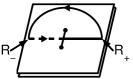
Figure 15. Riemann surface of the function $\arctan$. The solid and dashed lines respectively lie in the upper and the lower leaves. The ramification points correspond to the complex numbers i and -i.

Using Eqs. (105) and (106), one sees that the limits of $\Theta$ when $h\to 0^{\pm}$ correspond respectively to the points $R_{+}$ and $R_{-}$ of the Riemann surface (see Fig. 15). Since these two limit points are the initial and final points of $\Gamma_{R}$, we can associate to $\Gamma_{R}$ the real path from $R_{-}$ to $R_{+}$ of the Riemann surface of the function $\arctan$. The complex continuation of the function $\Theta$ along the small semi-circle $\Gamma_{C}$ of the bifurcation diagram is associated to the big circle at infinity of Fig. 15. From Fig. 15, we thus recover that after a real loop $\Gamma$ locally deformed to the complex domain to bypass the line $C$ the function $\Theta$ has a jump of $\frac{2\pi}{n}$. This result is also coherent with the analysis performed with the variation of the cycles $\delta$. We denote by $\delta_{k}$ the cycle between the ramification points $x_{k}$ and $x_{k+1}$. The cycle is oriented from $x_{k}$ to $x_{k+1}$ in the upper leaf and from $x_{k+1}$ to $x_{k}$ in the lower one. Following the proof of proposition 5, it can be shown that if we compute $\Theta$ along one of these cycles then we obtain asymptotically the same result. More precisely, we have

(215) $$\frac{h}{2}\int_{\delta_{k}(h,j)}\frac{dx}{xy}=\frac{2\pi}{n}\ ,$$

for $j<0$ fixed and $h\to 0^{-}$. We consider now $r$ semi-circles around $C$. The cycle $\delta$ is transformed into $\delta+\delta_{0}-\delta_{1}+\delta_{2}-\cdots+(-1)^{r-1}\delta_{r-1}$. This is displayed for $r=3$ in Figs. 14. As expected, we thus see that after an even (resp. odd) number of semi-circles, the function $\Theta$ has no jump (resp. a jump of $\frac{2\pi}{n}$) which corresponds to the behavior of the complex $\arctan$.

3.5. Generalization to $m:-n$ resonance

We now study the $m:-n$ resonant system with $m>1$ and $m$ and $n$ relatively prime. We associate to such a system a Riemann surface which can be constructed in the variables $x=\pi_{1}+j$ or $x^{\prime}=\pi_{1}-j$ from

(216) $$y^{2}=x^{n}(x-2j)^{m}-[h-R(x-j,j)]^{2}\ ,$$

or

(217) $$y^{2}=(x^{\prime}+2j)^{n}x^{\prime m}-[h-R(x^{\prime}+j,j)]^{2}\ .$$

One passes from one representation to the other by the relation $x=x^{\prime}-2j$. In particular, the two surfaces have the same ramification points translated by $2j$. Depending on the line of singularities considered, one or the other surface will be used, i.e., the surface in $x$ for $j<0$ and the surface in $x^{\prime}$ for $j>0$. We next recall that the discriminant locus $\Delta$ of such a system is given by Eqs. (136). From the expansion of the roots of the polynomial $Q$ in $h=0$ (lemma 7), we deduce that for $j<0$ (resp. $j>0$), $n$ (resp. $m$) roots in $x$ (resp. in $x^{\prime}$) exchange their positions along a loop around the line $C$. We locally deform $\Gamma$ in a neighborhood of the line $C$ and we decompose this loop into four loops $\Gamma_{R_{1}}$, $\Gamma_{R_{2}}$, $\Gamma_{C_{1}}$ and $\Gamma_{C_{2}}$ where $\Gamma_{C_{1}}$ and $\Gamma_{C_{2}}$ are respectively two semi-circles around the lines of singularities $(h=0,j<0)$ and $(h=0,j>0)$. $\Gamma_{R_{1}}$ and $\Gamma_{R_{2}}$ complete the loop $\Gamma$ respectively for $h<0$ and $h>0$. We define the variations of the functions $\Theta$ and $\tau$ along $\Gamma$ as follows

(220) $$\left\{\begin{array}[]{ll}\Delta\Theta_{\Gamma}=\Delta\Theta_{\Gamma_{C_{1}}}+\Delta\Theta_{\Gamma_{C_{2}}}+\Delta\Theta_{\Gamma_{R_{1}}}+\Delta\Theta_{\Gamma_{R_{2}}}\\ \Delta\tau_{\Gamma}=\Delta\tau_{\Gamma_{C_{1}}}+\Delta\tau_{\Gamma_{C_{2}}}+\Delta\tau_{\Gamma_{R_{1}}}+\Delta\tau_{\Gamma_{R_{2}}}\\ \end{array}\right.\ ,$$

where the different variations are determined asymptotically, i.e., when the radii of the semi-circles $C_{1}$ and $C_{2}$ go to 0. A simple calculation then show that the study of the $m:-n$ resonance can be reduced to the study of two cases for $j>0$ and $j<0$ similar to the $1:-n$ resonance. This allows to compute the jump of the function $\Theta$ along $\Gamma$ and to deduce the monodromy matrix for the real loop $\Gamma$. We recover the result of proposition 3.

4. Conclusion

In this paper, we have investigated the notion of Fractional Hamiltonian Monodromy in the 1:-2, $1:-n$ and $m:-n$ resonant systems. We have discussed our asymptotic method to calculate the monodromy matrix in the real approach and we have proposed a definition of fractional monodromy using a complex extension of the bifurcation diagram. From this definition, we have recovered the results of the real approach. At this point, the question which naturally arises is the generalization of this concept to other types of singularities. A part of the answer could be given by applying the complex approach to a new generalization of standard monodromy, the bidromy which has been recently introduced in Ref. [SZ07].

Appendix A Geometric construction

A.1. 1:-2 resonance

As stated in the introduction, the geometric construction of fractional monodromy generalizes the construction of standard monodromy. We propose a schematic representation that is slightly different from the original one proposed in Ref. [NSZ06]. This representation has the advantage to be easily generalizable to 1:-n resonant systems. We use a standard representation of a torus i.e. a rectangle whose edges are identified according to the arrows. The crossing of the line $C$ is displayed in Figs. 16 and 17. A curled torus is represented by two rectangles glued along a horizontal edge and with a particular identification of the vertical edges (see Figs. 16, $h=0$). This construction is not limited to a given energy-momentum map but can be applied to any energy-momentum map having a bifurcation diagram with such a line of singularities.

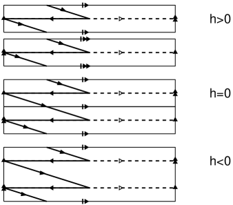
Figure 16. Schematic representation of the continuous transport of the basic cycles $(\beta_{1},\beta_{2})$ when the singular line $C$ is crossed. $\gamma_{1}$ and $\gamma_{2}$ are respectively represented in dashed and solid lines.

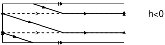
Figure 17. Schematic representation of the basis cycles for $h<0$. Representatives of $[\beta_{1}]$ and $[2\beta_{2}]$ are respectively represented in dashed and solid lines.

Let $\beta_{1}$ and $\beta_{2}$ be the two cycles associated to the flows of $X_{1}$ and $X_{2}$ defined in Eqs. (16). They are the representatives of the classes of homology $[\beta_{1}]$ and $[\beta_{2}]$ which form a basis of $H_{1}(T^{2}(h,j),\mathbb{Z})$ where $(h,j)\in\mathcal{R}_{reg}$. Only a subgroup of $H_{1}$ can be transported continuously across the line $C$. We assume that a basis for this subgroup is given by $[\beta_{1}]$ and $[2\beta_{2}]$. $2\beta_{2}$ corresponds to the cycle $\beta_{2}$ covered twice. For $h>0$, as representatives of $[\beta_{1}]$ and $[2\beta_{2}]$ we consider the two cycles $\gamma_{1}=\beta_{1}$ and $\gamma_{2}$. The cycle $\gamma_{2}$ is the union of two cycles $\beta_{2}$ with starting points belonging to the same orbit of the flow of $X_{1}$ but separate by an angle $\theta=\pi$. To make a link with analytical calculations, $\Theta$ is taken to be $\pi/2$ in this case. $\gamma_{1}$ can be easily transported across $C$ and it remains unchanged. To transport continuously $\gamma_{2}$, the two cycles forming $\gamma_{2}$ have to be connected in one point in $h=0$ and then merged to form only one cycle covered once for $h<0$. Representatives of the basis of $H_{1}(F^{-1}(h,j),\mathbb{Z})$ for $h<0$ are given in Fig. 17, note that $\Theta=-\pi/2$ since $\Theta$ has a discontinuity of size $\pi$ on $C$. Comparison of Fig. 16 ($h<0$) and Fig. 17 leads to the conclusion that after one loop, the cycle $\gamma_{2}$ becomes a representative of the equivalence class $[2\beta_{2}-\beta_{1}]$ and that the corresponding monodromy matrix written formally in the basis $([\beta_{1}],[\beta_{2}])$ is given by

(223) $$M=\left(\begin{array}[]{cc}1&0\\ -1/2&1\end{array}\right)\ .$$

A.2. 1:-n resonance

The geometric construction of Sec. A.1 can be straightforwardly generalized to other resonances. We consider the resonance 1:-3 but other resonances can be treated along the same lines. The 3-curled torus is represented in Fig. 18 ($h=0$) by three rectangles glued along a common edge. Note also the particular identification of the vertical edges. Following notations of Sec. A.1, a basis of the subgroup of $H_{1}(F^{-1}(h,j),\mathbb{Z})$ which can be transported continuously across $C$ is given by $[\beta_{1}]$ and $[3\beta_{2}]$. For $h>0$, as a representative of $[3\beta_{2}]$ we choose three cycles $\beta_{2}$ whose starting points belong to the same orbit of the flow of $X_{j}$ with an angle $\theta$ of $2\pi/3$ between each other. We also assume that $\Theta=\pi/3$ in this case. After crossing $C$, this cycle belongs for $h<0$ to the equivalence class $[3\beta_{2}-\beta_{1}]$ as shown by Fig. 19. For $h<0$, $\Theta=-\pi/3$ since the discontinuity of $\Theta$ on $C$ is equal to $2\pi/3$. In the basis $([\beta_{1}],[\beta_{2}])$, the monodromy matrix $M$ is given by

(226) $$M=\left(\begin{array}[]{cc}1&0\\ -1/3&1\end{array}\right)\ .$$

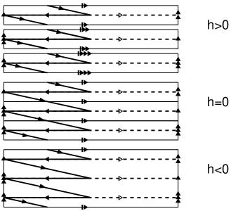
Figure 18. Same as Fig. 16 but for the 1:-3 resonance.

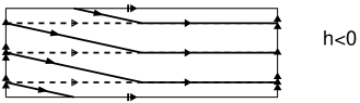
Figure 19. Same as Fig. 17 but for the 1:-3 resonance.

Appendix B The semi-classical point of view

We illustrate in this section the relation between classical monodromy and its semi-classical counterpart for $1:-n$ and $m:-n$ resonant systems. To our knowledge, this point has not been discussed up to now in the literature. We refer the reader to Refs. [Ngoc99, NSZ06] for a rigorous definition of this semi-classical point of view. Here, we consider only the graphical representations of semi-classical monodromy as a pictorial illustration of classical monodromy.

We consider two quantum differential operators $\hat{J}$ and $\hat{H}$ whose classical limits are the Hamiltonians $J$ and $H$. These two operators commute i.e. $[\hat{J},\hat{H}]=0$. They thus have a system of common eigenfunctions belonging to $L^{2}(\mathbb{R}^{2},dq_{1}\wedge dq_{2})$. The corresponding eigenvalues form the quantum joint spectrum of the energy-momentum map $F$ which is a 2-dimensional lattice of points. We can construct the quantum-classical bifurcation diagram of $F$ by superimposing both the quantum joint spectrum and the classical bifurcation diagram. This has been done for the $1:-n$ and $m:-n$ resonant systems in Figs. 20 and 21. Note that the quantum joint spectrum is defined for a given value $\hbar$ viewed here as a parameter. Using EBK quantification rules, we also introduce the semi-classical joint spectrum which is defined as the set of points $(h,j)\in\mathcal{R}_{reg}$ where the numbers $n_{1}$ and $n_{2}$ given by the relations

(227) $$\hbar(n_{i}+\frac{\alpha_{i}}{4})=\oint_{\gamma_{i}}\textbf{pdq}\ ,$$

are integers. In Eq. (227), pdq is the Liouville 1-form and $\alpha_{i}$ the Maslov index associated to the cycle $\gamma_{i}$ where $([\gamma_{1}],[\gamma_{2}])$ is a basis of $H_{1}(T^{2}(h,j),\mathbb{Z})$. We remark that the semi-classical lattice differs from the quantum lattice by $o(\hbar)$ which is irrelevant in our study. We also point out that the EBK quantification rules are not valid near the line of singularities $C$ and have to be replaced by singular rules[dVN03]. In contrast, the quantum joint spectrum gives a smooth transition of the crossing $C$. Moreover, locally around a regular value of $\mathcal{R}$, this lattice is regular in the sense that there exists a map which sends this lattice to $\hbar\mathbb{Z}^{2}$ as $\hbar$ tends to zero. A systematic approach has been developed to check the regularity of the global spectrum. The method consists in taking a cell i.e. a quadrilateral whose vertices lie on the points of the lattice, transporting continuously this cell along a loop $\Gamma$ and comparing the final cell with the initial one. If the two cells are different then the system has quantum monodromy. The rotation matrix which sends the initial cell to the final one is the quantum monodromy matrix $M_{Q}$. More precisely, if the cell is supported by the two vectors $(w_{1},w_{2})$ and if after a loop these vectors are transformed into $(w_{1}^{\prime},w_{2}^{\prime})$ then $M_{Q}$ is defined by the relation

(232) $$\left(\begin{array}[]{c}w^{\prime}_{1}\\ w^{\prime}_{2}\end{array}\right)=M_{Q}\left(\begin{array}[]{c}w_{1}\\ w_{2}\end{array}\right)\ .$$

Using the semi-classical joint spectrum, it can be shown that $M_{Q}=(M_{Cl}^{t})^{-1}$ where $M_{Cl}$ is the classical monodromy matrix. We recall that when the system has fractional monodromy the size of the cell has to be increased to cross the line of singularities. In a way analogous to the classical case, a simple cell cannot be transported continuously across the line $C$. The multiple cell then becomes the basic cell which is equivalent to consider only a sublattice of the original lattice. Here, the vertical lines of the quantum bifurcation diagram which are parallel to $w_{1}$ are labeled by $n_{1}$, the quantum number associated to $\varphi_{J}$ which is a global quantum number. The cells are thus multiplied in the other direction. For instance, for the resonance 1:-3 the size is multiplied by 3. This point is displayed in Fig. 20. For a resonance $m:-n$, due to the form of the monodromy matrix the size is increased from 1 to $mn$ which explains why we have considered cells of size 6 in Fig. 21 for the 2:-3 resonance. Examination of Figs. 20 and 21 shows that in the basis $(w_{1},w_{2})$ the quantum monodromy matrices are respectively equal to

(235) $$\left(\begin{array}[]{cc}1&1/3\\ 0&1\end{array}\right)\ ,$$

for the 1:-3 resonance and

(238) $$\left(\begin{array}[]{cc}1&1/6\\ 0&1\end{array}\right)\ ,$$

for the 2:-3 resonance.

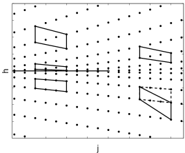
Figure 20. Semi-classical bifurcation diagram for the resonance $1:-3$ and the energy-momentum map of Eqs. (75). The line of singularities $C$ is represented by a solid line. The open dot indicates the position of the origin of the bifurcation diagram. The final cell after a counterclockwise closed loop around the origin is depicted in dashed lines.

Figure 21. Same as Fig. 20 but for the 2:-3 resonance. The corresponding energy-momentum map is given by Eqs. (241).

The energy-momentum map used for the 2:-3 resonance is defined by

(241) $$F=\left\{\begin{array}[]{ll}J\\ \pi_{3}+(\pi_{1}+J)(\pi_{1}-J)\\ \end{array}\right.\ .$$

Appendix C Reduction in the complex approach

We detail in this section the reduction in the complex approach for an $m:-n$ resonant system. This reduction is different from the reduction used in the real approach which is associated to the $S^{1}$-action of the flow of the Hamiltonian $J$. Both reductions leave invariant the polynomials $(J,\pi_{1},\pi_{2},\pi_{3})$ defined by Eqs. (68).

We start from the complexified phase space $T^{*}\mathbb{C}^{2}$ with $(p_{1},q_{1},p_{2},q_{2})\in\mathbb{C}^{4}$. The reduction is based on two $SO(2,\mathbb{C})$ actions $\Phi_{1}$ and $\Phi_{2}$. We recall that a matrix $R\in SO(2,\mathbb{C})$ is a $2\times 2$ matrix which reads

(244) $$\left(\begin{array}[]{cc}a&-b\\ b&a\end{array}\right)\ ,$$

where $(a,b)\in\mathbb{C}^{2}$ and $a^{2}+b^{2}=1$. $\Phi_{k}$ ($k\in\{1,2\}$) is a map from $SO(2,\mathbb{C})\times\mathbb{C}^{2}$ to $\mathbb{C}^{2}$ which associates to each couple $\big{(}R,(q_{k},p_{k})\big{)}$ the point of coordinates

(251) $$\left(\begin{array}[]{cc}a_{k}&-b_{k}\\ b_{k}&a_{k}\end{array}\right)\left(\begin{array}[]{c}q_{k}\\ p_{k}\end{array}\right)=\left(\begin{array}[]{cc}a_{k}q_{k}-b_{k}p_{k}\\ b_{k}q_{k}+a_{k}p_{k}\end{array}\right)\ .$$

We next introduce new coordinates which can be written as follows

(256) $$\left\{\begin{array}[]{llll}\eta_{1}=q_{1}-ip_{1}\\ \xi_{1}=q_{1}+ip_{1}\\ \eta_{2}=q_{2}-ip_{2}\\ \xi_{2}=q_{2}+ip_{2}\\ \end{array}\right.\ .$$

Under the action of $\Phi_{k}$, these new coordinates transform into $\lambda_{k}\xi_{k}$ and $\lambda_{k}^{-1}\eta_{k}$ where $\lambda_{k}=a_{k}+ib_{k}$. Finally, simple algebra shows that the complexified invariant polynomials $(J,\pi_{1},\pi_{2},\pi_{3})$ are invariant under the conjoint action of $\Phi_{1}$ and $\Phi_{2}$ if $\lambda_{1}^{n}\lambda_{2}^{m}=1$. One can conclude that the reduction is associated to a $\mathbb{C}^{*}$-action $\Phi$ from $\mathbb{C}^{*}\times\mathbb{C}^{4}$ to $\mathbb{C}^{4}$ defined as follows

(257) $$\Phi:\big{(}\lambda,(\xi_{1},\eta_{1},\xi_{2},\eta_{2})\big{)}\to(\lambda^{m}\xi_{1},\lambda^{-m}\eta_{1},\lambda^{-n}\xi_{2},\lambda^{n}\eta_{2})\ .$$

References

- [Dui80] J. J. Duistermaat, Commun. Pure Appl. Math. 33, 687 (1980).
- [CB97] R. H. Cushman and L. Bates, Global Aspects of Classical Integrable Systems (Birkhauser, Basel, 1997).
- [Ngoc99] S. V. Ngoc, Comm. Math. Phys. 203, 465 (1999).
- [AKE04] C. A. Arango, W. W. Kennerly, and G. S. Ezra, Chem. Phys. Lett. 392, 486 (2004).
- [SC00] D. A. Sadovskií and R. H. Cushman, Physica D 142, 166 (2000).
- [KR03] I. N. Kozin and R. M. Roberts, J. Chem. Phys. 118, 10523 (2003).
- [CWT99] M. S. Child, T. Weston, and J. Tennyson, Mol. Phys. 96, 371 (1999).
- [SZ99] D. A. Sadovskií and B. I. Zhilinskií, Phys. Lett. A 256, 235 (1999).
- [WJD03] H. Waalkens, A. Junge, and H. R. Dullin, J. Phys. A 36, L307 (2003).
- [GCSZ04] A. Giacobbe, R. H. Cushman, D. A. Sadovskií, and B. I. Zhilinskií, J. Math. Phys. 45, 5076 (2004).
- [EJS04] K. Efstathiou, M. Joyeux, and D. A. Sadovskií, Phys. Rev. A 69, 032504 (2004).
- [NSZ02] N. N. Nekhoroshev, D. A. Sadovskií, and B. I. Zhilinskií, C. R. Acad. Sci. Paris 335, 985 (2002).
- [NSZ06] N. N. Nekhoroshev, D. A. Sadovskií, and B. I. Zhilinskií, Ann. Inst. H. Poincaré Phys. Theor. 7, 1099 (2006).
- [Efs04] K. Efstathiou, Metamorphoses of Hamiltonian Systems with Symmetry (Springer-Verlag, Heidelberg, 2004).
- [ECS07] K. Efstathiou, R. H. Cushman, and D. A. Sadovskií, Adv. in Math. 209, 241 (2007).
- [Nek07] N. N. Nekhoroshev, Sbornik : Mathematics 198, 383 (2007).
- [Arn89] V. I. Arnol’d, Mathematical Methods of Classical Mechanics (Springer-Verlag, New York, 1989).
- [Aud02] M. Audin, Comm. Math. Phys. 229, 459 (2002).
- [Viv03] O. Vivolo, J. Geom. Phys. 46, 99 (2003).
- [BC01] F. Beukers and R. H. Cushman, University of Utrecht (2001).
- [dVP99] Y. C. de Verdière and B. Parisse, Comm. Math. Phys. 205, 459 (1999).
- [Ngoc00] S. V. Ngoc, Comm. Pure Appl. Math. 53, 143 (2000).
- [dVN03] Y. C. de Verdière and S. V. Ngoc, Ann. Ec. Norm. Sup. 36, 1 (2003).
- [Vor83] A. Voros, Ann. Inst. H. Poincaré Phys. Theor. 39, 211 (1983).
- [DDP97] E. Delabaere, H. Dillinger, and F. Pham, J. Math. Phys. 38, 6126 (1997).
- [DP97] E. Delabaere and F. Pham, Ann. of Phys. 261, 180 (1997).
- [AGZV88] V. I. Arnol’d, Goussein-Zade, and Varchenko, Singularities of differentiable mappings (Birkhauser, Boston, 1988).
- [Zol06] H. Zoladek, The Monodromy group (Birkhauser, Boston, 2006).
- [Bat91] L. M. Bates, J. Appl. Math. Phys. 42, 837 (1991).
- [Kir93] F. Kirwan, Complex Algebraic Curves (Cambridge University Press, Cambridge, 1993).
- [Wolf64] J. A. Wolf, Mich. Math. J. 11, 65 (1964).
- [SZ07] D. A. Sadovskií and B. I. Zhilinski’i, Ann. of Phys. 322, 164 (2007).