Approximate Model of Neutron Resonant Scattering in a Crystal

Abstract

In the theory of resonant scattering, the double differential cross section involves the computation of a multifold integral of a 4-point correlation function, which generalizes the traditional 2-point correlation function of Van-Hove for potential scattering. In the case of a neutron-crystal interaction, the numerical computation of these multifold integrals is cumbersome. In this paper, a new approximation is suggested. It is based on a factorization of the differential cross section into one function describing the exchange of kinetic energy between the neutron and the bound nucleus (phonons dynamic) and a function related to the nuclear scattering amplitude. This formalism is then applied to the modeling of resonant scattering of a neutron by ${}^{238}U$ in a $UO_{2}$ crystal lattice.

1 Introduction

The computation of the double differential scattering cross section (DDCS) at low incident neutron energies is required to solve neutron transport problems. Wigner and Wilkins [1] used a two-body kinematic approach to study potential scattering in a free gas. Under the same classic assumptions, Blackshaw and Murray [2] studied the case of an energy-dependent cross section and further generalizations were investigated by Ouisloumen and Sanchez [3] and Rothenstein and Dagan [4].

A general quantum formalism due primarily to Van Hove [5] expresses the DDCS of potential scattering by a bound nucleus as a Fourier transform of a 2-point correlation function. Kazarnovski et al. [8] and Word and Trammell [7] extended the Van Hove theory to study resonant processes. The resonant DDCS becomes a Fourier double-Laplace transform of a 4-point correlation function.

In the case of a harmonic crystal, the numerical computation of the multifold integral is difficult because of the highly oscillating behavior of the 4-point correlation function. A simplified multiphonon model, known as the ”uncoupled phonon approximation” (UPA) was proposed by Naberejnev [9]. However, the validity of this approximation is questioned especially within the short time range (case of high temperature for instance). The present work suggests a new approximation that gives a correct limit at short time and provides a simple formula to compute the scattering kernel.

2 General formalism

2.1 The 4-point correlation function

When the scattering amplitude is independent of incident neutron energy, it is known since the work of Van Hove [5] that the scattering DDCS is related to the Fourier transform of a two point correlation function $\chi_{2}(\tau)$ :

$$\frac{d^{2}\sigma}{d\Omega dE_{f}}=\frac{\sigma_{p}}{4\pi}\frac{k_{f}}{k_{i}}\mathcal{F}\{\chi_{2}(\tau)\}(\Delta E).$$ (1)

$\Delta E=E_{f}-E_{i}$ is the energy transfer with $E_{i}$ and $E_{f}$ the energy of the neutron before and after the scattering event. The Fourier transform is defined as

$$\mathcal{F}\{\chi_{2}(\tau)\}(x)=\frac{1}{2\pi}\int_{-\infty}^{\infty}e^{-ix\tau}\chi_{2}(\tau)d\tau.$$ (2)

$\mathcal{F}\{\chi_{2}(\tau)\}(\Delta E)$ is the usual scattering function $S(\alpha,\beta)=S(\vec{\Delta k},\Delta E)$ which depends on the momentum transfer $\vec{\Delta}k=\vec{k}_{f}-\vec{k}_{i}$ where $\vec{k}_{i}$ and $\vec{k}_{f}$ are the initial and final neutron wave vector respectively . The theory was later generalized to treat the case of resonant scattering [7]. In the incoherent approximation, the scattering cross section includes the resonant, the potential-resonant interference and potential terms. It can be demonstrated that the DDCS of the resonant term for instance is related to the Fourier-double-Laplace transform $\mathcal{L}_{2}\mathcal{F}$ of a 4-point correlation function $\chi_{4}(\tau,t,t^{\prime})$:

$$\frac{d^{2}\sigma}{d\Omega dE_{f}}=\frac{\sigma_{m}}{4\pi}\frac{\Gamma_{n}}{\Gamma}\frac{k_{f}}{k_{i}}\frac{\Gamma^{2}}{4}\mathcal{L}_{2}\mathcal{F}\{\chi_{4}(\tau,t,t^{\prime})\}(\Delta E,-i(E_{i}-E_{0})+\Gamma/2,+i(E_{i}-E_{0})+\Gamma/2).$$ (3)

$E_{0}$, $\Gamma_{n}$ and $\Gamma$ are the energy, the neutron and total width of the resonance. $\sigma_{m}=4\pi g\Gamma_{n}/k_{i}^{2}\Gamma$ and $g$ is the usual statistical spin factor. The Fourier-double-Laplace transform is defined as

$$\mathcal{L}_{2}\mathcal{F}\{f(\tau,t,t^{\prime})\}(x,z1,z2)=\frac{1}{2\pi}\int_{-\infty}^{\infty}\int_{0}^{\infty}\int_{0}^{\infty}e^{-ix\tau}e^{-z_{1}t}e^{-z_{2}t^{\prime}}\ f(\tau,t,t^{\prime})d\tau dtdt^{\prime}.$$ (4)

Similarly, the resonant-potential interference term is expressed as a Fourier-single-Laplace transform of a 3 point correlation function $\chi_{3}(\tau,t)$.

A quantum calculation shows that $\chi_{4}(\tau,t,t^{\prime})$ is a function of time-dependant displacement operators:

$$\chi_{4}(\tau,t,t^{\prime}) = <\exp\left(-i\vec{k}_{i}.\vec{r}(\tau+t-t^{\prime})\right)\exp\left(i\vec{k}_{f}.\vec{r}(\tau+t)\right)$$ (5)

$$\times \exp\left(-i\vec{k}_{f}.\vec{r}(t)\right)\exp\left(i\vec{k}_{i}.\vec{r}(0)\right)>_{T}.$$

Note that $\chi_{2}(\tau)=\chi_{4}(\tau,0,0)$ and $\chi_{3}(\tau,t)=\chi_{4}(\tau,t,0)$. $<X>_{T}$ denotes the thermal average at temperature $T$. In this paper, time $\tau$, $t$ and $t^{\prime}$ are expressed in unit of energy and $\hbar=1$. The right hand side of Equation 1 and 3 should be multiplied by $\left(\frac{M+m}{m}\right)^{2}$ which is implicitly assumed in the paper. $M$ and $m$ are the mass of the target nucleus and incident neutron and $A=M/m$ respectively . The scattering is assumed isotropic in the center-of-mass frame and multiple scattering effects are neglected (single collision approximation). Equation 3 assumes that the Hamiltonian of the target and compound nucleus is the same. This condition neglects the mass change of the target nucleus when the neutron is absorbed and re-emitted: $M>>m$.

2.2 Free-gas versus harmonic crystal-lattice model

In the case where the target nucleus behaves like a free gas, the displacement operator is proportional to the momentum operator $r(t)=r(0)+p(0)t/M$. After averaging over a Maxwellian distribution of momentum at temperature $T$, $\chi_{4}$ within the free gas model (FGM) becomes

$$\chi_{4}(\tau,t,t^{\prime})=\exp\{\frac{-i}{2M}[\tau(\vec{k}_{f}-\vec{k}_{i})^{2}+(t-t^{\prime})k_{i}^{2}]-\frac{kT}{2M}[-\vec{k}_{i}(t-t^{\prime})+\tau(\vec{k}_{f}-\vec{k}_{i})]^{2}\}.$$ (6)

When the target nucleus is bound to a crystal lattice, the 4-point correlation function is more complex. Under the harmonic approximation, the Bloch theorem [9] transforms $\chi_{4}$ into

$$\chi_{4}(\tau,t,t^{\prime})=\exp\{-\rho(\vec{k}_{i},\vec{k}_{i},0)-\rho(\vec{k}_{f},\vec{k}_{f},0)\}$$

$$\times\exp\{\rho(\vec{k}_{i},\vec{k}_{f},-t^{\prime})+\rho(\vec{k}_{f},\vec{k}_{i},+t)+\rho(\vec{k}_{f},\vec{k}_{f},\tau)\}$$

$$\times\exp\{\rho(\vec{k}_{i},\vec{k}_{i},\tau-t^{\prime}+t)-\rho(\vec{k}_{i},\vec{k}_{f},\tau-t^{\prime})-\rho(\vec{k}_{f},\vec{k}_{i},\tau+t)\}.$$ (7)

For a cubic lattice with a phonon density of states $\rho(\omega)$,

$$\rho(\vec{k},\vec{k}^{\prime},+t)=\frac{\vec{k}.\vec{k}^{\prime}}{2M}{\int_{0}^{\infty}d\omega\frac{\rho(\omega)}{\omega}[coth(\omega/2kT)cos(\omega t)-isin(\omega t)]}.$$ (8)

In the short time approximation for $\tau$, $t$, and $t^{\prime}$ the DDCS can be simplified using

$$\rho(k,k^{\prime},+t)\approx\rho(k,k^{\prime},0)+\vec{k}.\vec{k}^{\prime}(\frac{-kT_{eff}}{2M}t^{2}-\frac{it}{2M}),$$ (9)

with

$$kT_{eff}=\frac{1}{2}\int_{0}^{\infty}d\omega\rho(\omega)\omega coth(\omega/2kT).$$ (10)

Plugging 9 into 2.2, we get the free gas formula 6 with $T_{eff}$ instead of $T$. Consequently, the crystal-lattice model lead to the free gas model, with an effective temperature, when $\tau$, $t$, and $t^{\prime}$ are small (short time approximation). This is the same effective temperature as Lamb [12] derived for the Doppler broadening of a capture resonance in a solid in the weak binding limit.

2.3 The uncoupled phonon approximation

The UPA approximation proposed in [9] was an attempt to compute the resonant scattering kernel for a harmonic crystal. It neglected $t$ and $t^{\prime}$ in the coupling terms $\rho(\vec{k}_{i},\vec{k}_{i},\tau-t^{\prime}+t)$, $\rho(\vec{k}_{i},\vec{k}_{f},\tau-t^{\prime})$ and $\rho(\vec{k}_{f},\vec{k}_{i},\tau+t)$ in Equation 2.2 and applied a short time approximation to $\rho(\vec{k}_{i},\vec{k}_{f},-t^{\prime})$ and $\rho(\vec{k}_{f},\vec{k}_{i},+t)$ . The correlation function becomes

$$\chi^{UPA}_{4}(\tau,t,t^{\prime}) = \exp\left(\rho(\vec{\Delta k},\tau)-\rho(\vec{\Delta k},0)\right)$$ (11)

$$\times \exp\left(\vec{k_{i}}\vec{k_{f}}[\frac{-kT_{eff}}{2M}(t^{2}+t^{\prime 2})-\frac{i(t-t^{\prime})}{2M}]\right).$$

The integral over $\tau$ and $t,t^{\prime}$ can be performed separately. Since the first exponential is the Van-Hove function $\chi_{2}(\tau)$, the differential cross section can be factored out as

$$\frac{d^{2}\sigma}{d\Omega dE}=\frac{1}{4\pi}\frac{k_{f}}{k_{i}}\times S(\vec{\Delta k},\Delta E)\times\tilde{\sigma}(\vec{k}_{i},\vec{k}_{f}).$$ (12)

The detailed mathematical expression for the so-called UPA cross section $\tilde{\sigma}(\vec{k}_{i},\vec{k}_{f})$ can be found in [9]. The UPA model separates the phonon dynamic and the nuclear interaction and provides a rather simple way to compute DDCS. However, within the UPA approximation, the 4-point correlation for small $\tau$, $t$, and $t^{\prime}$ becomes

$$\chi^{UPA}_{4}(\tau,t,t^{\prime})=\exp\{\frac{-i}{2M}[\tau(\vec{k}_{f}-\vec{k}_{i})^{2}+(t-t^{\prime})\vec{k}_{i}\vec{k}_{f}]-\frac{kT_{eff}}{2M}[\vec{k}_{i}\vec{k}_{f}(t^{2}+t^{\prime 2})+\tau^{2}(\vec{k}_{f}-\vec{k}_{i})^{2}]\},$$ (13)

which differs markedly from the required equation 6 discussed in the previous section. Consequently, the DDCS within the UPA approximation does not give the correct limit for small $t$ and $t^{\prime}$.

3 Proposed Model

Our model seeks to get a factorization of the DDCS similar to the UPA model:

$$\frac{d^{2}\sigma}{d\Omega dE}=\frac{1}{4\pi}\frac{k_{f}}{k_{i}}\times S(\vec{\Delta k},\Delta E)\times\tilde{\sigma}(\vec{k}_{i},\vec{k}_{f}).$$ (14)

However, in order to get the correct limit at short time, we computed the $\tilde{\sigma}$ term using the short time approximation of the correlation function (Equation 6), without the previous UPA approximation.

For values of $\vec{\Delta k}\neq\vec{0}$, the following notation is used,

$$\Delta=\sqrt{\frac{4kT}{M}\frac{k_{i}^{2}k_{f}^{2}-(\vec{k}_{i}\vec{k}_{f})^{2}}{2\vec{\Delta k}^{2}}}\ \ x=2\ [E_{i}-E_{0}-(E_{f}-E_{i})\ \frac{\vec{k}_{i}\vec{\Delta}k}{\vec{\Delta k}^{2}}-\frac{\vec{k}_{i}\vec{k}_{f}}{2M}]\ /\ \Gamma.$$ (15)

It is found that the differential cross section, including resonant, potential and resonant-potential interference can be calculated almost analytically and can be split into nuclear and transfer terms. The details of the demonstration are presented in the Appendix. The final result is:

$$\frac{d^{2}\sigma}{d\Omega dE}=\frac{1}{4\pi}\frac{k_{f}}{k_{i}}\times S(\vec{\Delta k},\Delta E)\times[\ \sigma_{p}+\sigma_{m}\frac{\Gamma_{n}}{\Gamma}\psi+\sqrt{\sigma_{p}\sigma_{m}\frac{\Gamma_{n}}{\Gamma}}\chi\ ].$$ (16)

For $\Delta\neq 0$ and $\vec{\Delta k}\neq\vec{0}$,

$$\psi=\frac{\sqrt{\pi}}{2}\times\frac{\Gamma}{\Delta}K(\frac{x\Gamma}{2\Delta},\frac{\Gamma}{2\Delta})\ \ \ \chi=\sqrt{\pi}\times\frac{\Gamma}{\Delta}L(\frac{x\Gamma}{2\Delta},\frac{\Gamma}{2\Delta}).$$ (17)

For $\Delta=0$ and $\vec{\Delta k}\neq\vec{0}$

$$\psi=\frac{1}{1+x^{2}}\ \ \ \chi=\frac{2x}{1+x^{2}}.$$ (18)

where $K(x,y)$ and $L(x,y)$, are the real and imaginary part of complex complementary error function $w(z)=\exp[-(x+iy)^{2}]\ erfc\ [-i(x+iy)]$, related to the classic Voigt functions.

$$K(x,y)=\Re[w(z)]=\frac{y}{\pi}\int_{-\infty}^{\infty}\frac{\exp(-t^{2})}{(x-t)^{2}+y^{2}}dt$$ (19)

$$L(x,y)=\Im[w(z)]=\frac{x}{\pi}\int_{-\infty}^{\infty}\frac{\exp(-t^{2})}{(x-t)^{2}+y^{2}}dt.$$ (20)

When $\vec{\Delta k}=\vec{0}$, the same calculations lead to Equation 16 with :

$$\Delta=\sqrt{\frac{4kTk_{i}^{2}}{2M}}\ \ x=2\ [E_{i}-E_{0}-\frac{k_{i}^{2}}{2M}]\ /\ \Gamma.$$ (21)

We recognize the usual Doppler-broadened cross section $\sigma^{T}$, so that the differential cross section becomes

$$\frac{d^{2}\sigma}{d\Omega dE}=\frac{1}{4\pi}\frac{k_{f}}{k_{i}}\times S(\vec{\Delta k},\Delta E)\times\sigma^{T^{*}}(E^{*}),$$ (22)

where $T^{*}$ and $E^{*}$ depend on the cosine of the scattering angle $\mu=\cos\theta$:

$$T^{*}(\mu)=T\frac{k_{f}^{2}(1-\mu^{2})}{\vec{\Delta k}^{2}}\ \ \ E^{*}=E_{i}-(E_{f}-E_{i})\ \frac{\vec{k}_{i}\vec{\Delta}k}{\vec{\Delta k}^{2}}-\frac{\vec{k}_{i}\vec{k}_{f}}{2M},$$ (23)

and for $\vec{\Delta k}=\vec{0}$

$$T^{*}=T\ \ \ E^{*}=E_{i}-\frac{\vec{k}_{i}^{2}}{2M}.$$ (24)

Equation 23 is valid only when $E_{i}-(E_{f}-E_{i})\ \frac{\vec{k}_{i}\vec{\Delta}k}{\vec{\Delta k}^{2}}-\frac{\vec{k}_{i}\vec{k}_{f}}{2M}$ is positive. The previous equation can be further simplified noting that $T^{*}\approx T[(1+\mu)/2][1+\Delta E/(2E_{i})]\approx T(1+\mu)/2$ and when $1-\mu>>|\vec{\Delta k}|/|\vec{k}_{i}|$ we have $\frac{\vec{k}_{i}\vec{\Delta}k}{\vec{\Delta k}^{2}}\approx-1/2$ and this approximation produces satisfactory results when used over the whole range of values of $\mu$. Making these approximations, we get a simple formula

$$\frac{d^{2}\sigma}{d\Omega dE}=\frac{1}{4\pi}\frac{k_{f}}{k_{i}}\times S(\vec{\Delta k},\Delta E)\times\sigma^{T(1+\mu)/2}\left([E_{i}+E_{f}]/2-E_{i}\mu/A\right).$$ (25)

Equation 25 provides a simple way to compute the differential cross section within the free gas model. It also gives an approximate way to account for solid state effects by using the known scattering function $S(\vec{\Delta k},\Delta E)$ for the harmonic crystal. Note that Equation 25 was demonstrated for a single resonance and it is not known if this formula can be generalized to any form of free scattering amplitude.

4 Application to neutron resonant scattering in UO₂

Low-enriched uranium oxide UO₂ is widely used as nuclear-reactor fuel. With the present model, the scattering kernel of ²³⁸U in UO₂ has been calculated near the first resonance at 6.67 eV by numerical integration of the differential cross section over scattering angles. The weighted phonon spectrum for ²³⁸U in UO₂ has been taken from the measurement of Dolling et al. [10]. The spectrum features two acoustic modes around 14 and 21 meV.

The $S(\vec{\Delta k},\Delta E)$ Van-Hove scattering function has been computed using the usual phonon expansion methods. The ²³⁸U resonance parameters evaluated by Moxon and Sowerby [11] were used.

The present model has been compared with the classic free gas kernel published by Blackshaw and Murray [2] and studied by Ouisloumen and Sanchez [3]. Fig. 1 and 2 show the resulting scattering kernel at 300 K at two incident neutron energies, 6.674 eV (the peak of the first resonance) and 6.520 eV which is the minimum of the cross section due the interference between the resonant and potential amplitudes. Compared to the UPA model (see Figures in Reference [9]), the present crystal model gives results closer to the free gas model. The only distinctive features are the small peaks around the elastic peak, associated with the one-phonon excitation of the acoustic modes. Note that when the $S(\vec{\Delta k},\Delta E)$ of the FGM is used in Equation 16, the numerical computations give the same results as Ouisloumen and Sanchez.

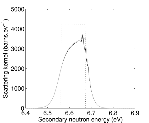
Figure 1: Comparison of scattering kernels calculated with the present formalism (black line) and the free gas model of Ouisloumen and Sanchez [3] (grey line) at incident neutron energy of 6.674 eV. The dotted line is the kernel with a static model.

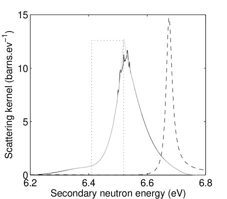
Figure 2: Comparison of scattering kernels calculated with the present formalism (black line) and the free gas model of Ouisloumen and Sanchez [3] (grey line) at incident neutron energy of 6.520 eV. The dotted line is the kernel with a static model and the dashed line is the scattering cross section ($\sigma_{s}/100$ in barns).

5 Conclusion

An approximate formula is proposed to treat solid state effects in neutron-crystal interactions. The DDCS is the product of a Doppler-broadened scattering cross section and the usual Van-Hove scattering function.

$$\frac{d^{2}\sigma}{d\Omega dE}=\frac{1}{4\pi}\frac{k_{f}}{k_{i}}\times S(\vec{\Delta k},\Delta E)\times\sigma^{T(1+\mu)/2}\left([E_{i}+E_{f}]/2-E_{i}\mu/A\right).$$ (26)

This formula gives the correct free-gas limit for short-time range (high-temperature cases). A rigorous calculation of the DDCS within the crystal lattice model is still an open issue. The present work develops the case of a single isolated resonance but further generalizations to multilevel forms of collision matrix may be possible.

In reactor applications, the model predicts small solid-state effects in the scattering of neutrons in UO₂ at 300K, contrary to previous studies using the UPA approximation. Measurements of the secondary spectrum of neutrons scattered elastically in resonances would be valuable to check existing scattering models.

Appendix A Derivation of Equation 16

For $\vec{\Delta k}\neq\vec{0}$, $\chi_{4}$ in Equation 6 can be transformed into

$$\chi_{4} = \exp\{\frac{-i}{2M}[\left(\tau-\frac{\vec{k}_{i}\vec{\Delta}k(t-t^{\prime})}{\vec{\Delta k}^{2}}\right)\vec{\Delta}k^{2}+(t-t^{\prime})\vec{k}_{i}\vec{k}_{f}]$$ (27)

$$- \frac{kT}{2M}[\left(\tau-\frac{\vec{k}_{i}\vec{\Delta}k(t-t^{\prime})}{\vec{\Delta k}^{2}}\right)^{2}\vec{\Delta}k^{2}-\frac{k_{i}^{2}k_{f}^{2}-(\vec{k}_{i}\vec{k}_{f})^{2}}{\vec{\Delta k}^{2}}(t-t^{\prime})^{2}]\}.$$

Using the variable $u=\tau-\vec{k}_{i}\vec{\Delta}k(t-t^{\prime})/\vec{\Delta k}^{2}$, we recognize $\chi_{2}$ the pair correlation function for a free gas:

$$\chi_{2}(u)=\exp\{\frac{-i}{2M}u\vec{\Delta k}^{2}-\frac{kT}{2M}u^{2}\vec{\Delta k}^{2}\}.$$ (28)

Therefore, the Fourier transform of $\chi_{4}$ (integration over $\tau$) will lead to the $S(\vec{\Delta}k,\Delta E)$ terms with a phase factor to account for the change of variable $\tau\rightarrow u$. The DDCS takes the form of Equation 22 with

$$\tilde{\sigma} = \sigma_{m}\frac{\Gamma_{n}}{\Gamma}\frac{\Gamma^{2}}{4}\int_{0}^{\infty}\int_{0}^{\infty}e^{-zt}e^{-z^{*}t^{\prime}}\ \phi(t-t^{\prime})dtdt^{\prime},$$ (29)

with $z=-i\left(E_{i}-E_{0}-\left(E_{f}-E_{i}\right)\frac{\vec{k}_{i}\vec{\Delta}k}{\vec{\Delta k}^{2}}-\frac{\vec{k}_{i}\vec{k}_{f}}{2M}\right)+\frac{\Gamma}{2}$ and

$$\phi(t)=\exp\left(-\frac{kT}{2M}\frac{k_{i}^{2}k_{f}^{2}-(\vec{k}_{i}\vec{k}_{f})^{2}}{\vec{\Delta k}^{2}}t^{2}\right).$$ (30)

To compute the double Laplace transform, the following identity is used:

$$\int_{0}^{\infty}\int_{0}^{\infty}e^{-zt-z^{*}t^{\prime}}\phi(t-t^{\prime})dtdt^{\prime}=\frac{1}{z+z^{*}}\int_{0}^{\infty}e^{-zt}\phi(t)dt+\int_{0}^{\infty}e^{-z^{*}t}\phi^{*}(t)dt.$$ (31)

Equation 29 becomes

$$\tilde{\sigma} = \sigma_{m}\frac{\Gamma_{n}}{4}\int_{0}^{\infty}e^{-i\left(E_{i}-E_{0}-\left(E_{f}-E_{i}\right)\frac{\vec{k}_{i}\vec{\Delta}k}{\vec{\Delta k}^{2}}-\frac{\vec{k}_{i}\vec{k}_{f}}{2M}\right)t+\frac{\Gamma t}{2}}e^{\left(-\frac{kT}{2M}\frac{k_{i}^{2}k_{f}^{2}-(\vec{k}_{i}\vec{k}_{f})^{2}}{\vec{\Delta k}^{2}}t^{2}\right)}dt$$ (32)

$$+ c.c.$$

c.c denotes the conjugate complex. This equation is then reduced into a single integral which can be further simplified using

$$\int_{0}^{\infty}e^{-iat-bt^{2}}dt=\sqrt{\frac{\pi}{b}}\exp\frac{-a^{2}}{4b}erfc\ [\frac{ia}{\sqrt{4b}}]$$ (33)

We recognize in 32 and 33 the real of the complex complementary error function. Equations 16, 17 and 20 are obtained in a similar way when the potential and potential-resonant interference terms are accounted for.

References

References

• [1] Wigner E P and Wilkins E J 1944 AECD-2275, Clinton Laboratory
• [2] Blackshaw G L and Murray R L 1967 Nucl. Sci. Eng. 27, 520–532
• [3] Ouisloumen M and Sanchez R 1991 Nucl. Sci. Eng. 107, 189–200
• [4] Rothenstein W 2004 Ann. Nucl. Energy 31, 1, 9–23
• [5] Van Hove L 1954 Phys. Rev. 95, 249
• [6] Trammel G T 1962 Phys. Rev. 126, 1045
• [7] Word R E and Trammell G T 1981 Phys. Rev. B24, 2430
• [8] Kazarnovskii M V and Stepanov A V 1962 Sov. Phys. JETP, 15, 2, 343–349
• [9] Naberejnev D G 2001 Ann. Nucl. Energy 28, 1
• [10] Dolling G et al. 1965 Can. Journ. Phys. 43
• [11] Moxon M and Sowerby M 1994 Summary of the Work of the NEANDC Task Force on U-238, Nuclear Energy Agency, OECD report
• [12] Lamb W E 1939 Phys. Rev. 55, 190
• [13] Shamaoun A I and Summerfield G C 1990 Ann. Nucl. Energy 17, 229