A Novel Solution to the Frenet-Serret Equations

Abstract

A set of equations is developed to describe a curve in space given the curvature $\kappa$ and the angle of rotation $\theta$ of the osculating plane.  The set of equations has a solution (in terms of $\kappa$ and $\theta$) that indirectly solves the Frenet-Serret equations, with a unique value of $\theta$ for each specified value of $\tau$.  Explicit solutions can be generated for constant $\theta$.  The equations break down when the tangent vector aligns to one of the unit coordinate vectors, requiring a reorientation of the local coordinate system.

1 Introduction

Given the curvature $\kappa$ and torsion $\tau$, the Frenet-Serret equations¹ describe a curve in space parameterized by the arc length $s$:

$$\frac{d\boldsymbol{T}}{ds} =\kappa\boldsymbol{N};$$ (1)

$$\frac{d\boldsymbol{N}}{ds} =-\kappa\boldsymbol{T+}\tau\boldsymbol{B};$$ (2)

$$\frac{d\boldsymbol{B}}{ds} =-\tau\boldsymbol{N};$$ (3)

$$\frac{d\boldsymbol{R}}{ds} =\boldsymbol{T}.$$ (4)

Here $\boldsymbol{R}$, $\boldsymbol{T}$, $\boldsymbol{N}$, and $\boldsymbol{B}$ are the position, tangent, normal, and binormal vectors, respectively.  These equations have no explicit solution (in terms of $\kappa$ and $\tau$) for the general case, although solutions for special cases exist².

It is shown here that a set of equations can be developed to describe a curve in space given the curvature $\kappa$ and the angle of rotation $\theta$ of the osculating plane.  The set of equations has a solution (in terms of $\kappa$ and $\theta$) that indirectly solves the Frenet-Serret equations, and has a unique $\theta$ for every value of $\tau$.

Many problems^3-7 involve the use of the Frenet-Serret equations, requiring numerical approximations or the use of helical arc segments (each having constant $\tau$ and $\kappa$).  Specifying $\kappa$ and $\theta$ to generate a solution may be useful if $\tau$ is not initially known.  The torsion $\tau$ can then be determined from $\theta$.

2 Mathematical Development

A local coordinate system having the property $\boldsymbol{T}=\boldsymbol{i}^{\prime}$ (figure 1) supports the definition of $\boldsymbol{N}$:

$$\boldsymbol{N}=\boldsymbol{j}^{\prime}\cos\theta+\boldsymbol{k}^{\prime}\sin\theta.$$ (5)

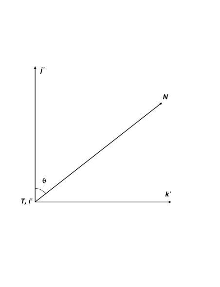
Figure 1: Local coordinate system; $\boldsymbol{T}$ is normal to the plane containing $\boldsymbol{j}^{\prime}$ & $\boldsymbol{k}^{\prime}$.

The curvature $\kappa$ and the angle of rotation $\theta$ of the osculating plane (containing $\boldsymbol{N}$ and $\boldsymbol{T}$) characterize the curve.  When the plane containing $\boldsymbol{T}$ and the global coordinate $\boldsymbol{j}$ is normal to $\boldsymbol{k}^{\prime}$ (figure 2) then

$$\boldsymbol{k}^{\prime}=\frac{\boldsymbol{T}\times\boldsymbol{j}}{\left|\boldsymbol{T}\times\boldsymbol{j}\right|}=\frac{-\boldsymbol{i}T_{k}+\boldsymbol{k}T_{i}}{\sqrt{1-T_{j}^{2}}}.$$ (6)

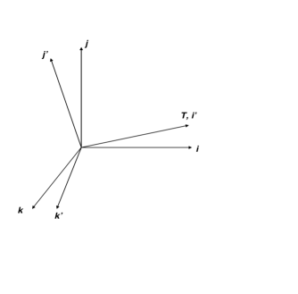
Figure 2: Angular orientation of the local coordinate system with respect to the global coordinate system.

Equation (6) breaks down when $\boldsymbol{T}=\pm\boldsymbol{j}$, requiring an alternate expression for $\boldsymbol{k}^{\prime}$ (developed in section 4).  However, when $\boldsymbol{T}\neq\pm\boldsymbol{j}$,

$$\boldsymbol{j}^{\prime}=\boldsymbol{k}^{\prime}\times\boldsymbol{T}=\frac{-\boldsymbol{i}T_{i}T_{j}+\boldsymbol{j}\left(1-T_{j}^{2}\right)-\boldsymbol{k}T_{j}T_{k}}{\sqrt{1-T_{j}^{2}}}\text{.}$$ (7)

Substituting (7) and (6) into (5):

$$N_{i} =\frac{1}{\kappa}\frac{dT_{i}}{ds}=\frac{-T_{k}\sin\theta-T_{i}T_{j}\cos\theta}{\sqrt{1-T_{j}^{2}}};$$ (8)

$$N_{j} =\frac{1}{\kappa}\frac{dT_{j}}{ds}=\cos\theta\sqrt{1-T_{j}^{2}};$$ (9)

$$N_{k} =\frac{1}{\kappa}\frac{dT_{k}}{ds}=\frac{T_{i}\sin\theta-T_{j}T_{k}\cos\theta}{\sqrt{1-T_{j}^{2}}}.$$ (10)

Equation (9) can be integrated directly:

$$\int_{T_{j0}}^{T_{j}}\frac{dT_{j}}{\sqrt{1-T_{j}^{2}}}=\int_{s_{0}}^{s}\kappa\cos\theta d\sigma;$$ (11)

leading to

$$\sin^{-1}T_{j} =\sin^{-1}T_{j0}+\int_{s_{0}}^{s}\kappa\cos\theta d\sigma;$$

$$T_{j} =\sin\left[\sin^{-1}T_{j0}+\int_{s_{0}}^{s}\kappa\cos\theta d\sigma\right]=\sin\delta;$$

$$T_{j} =T_{j0}\cos\int_{s_{0}}^{s}\kappa\cos\theta d\sigma+\sqrt{1-T_{j0}^{2}}\sin\int_{s_{0}}^{s}\kappa\cos\theta d\sigma.$$ (12)

Equation (8) is solved by noting that $T_{k}=\sqrt{1-T_{j}^{2}-T_{i}^{2}}=\sqrt{\cos^{2}\delta-T_{i}^{2}}$ and introducing the variable $\beta$ so that

$$T_{i} =\cos\delta\cos\beta;$$ (13)

$$T_{k} =\cos\delta\sin\beta.$$ (14)

Substituting into (8):

$$\frac{dT_{i}}{ds} =-\kappa\cos\theta\sin\delta\cos\beta-\cos\delta\sin\beta\frac{d\beta}{ds}$$

$$=\frac{-\kappa\sin\theta\cos\delta\sin\beta-\kappa\cos\theta\cos\delta\cos\beta\sin\delta}{\cos\delta}$$

$$=-\kappa\sin\theta\sin\beta-\kappa\cos\theta\cos\beta\sin\delta.$$ (15)

Equation (15) simplifies to

$$\frac{d\beta}{ds}=\frac{\kappa\sin\theta}{\cos\delta};$$ (16)

or

$$\beta=\beta_{0}+\int_{s_{0}}^{s}\frac{\kappa\sin\theta}{\cos\delta}d\sigma=\cos^{-1}\left(\frac{T_{i}}{\cos\delta}\right);$$ (17)

so that

$$T_{i}=T_{i_{0}}\frac{\cos\delta}{\cos\delta_{0}}\cos\int_{s_{0}}^{s}\frac{\kappa\sin\theta}{\cos\delta}d\sigma-T_{k_{0}}\frac{\cos\delta}{\cos\delta_{0}}\sin\int_{s_{0}}^{s}\frac{\kappa\sin\theta}{\cos\delta}d\sigma;$$ (18)

where

$$\cos\delta=\sqrt{1-T_{j0}^{2}}\cos\int_{s_{0}}^{s}\kappa\cos\theta d\sigma-T_{j0}\sin\int_{s_{0}}^{s}\kappa\cos\theta d\sigma.$$ (19)

The solution for $T_{k}$ follows from (14) and (16):

$$T_{k}=T_{k_{0}}\frac{\cos\delta}{\cos\delta_{0}}\cos\int_{s_{0}}^{s}\frac{\kappa\sin\theta}{\cos\delta}d\sigma+T_{i_{0}}\frac{\cos\delta}{\cos\delta_{0}}\sin\int_{s_{0}}^{s}\frac{\kappa\sin\theta}{\cos\delta}d\sigma.$$ (20)

It can be easily verified that (12), (18), and (20) meet the requirement:

$$\kappa=\left|\frac{d\boldsymbol{T}}{ds}\right|.$$ (21)

Generating an expression for the torsion $\tau$ requires first computing $\boldsymbol{N}$ by substituting (12)-(14) into (8)-(10):

$$N_{i} =-\cos\theta\sin\delta\cos\beta-\sin\beta\sin\theta;$$ (22)

$$N_{j} =\cos\theta\cos\delta;$$ (23)

$$N_{k} =-\cos\theta\sin\delta\sin\beta+\cos\beta\sin\theta.$$ (24)

Next, $\boldsymbol{B=T\times N}$:

$$B_{i} =\sin\delta\sin\theta\cos\beta-\cos\theta\sin\beta;$$ (25)

$$B_{j} =-\cos\delta\sin\theta;$$ (26)

$$B_{k} =\sin\delta\sin\theta\sin\beta+\cos\theta\cos\beta.$$ (27)

Equation (28) expresses the torsion as a function of $\theta$:

$$\tau=\left|\frac{d\boldsymbol{B}}{ds}\right|=\frac{d\theta}{ds}-\kappa\tan\delta\sin\theta.$$ (28)

Equation (29) expresses $\tau$ in terms of components of $\boldsymbol{T}$ and $\boldsymbol{B}$:

$$\tau=\frac{d\theta}{ds}+\frac{\kappa T_{j}B_{j}}{1-T_{j}^{2}}.$$ (29)

Finally, (2) serves as a check on the solutions for $\boldsymbol{T}$, $\boldsymbol{N}$, $\boldsymbol{B}$, and $\tau$.

3 Discussion

Integrating (29) leads to the following expression for $\theta$:

$$\theta=\theta_{0}+\int_{s_{0}}^{s}\left(\tau-\frac{\kappa T_{j}B_{j}}{1-T_{j}^{2}}\right)d\sigma.$$ (30)

Equation (30) indicates a unique value of $\theta$ for each specified value of $\tau$ when $T_{j}\neq\pm 1$.  Thus, (12), (18), and (20) indirectly solve (1)-(3).

The angle $\theta$ can also be expressed in terms of components of $\boldsymbol{T}$, $\boldsymbol{N}$, $\boldsymbol{B}$:

$$\theta=-\sin^{-1}\frac{B_{j}}{\sqrt{1-T_{j}^{2}}}=\cos^{-1}\frac{N_{j}}{\sqrt{1-T_{j}^{2}}}=-\tan^{-1}\frac{B_{j}}{N_{j}}.$$ (31)

3.1 Constant $\theta$

An explicit solution often results when $\theta$ is constant.  Setting $T_{i0}=1$, so that $\beta_{0}=\delta_{0}=0$ (and setting $s_{0}=0$) leads to

$$\delta =\int_{0}^{s}\kappa(\sigma)\cos\theta_{0}d\sigma;$$ (32)

$$\beta =2\tan\theta_{0}\tanh^{-1}\left(\tan\delta/2\right);$$ (33)

so that

$$T_{i} =\cos\left[2\tan\theta_{0}\tanh^{-1}\left(\tan\delta/2\right)\right]\cos\int_{0}^{s}\kappa(\sigma)\cos\theta_{0}d\sigma;$$ (34)

$$T_{j} =\sin\int_{0}^{s}\kappa(\sigma)\cos\theta_{0}d\sigma;$$ (35)

$$T_{k} =\sin\left[2\tan\theta_{0}\tanh^{-1}\left(\tan\delta/2\right)\right]\cos\int_{0}^{s}\kappa(\sigma)\cos\theta_{0}d\sigma.$$ (36)

The torsion becomes

$$\tau(s)=-\kappa(s)\sin\theta_{0}\tan\int_{0}^{s}\kappa(\sigma)\cos\theta_{0}d\sigma\text{.}$$ (37)

As an example, when

$$\kappa=\kappa_{0}e^{-s^{2}}\text{,}$$ (38)

$$T_{i} =\cos\left[\frac{\kappa_{0}\sqrt{\pi}}{2}\operatorname{erf}(s)\cos\theta_{0}\right]\cos\left[2\tan\theta_{0}\tanh^{-1}\left(\tan\left[\frac{\kappa_{0}\sqrt{\pi}}{4}\operatorname{erf}(s)\cos\theta_{0}\right]\right)\right]\text{;}$$ (39)

$$T_{j} =\sin\left[\frac{\kappa_{0}\sqrt{\pi}}{2}\operatorname{erf}(s)\cos\theta_{0}\right]\text{;}$$ (40)

$$T_{k} =\cos\left[\frac{\kappa_{0}\sqrt{\pi}}{2}\operatorname{erf}(s)\cos\theta_{0}\right]\sin\left[2\tan\theta_{0}\tanh^{-1}\left(\tan\left[\frac{\kappa_{0}\sqrt{\pi}}{4}\operatorname{erf}(s)\cos\theta_{0}\right]\right)\right]\text{;}$$ (41)

$$\tau(s)=-\kappa_{0}e^{-s^{2}}\sin\theta_{0}\tan\left[\frac{\kappa_{0}\sqrt{\pi}}{2}\operatorname{erf}(s)\cos\theta_{0}\right]\text{.}$$ (42)

3.2 Constant $\kappa$

When $\kappa=\kappa_{0}$ but $\theta\neq\theta_{0}$, the solution will typically involve undetermined integrals.  For example, when $\kappa=\kappa_{0}$ and $\theta=\kappa_{0}s$,

$$T_{i} =\cos\left(\sin\kappa_{0}s\right)\cos\int_{0}^{s}\frac{\kappa_{0}\sin\kappa_{0}\sigma}{\cos\left(\sin\kappa_{0}\sigma\right)}d\sigma;$$ (43)

$$T_{j} =\sin\left(\sin\kappa_{0}s\right);$$ (44)

$$T_{k} =\cos\left(\sin\kappa_{0}s\right)\sin\int_{0}^{s}\frac{\kappa_{0}\sin\kappa_{0}\sigma}{\cos\left(\sin\kappa_{0}\sigma\right)}d\sigma;$$ (45)

and

$$\tau(s)=\kappa_{0}-\kappa_{0}\tan\left(\sin\kappa_{0}s\right)\sin\kappa_{0}s.$$ (46)

3.3
Constant $\kappa$ and $\theta$

When $\kappa=\kappa_{0}$ and $\theta=\theta_{0}$, (34)-(37) become:

$$T_{i} =\cos\left(\kappa_{0}s\cos\theta_{0}\right)\cos\left[2\tan\theta_{0}\tanh^{-1}\left(\tan\left[\frac{\kappa_{0}s}{2}\cos\theta_{0}\right]\right)\right];$$ (47)

$$T_{j} =\sin\left(\kappa_{0}s\cos\theta_{0}\right);$$ (48)

$$T_{k} =\cos\left(\kappa_{0}s\cos\theta_{0}\right)\sin\left[2\tan\theta_{0}\tanh^{-1}\left(\tan\left[\frac{\kappa_{0}s}{2}\cos\theta_{0}\right]\right)\right];$$ (49)

$$\tau(s)=-\kappa_{0}\sin\theta_{0}\tan\left(\kappa_{0}s\cos\theta_{0}\right).$$ (50)

When $\theta_{0}=\pi/2$, $\tau(s)=0$, confining $\boldsymbol{T}$ and $\boldsymbol{N}$ to a plane.  When $\boldsymbol{T}$ aligns with $\boldsymbol{j}$, $\tau\rightarrow\infty$ in (50), and the equations break down.

4 Alternate Set of Equations

The equations break down when $T_{j}\rightarrow\pm 1$, requiring a different orientation for the local coordinate system.  The angle of rotation of the osculating plane is designated $\phi$ here. In general, $\phi\neq\theta$, reflecting differences in angular orientation between the local and global coordinate systems for the two cases.  Defining $\boldsymbol{k}^{\prime}$ as the normal to the plane containing $\boldsymbol{T}$ and $\boldsymbol{i}$, i.e.,

$$\boldsymbol{k}^{\prime}=\frac{\boldsymbol{i}\times\boldsymbol{T}}{\left|\boldsymbol{i}\times\boldsymbol{T}\right|}=\frac{-\boldsymbol{j}T_{k}+\boldsymbol{k}T_{j}}{\sqrt{1-T_{i}^{2}}}.$$ (51)

The $\boldsymbol{j}^{\prime}$ unit vector becomes:

$$\boldsymbol{j}^{\prime}=\boldsymbol{k}^{\prime}\times\boldsymbol{T}=\frac{-\boldsymbol{i}\left(1-T_{i}^{2}\right)+\boldsymbol{j}T_{i}T_{j}+\boldsymbol{k}T_{i}T_{k}}{\sqrt{1-T_{i}^{2}}}.$$ (52)

Substituting into the expression for $\boldsymbol{N}$:

$$N_{i} =\frac{1}{\kappa}\frac{dT_{i}}{ds}=-\cos\phi\sqrt{1-T_{i}^{2}};$$ (53)

$$N_{j} =\frac{1}{\kappa}\frac{dT_{j}}{ds}=\frac{-T_{k}\sin\phi+T_{i}T_{j}\cos\phi}{\sqrt{1-T_{i}^{2}}};$$ (54)

$$N_{k} =\frac{1}{\kappa}\frac{dT_{k}}{ds}=\frac{T_{j}\sin\phi+T_{i}T_{k}\cos\phi}{\sqrt{1-T_{i}^{2}}}.$$ (55)

Equations (53)-(55) have the following solution:

$$T_{i} =\sin\gamma;$$ (56)

$$T_{j} =\cos\gamma\cos\alpha;$$ (57)

$$T_{k} =\cos\gamma\sin\alpha;$$ (58)

$$N_{i} =-\cos\gamma\cos\phi;$$ (59)

$$N_{j} =\sin\gamma\cos\alpha\cos\phi-\sin\alpha\sin\phi;$$ (60)

$$N_{k} =\sin\gamma\sin\alpha\cos\phi+\cos\alpha\sin\phi;$$ (61)

$$B_{i} =\cos\gamma\sin\phi;$$ (62)

$$B_{j} =\sin\gamma\cos\alpha\sin\phi+\sin\alpha\cos\phi;$$ (63)

$$B_{k} =-\sin\gamma\sin\alpha\sin\phi+\cos\alpha\cos\phi;$$ (64)

$$\tau =\frac{d\phi}{ds}-\kappa\tan\gamma\sin\phi=\frac{d\phi}{ds}-\frac{\kappa B_{i}T_{i}}{1-T_{i}^{2}}.$$ (65)

Here

$$\gamma =\sin^{-1}T_{i0}-\int_{s_{0}}^{s}\kappa\cos\phi d\sigma;$$ (66)

$$\alpha =\cos^{-1}\left(\frac{T_{j}}{\cos\gamma}\right)=\alpha_{0}+\int_{s_{0}}^{s}\frac{\kappa\sin\phi}{\cos\gamma}d\sigma;$$ (67)

$$T_{j} =T_{j_{0}}\frac{\cos\gamma}{\cos\gamma_{0}}\cos\int_{s_{0}}^{s}\frac{\kappa\sin\phi}{\cos\gamma}d\sigma-T_{k_{0}}\frac{\cos\gamma}{\cos\gamma_{0}}\sin\int_{s_{0}}^{s}\frac{\kappa\sin\phi}{\cos\gamma}d\sigma;$$ (68)

$$\phi =-\tan^{-1}\frac{B_{i}}{N_{i}}.$$ (69)

Even though $\theta$ and $\phi$ both represent the angle of rotation of the osculating plane, (31) and (69) differ because of differences in angular orientation of the local coordinate system.

When $T_{j}\rightarrow\pm 1$ or $T_{i}\rightarrow\pm 1$, switching from one set of equations to another avoids numerical difficulties.

5 Concluding Remarks

Unlike the Frenet-Serret equations, (8)-(10) are nonlinear, and do not involve $\boldsymbol{N}$, $\boldsymbol{B}$, or $\tau$.  The solution (in terms of $\kappa$ and $\theta$) indirectly solves the Frenet-Serret equations, and leads to a precise definition of $\tau$ as a function of $\kappa$ and $\theta$.  A unique value of $\theta$ can be obtained for each specified value of $\tau$ through a first order ordinary differential equation.  The equations break down when $\boldsymbol{T}\rightarrow\pm\boldsymbol{j}$, requiring an alternative set of equations that break down when $\boldsymbol{T}\rightarrow\pm\boldsymbol{i}$.  The expressions for the angle of the osculating plane in the two approaches differ because of differences in the angular orientation of the local coordinate system.

Acknowledgement  This work was funded by the Office of Naval Research, Code 321US (M. Vaccaro).

6 References

1. M. P. do Carmo (1976). Differential Geometry of Curves and Surfaces.  Prentice-Hall, Englewood Cliff, NJ.

2. B. Divjak (1997). Mathematical Communications 2, 143-147.

3. K. Nakayama, H. Segur, & M. Wadati (1992).  Phys. Rev. Lett. 69, 2603-2606.

4. Y. Kats, D. A. Kessler, & Y. Rabin (2002).  Phys. Rev. E 65, 020801(R).

5. H. Hasimoto (1972).  J. Fluid Mech. 51, 477-485.

6. G. Arreaga-Garcia, H. Villegas-Brena, & J. Saucedo-Morales (2004). J. Phys. A:  Math. Gen. 37, 9419-9438.

7. A. C. Hausrath & A. Goriely (2006).  Protein Science 15, 753-760.