Theoretical coarse-graining approach to bridge length scales in diblock copolymer liquids

Abstract

A microscopic theory for coarse graining diblock copolymers into dumbbells of interacting soft colloidal particles has been developed, based on the solution of liquid-state integral equations. The Ornstein-Zernike equation is solved to provide a mesoscopic description of the diblock copolymer system at the level of block centers of mass, and at the level of polymer centers of mass. Analytical forms of the total correlation functions for block-block, block-monomer, and center-of-mass pairs are obtained for a liquid of structurally symmetric diblock copolymers as a function of temperature, density, chain length, and chain composition. The theory correctly predicts thermodynamically-driven segregation of diblocks into microdomains as a function of temperature ($chi$ parameter). The coarse-grained description contains contributions from density and concentration fluctuations, with the latter becoming dominant as temperature decreases. Numerical calculations for the block coarse-grained total correlation functions, as a function of the proximity of the system to its phase transition, are presented. Comparison with united atom molecular dynamics simulations are carried out in the athermal regime, where simulations and theory quantitatively agree with no need of adjustable parameters.

I Introduction

One of the challenges in understanding the properties of polymeric materials stems from the necessity of developing theoretical approaches that can describe in a comprehensive manner properties observed at many different length scales. The presence of several length scales in which relevant phenomena take place leads to the complex nature of the liquid, rendering its treatment a difficult matter complexfluids ; complexfluids1 ; complexfluids2 . Already in the description of the structure of homopolymer melts, two length scales need to be considered, which correspond to the monomer statistical segment length, $\sigma$, and the overall polymer dimension, i.e. its radius of gyration, $R_{g}=\sigma(N/6)^{1/2}$, where $N$ is the total number of monomers in the chain. For diblock copolymers, the theoretical treatment is further complicated by the presence of a new length scale, which is intramolecular in character and corresponds to the size of a block. Diblock copolymers are macromolecules in which a homopolymer chain of $N_{A}=fN$ monomers of type $A$ is chemically bound to a second homopolymer chain of different chemical structure containing $N_{B}=(1-f)N$ monomers of type $B$, with $N=N_{A}+N_{B}$. The block size is defined by its respective radius of gyration such that, for example, the spatial dimension of the block composed of $A$-type monomers is given by $R_{gA}=\sigma(N_{A}/6)^{1/2}$.

Diblock copolymers are systems of great interest for their technological applications diblock ; balsara . Since the two blocks are chemically different, these experience a repulsive interaction that would encourage phase separation at low temperatures where entropy cannot balance enthalpic effects. However, the chemical bond existent between the two blocks prevents a complete separation of the two phases. As a consequence, at low temperatures block copolymer liquids undergo a microphase transition from disordered systems to ordered microstructures of nanoscopic size, namely the microphase separation transition (MST). The length scale characterizing the size of the microphase is of the order of the block radius of gyration.

With the purpose of developing the technology to produce micro-ordered structures of well-controlled size and shape, an understanding is required of the processes that drive the formation of micro-ordered phases under different thermodynamic conditions of temperature $T$ and density $\rho$, as well as different chain composition $f$, monomer structure $\sigma$, and degree of polymerization $N$.

Computer simulations serve as an extremely powerful tool to investigate phenomena in complex fluids simul . However, the limited power of present-day hardware does not allow for the simultaneous study of all length scales of interest. One way to overcome this problem is through “multiscale modeling,” where a set of simulations is performed at different levels of coarse-graining of the original system and in a subsequent step, information from different length scales is combined to provide the complete physical picture simul1 . With such an approach, however, the challenge is not only to find the appropriate computational technique for each length scale simulated, but also to know (i) the proper effective potential acting between coarse-grained units needed to carry out the simulations DAUTN ; KRMER ; Maass ; BRIELS , and (ii) the proper procedure for combining information from different scales of modeling once simulation data is acquired.

First-principles theoretical models apt to coarse grain diblock copolymer liquids at different length scales of interest provide the potentials needed as an input in multiscale simulations, as well as the formal framework to combine information obtained from simulations of the liquid coarse grained at different length scales K2002 ; K2003 ; K2004 ; HNCOL ; MNBDY . In a series of recent papers, we developed a coarse-graining approach that maps liquids of homopolymer chains into liquids of soft colloidal particles, providing a formal analytical “transcale” procedure YAPRL ; MLTEX ; JOPCM . Each effective soft colloid is centered on the polymer center of mass and interacts through a Gaussian repulsive potential, which results in our formalism from the solution of Ornstein-Zernike integral equations. We later extended the same approach to describe the coarse-graining of homopolymer mixtures YAPRL ; BLNDS . Computer simulations, performed by us, of coarse-grained polymer liquids and mixtures, where molecules interact by means of the derived effective pair potential, have been shown to reproduce quantitatively the structure and dynamics of the liquid at the center-of-mass level, while requiring considerably shorter computational time than that needed to perform united atom simulations YAPRL ; MLTEX ; JOPCM ; BLNDS .

In the present work, our approach is further developed to address the problem of modeling a melt of diblock copolymers as a liquid of interacting soft colloidal dumbbells. Each dumbbell represents one macromolecule composed of two effective soft colloidal particles, which in turn are sized according to the radius of gyration of each block and centered on center-of-mass coordinates of each block. Three different length scales are formally related, which correspond to coarse-graining the molecule at the monomer (the statistical segment length, $\sigma$), block (the radius of gyration of block $A$, $R_{gA}$), and polymer (the polymer radius of gyration, $R_{g}$) scales. In this way, our theory represents a minimal intramolecular mesoscopic model of polymeric liquid structures.

There has been a growing interest in providing models for coarse-graining block copolymers chains.Andelman ; muller ; Liang For example, building blocks of supermolecular structures, such as cellular membranes, could be modeled as self-assembling block copolymers chains.Pier A recent paper proposes a model of coarse-graining for a symmetric diblock copolymer similar to ours, as the chain is modeled as two soft blobs, tethered by an entropic spring.Addison The blobs have equal size, and the coarse-grained total distribution functions are calculated numerically from a Monte Carlo simulation of diblock copolymers described at the monomer level. Monomers occupy the sites of a simple cubic lattice, with bond along the x-, y-, or z-directions. The two blocks individually are modeled as if they where in theta solvent, while the interaction between them is self avoiding. The numerical inversion procedure to derive the coarse-grained potential is performed in the athermal regime. As the authors point out in the paper, their model is ”highly simplified”, which proves the difficulty in treating intramolecular coarse-graining. The model, coupled with a reference interaction site model (RISM) and a random-phase approximation closure, predicts the mean-field clustering of diblock copolymers in a selective solvent.Hansen

In this paper, we provide an analytical solution for the coarse-grained total distribution functions for a liquid of diblock copolymers represented as dumbbells of soft colloidal particles. Our model differs from the one presented in Ref.(Addison ) in several ways. In our case, the size of the two ”blobs” varies depending on the chain composition, $f$, degree of polymerization, $N$, and segment length, $\sigma$. Moreover, repulsive interactions between segments of different chemical nature are quantified by the interaction parameter, $\chi_{\mathit{eff}}$. Concentration-fluctuation stabilization enters through the polymer reference interaction site model (PRISM) theory for the monomer-level description,PRISM ; eddavid ; eddavid1 and deviations from mean-field theoryLEIBL are predicted by the coarse-grained approach as well. The two blocks follow Gaussian intramolecular statistics, which is a good approximation for copolymer melts, when each block has a degree of polymerization $N_{\alpha}>30$, with $\alpha\in{A,B}$, and for the region in the phase diagram from the high-temperature to the weak segregation regime ($\chi_{eff}N<<10.5$ for symmetric composition $f=0.5$), where the system is isotropic. Numerical mean field theory studies suggest coil stretching is not significant even below the order disorder transition until a strong segregation regime is entered, where $\chi_{eff}N\geq 100$.44a ; 44b Analytical intermolecular total correlation functions between like and unlike coarse-grained blocks are predicted by our formalism as a function of chain composition, block size, density, temperature, as well as density- and concentration-fluctuation screening lengths.

One advantage of our approach is that it is analytical. Since a coarse-grained description is obtained by performing statistical averages over local (small-scale) degrees of freedom, it translates the energy of the system into the free energy of the renormalized fluid.Likos In this way, the obtained total correlation functions and related effective potentials, are functions of all characteristic physical parameters defining the system under consideration, such as temperature $T$, total site density $\rho$, and degree of polymerization $N$. For a diblock copolymer, the relevant parameters also include chain composition, $f$, and the interaction parameter $N\chi_{\mathit{eff}}\propto T^{-1}$. The parameter $\chi_{\mathit{eff}}$ defines the proximity of the system to its order-disorder transition. For each set of parameters, total correlation functions and free energy change. As a result, a numerical solution of the coarse-grained description obtained from microscopic simulations requires performing a number of simulations equal to the number of combinations of those parameters, partially defeating the computational gains of a coarse-grained description.

The material in this paper is organized in the following manner. We start in Section II with a derivation from the Ornstein-Zernike equation of the total correlation functions of diblock copolymer liquids coarse-grained at the block level. Section III provides a theoretical description of diblock copolymer melts at the monomer level. In Section IV, we present an analytically tractable solution in reciprocal space for a structurally symmetric diblock copolymer melt. The Fourier transform of the resulting expressions leads to analytical solutions of intermolecular total block-monomer and block-block pair correlation functions in real space, treated in Section V. Our analytical approach for coarse-graining the diblock copolymer liquid at the center-of-mass level and comparisons with the corresponding presentation of the homopolymer melt are discussed in Section VI. Finally, our theoretical development in the athermal limit is compared with united atom molecular dynamics simulations of a polyethylene melt in Section VII, while temperature-dependent model calculations are presented in Section VIII. The paper concludes with a brief discussion and Appendices, where the auxiliary functions entering the exact solution of the total correlation functions, as well as the treatment of the block coarse-graining of a compositionally symmetric diblock, are presented.

II An integral equation approach to coarse-grain diblock copolymers at the block length scale

In this section, we derive the general expressions for the total pair correlation functions of the diblock copolymer liquid, coarse-grained at the level of the block length scale. The formalism is completely general and applies to any diblock copolymer system. The structure of a diblock copolymer liquid is characterized well by static correlation functions, which sample fluctuations of monomer units in the fluid. Given the position of monomer $a$ belonging to block $\alpha\in\{A,B\}$ comprising a chain $j$ as $\vec{r}\vphantom{r}^{\,j}_{a}$, monomer fluctuations at a specific wave vector $\vec{k}$ are represented by $\rho^{j}_{a}(\vec{k})=e^{i\vec{k}\cdot\vec{\vphantom{k}r}\vphantom{r}^{\,j}_{a}}$. Since all chains are assumed to be equivalent, we henceforth discard the chain index $j$. Density fluctuations for a generic monomer inside a block $\alpha$ are defined as $\rho_{\alpha}(\vec{k})=\sum^{N_{\alpha}}_{a=1}e^{i\vec{k}\cdot\vec{\vphantom{k}r}_{a}}$, while $\rho_{\alpha}(\vec{k})^{*}$ defines its complex conjugate. The two-point density correlation functions, which describe the liquid structure, are given by the partial structure factor

$$S^{mm}_{\alpha\beta}(k)=\frac{1}{N}\langle\rho_{\alpha}(\vec{k})\cdot\rho_{\beta}(\vec{k})^{*}\rangle=\mathit{\Omega}^{mm}_{\alpha\beta}(k)+H^{mm}_{\alpha\beta}(k)\,,$$ (1)

which includes static correlations between monomers belonging to the same chain, $\mathit{\Omega}^{mm}_{\alpha\beta}(k)$, i.e. the intramolecular static structure factor, and correlations between monomers belonging to different chains, $H^{mm}_{\alpha\beta}(k)$, i.e. the intermolecular structure factor. Since the liquid is spatially homogeneous and isotropic, the structure factors depend only on the modulus of the wave vector, $|\vec{k}|\equiv k$.

In our coarse-grained description, each block comprising the chain is mapped onto an effective particle, centered on the position of the block center-of-mass coordinate, $\vec{R}_{b\alpha}=N_{\alpha}^{-1}\sum^{N_{\alpha}}_{a=1}\vec{r}_{a}$. Fluctuations from the center of mass of block $\alpha$ are defined as $\rho_{b\alpha}(\vec{k})=e^{i\vec{k}\cdot\vec{R}_{b\alpha}}$, and the partial structure factor becomes

$$S^{bb}_{\alpha\beta}(k)=\frac{1}{2}\langle\rho_{b\alpha}(\vec{k})\cdot\rho_{b\beta}(\vec{k})^{*}\rangle=\mathit{\Omega}^{bb}_{\alpha\beta}(k)+H^{bb}_{\alpha\beta}(k)\,,$$ (2)

which requires knowledge of both intra- and intermolecular correlations. Block structure factors are normalized by the number of blocks in the chain, which is two for a diblock copolymer molecule.

By analogy, block-monomer two-point correlation functions are given by

$$S^{bm}_{\alpha\beta}(k)=\frac{1}{2}\langle\rho_{b\alpha}(\vec{k})\cdot\rho_{\beta}(\vec{k})^{*}\rangle=\mathit{\Omega}^{bm}_{\alpha\beta}(k)+H^{bm}_{\alpha\beta}(k)\,,$$ (3)

which for compositionally asymmetric chains, $\mathit{\Omega}^{bm}_{\alpha\beta}(k)\neq\mathit{\Omega}^{bm}_{\beta\alpha}(k)$, $H^{bm}_{\alpha\beta}(k)\neq H^{bm}_{\beta\alpha}(k)$, and consequently $S^{bm}_{\alpha\beta}(k)\neq S^{bm}_{\beta\alpha}(k)$.

Intra- and intermolecular structure factors are related through the Ornstein-Zernike equation, which has the general matrix formula

$$\mathbf{H}(k)=\mathbf{\Omega}(k)\mathbf{C}(k)\mathbf{S}(k)\,.$$ (4)

Here, $\mathbf{C}(k)=\mathbf{\Omega}^{-1}(k)-\mathbf{S}^{-1}(k)$ is the intermolecular direct pair correlation function matrix. In our description, the generalized Ornstein-Zernike equation includes contributions from “real” monomeric sites ($m$) and “auxiliary” sites positioned on the block center-of-mass site ($b$).

At the block level description, matrices share similar arrangements. As an example we show the partial static structure factor, $\mathbf{S}(k)=\mathbf{\Omega}(k)+\mathbf{H}(k)$, which is defined as

$$\mathbf{S}(k)=\left[\begin{array}[]{c|c}\mathbf{S}^{mm}&\mathbf{S}^{bm}\\ \hline\cr\left(\mathbf{S}^{bm}\right)^{T^{\vphantom{T}}}&\mathbf{S}^{bb}\end{array}\right]=\left[\begin{array}[]{cc|cc}S^{mm}_{AA}&S^{mm}_{AB}&S^{bm}_{AA}&S^{bm}_{AB}\\ S^{mm}_{BA}&S^{mm}_{BB}&S^{bm}_{BA}&S^{bm}_{BB}\\ \hline\cr S^{bm^{\vphantom{T}}}_{AA}&S^{bm}_{BA}&S^{bb}_{AA}&S^{bb}_{AB}\\ S^{bm}_{AB}&S^{bm}_{BB}&S^{bb}_{BA}&S^{bb}_{BB}\end{array}\right]\,,$$ (5)

where we omit the variable $k$ to simplify the notation. In an analogous way we define the intramolecular structure factor matrix, which contains the correlation between real sites, $\mathbf{\Omega}^{mm}_{\alpha\beta}=\rho\omega^{mm}_{\alpha\beta}$, auxiliary sites, $\mathbf{\Omega}^{bb}_{\alpha\beta}=\rho_{b}\omega^{bb}_{\alpha\beta}$, and the corresponding cross contributions, $\mathbf{\Omega}^{bm}_{\alpha\beta}=\rho_{b}\omega^{bm}_{\alpha\beta}$. Here, the block number density is $\rho_{b}=2\rho/N$, and $\omega^{bb}_{AA}(k)=\omega^{bb}_{BB}(k)=1/2$ for a diblock copolymer. Furthermore, for blocks of different type, $\alpha\neq\beta$, we have that $\omega^{mm}_{\alpha\beta}(k)=\omega^{mm}_{\beta\alpha}(k)$ and $\omega^{bb}_{\alpha\beta}(k)=\omega^{bb}_{\beta\alpha}(k)$, while $\omega^{bm}_{\alpha\beta}(k)\neq\omega^{bm}_{\beta\alpha}(k)$.

Consistent with its intramolecular counterpart, the matrix of total intermolecular pair correlation functions contains the correlation term for the real sites, $\mathbf{H}^{mm}_{\alpha\beta}=\rho_{\alpha}\rho_{\beta}h^{mm}_{\alpha\beta}$, auxiliary sites $\mathbf{H}^{bb}_{\alpha\beta}=\rho_{b\alpha}\rho_{b\beta}h^{bb}_{\alpha\beta}$, and cross contributions $\mathbf{H}^{bm}_{\alpha\beta}=\rho_{b\alpha}\rho_{b\beta}h^{bm}_{\alpha\beta}$.

Here the number density of monomers $A$ is $\rho_{A}=f\rho$ and $\rho_{B}=(1-f)\rho$, while the number density of blocks of type $A$ (or $B$) is $\rho_{bA}=\rho_{bB}=\rho_{b}/2$ for a diblock copolymer.

Finally, the intermolecular direct pair correlation function matrix includes the usual assumption that auxiliary sites are not directly correlated with either real or other auxiliary sites. In this theoretical framework, we obtain the correlation in fluctuations of the intermolecular block-monomer function

$$\mathbf{H}^{bm}(k) =\mathbf{\Omega}^{bm}(k)\left[\mathbf{\Omega}^{mm}(k)\right]^{-1}\mathbf{H}^{mm}(k)\,,$$ (6)

and the intermolecular block-block function

$$\mathbf{H}^{bb}(k) =\mathbf{\Omega}^{bm}(k)\left[\mathbf{\Omega}^{mm}(k)\right]^{-1}\mathbf{H}^{mb}(k)\,,$$ (7)

where $\mathbf{H}^{bm}(k)=\left[\mathbf{H}^{mb}(k)\right]^{T}$, since $h^{bm}_{\alpha\beta}(k)\neq h^{bm}_{\beta\alpha}(k)$ whenever $\alpha\neq\beta$ with $\alpha,\beta\in\{A,B\}$. The general block-block relation reads

$$\mathbf{H}^{bb}(k)=\mathbf{\Omega}^{bm}(k)\left[\mathbf{\Omega}^{mm}(k)\right]^{-1}\mathbf{H}^{mm}(k)\left[\mathbf{\Omega}^{mm}(k)\right]^{-1}\mathbf{\Omega}^{mb}(k)\,,$$ (8)

where we used the property that both $\mathbf{H}^{mm}(k)$ and $\mathbf{\Omega}^{mm}(k)$ are symmetric matrices, along with the definition $\mathbf{\Omega}^{mb}(k)=\left[\mathbf{\Omega}^{bm}(k)\right]^{T}$. Eq.(7) formally relates the total correlation function for a coarse-grained diblock copolymer, represented as a dumbbell of two soft colloidal particles, to the total correlation function and intramolecular structure factor of the monomer-level description.

Eqs. (6) and (8) are further simplified using the fact that $h^{bm}_{AB}(k)\neq h^{bm}_{BA}(k)$ and $h^{bb}_{AB}(k)=h^{bb}_{BA}(k)$. The block-monomer total correlation functions follows the general expression

$$h^{bm}_{\alpha\beta}(k)=\frac{2}{\omega(k)}\Bigg{\{} - (1-f)\Big{[}\omega^{mm}_{AB}\omega^{bm}_{\alpha A}h^{mm}_{B\beta}-\omega^{mm}_{AA}\omega^{bm}_{\alpha B}h^{mm}_{B\beta}\Big{]}$$ (9)

$$+ f\Big{[}\omega^{mm}_{BB}\omega^{bm}_{\alpha A}h^{mm}_{A\beta}-\omega^{mm}_{AB}\omega^{bm}_{\alpha B}h^{mm}_{A\beta}\Big{]}\Bigg{\}}$$

where

$$\omega(k)=\omega^{mm}_{AA}(k)\omega^{mm}_{BB}(k)-\left[\omega^{mm}_{AB}(k)\right]^{2}\,,$$ (10)

and $\alpha\beta\in{AB}$, while the block-block total correlation functions follows

$$h^{bb}_{\alpha\beta}(k) = (1-f)^{2}h^{mm}_{BB}A_{\alpha\beta}^{(1)}-f(1-f)h^{mm}_{AB}A_{\alpha\beta}^{(2)}+f^{2}h_{aa}^{mm}A_{\alpha\beta}^{(3)}\,,$$ (11)

with

$$A_{\alpha\beta}^{(1)} = (\omega_{AB}^{mm})^{2}\omega_{\alpha A}^{bm}\omega_{\beta A}^{bm}-\omega^{mm}_{AA}\omega^{mm}_{AB}(\omega^{bm}_{\alpha b}\omega^{bm}_{\beta A}+\omega^{bm}_{\alpha A}\omega^{bm}_{\beta B})+(\omega_{AA}^{mm})^{2}\omega^{bm}_{\alpha B}\omega^{bm}_{\beta B}\,,$$

$$A_{\alpha\beta}^{(2)} = 2\omega^{mm}_{AB}\omega^{mm}_{BB}\omega^{bm}_{\alpha A}\omega^{bm}_{\beta A}-[\omega^{mm}_{AA}\omega^{mm}_{BB}+(\omega^{mm}_{AB})^{2}][\omega^{bm}_{\alpha B}\omega^{bm}_{\beta A}+\omega^{bm}_{\alpha A}\omega^{bm}_{\beta B}]+2\omega^{mm}_{AA}\omega^{mm}_{AB}\omega^{bm}_{\alpha B}\omega^{bm}_{\beta b}\,,$$

$$A_{\alpha\beta}^{(3)} = (\omega^{mm}_{BB})^{2}\omega^{bm}_{\alpha A}\omega^{bm}_{\beta A}-\omega^{mm}_{AB}\omega^{mm}_{BB}[\omega^{bm}_{\alpha B}\omega^{bm}_{\beta A}+\omega^{bm}_{\alpha A}\omega^{bm}_{\beta B}]+(\omega^{mm}_{AB})^{2}\omega^{bm}_{\alpha B}\omega^{bm}_{\beta B}\ .$$ (12)

Since no particular structure of the diblock copolymer has been assumed thus far, Eqs. (9) and (11) are completely general and hold for any model of diblock copolymer chains, including diblock copolymers with asymmetric chain segments, as well as any general form of an interaction potential. From the knowledge of the pair correlation functions, obtained from the Fourier transform of $\mathbf{\Omega}(k)$ and $\mathbf{H}(k)$, all thermodynamic properties of a polymer liquid can be formally derived hansenmacd .

In the following sections, we present an analytical solution for the intermolecular block-monomer and block-block correlation functions for a diblock copolymer liquid. We assume a structurally and interaction symmetric diblock with variable chain composition. The molecule is modeled as a Gaussian “thread” of infinite length and vanishing thickness. This model allows for an analytical solution of the total correlation functions in real and reciprocal spaces, as a function of the thermodynamic parameters of the system.

III Monomer level description of diblock copolymer liquids

The coarse-graining formalism presented in Section II is simplified when structurally and interaction symmetric diblock copolymers are investigated. For these model systems, segments of different chemical nature are assumed to have equivalent statistical lengths, $\sigma_{A}=\sigma_{B}=\sigma$, while the specific chemical nature of the block enters as an effective persistence length, through the block radius of gyration. Segments of like species interact through the potentials $v_{AA}\approx v_{BB}$, while unlike species repel each other through $v_{AB}$. At high temperatures, entropic effects dominate over enthalpic contributions, and block copolymer liquids resemble closely liquids of homopolymer molecules. As the temperature decreases, the effective repulsive potential $\chi_{\mathit{eff}}=v_{AA}+v_{BB}-2v_{AB}$ increases as $N\chi_{\mathit{eff}}\propto T^{-1}$, leading to the phase separation transition. This phase transition is characterized by a dramatic increase of the collective concentration fluctuation static structure factor, $S^{\phi}(k^{*})$, at a specific length scale, $k^{*}$. At the temperature of the phase transition, only certain fluctuations become anomalously large and the liquid segregates on a molecular length scale on the order of the overall size of the molecule, $k^{*}\sim R_{g}^{-1}$. This remarkable property of copolymer liquids is due to the fact that, because of the connectivity between different blocks, even complete segregation cannot lead to macroscopic phase separation, as occurs in mixtures of two chemically different homopolymer melts. Since even at high temperatures, $S^{\phi}(k)$ presents a peak due to the finite molecular size of the block copolymer chain, the peak position is largely independent of temperature.

The first theoretical approach to describe the microphase separation transition was a mean-field theory developed by Leibler LEIBL . The theory is built on the expansion of the free-energy density of an ordered phase in powers of the order parameter, defined as the average deviation from the uniform distribution of monomers. The theory predicts a second-order phase transition for the symmetric mixture ($f=0.5$) and a first-order transition for asymmetric systems. Mean-field approaches are usually less accurate in the vicinity of the transition, where fluctuation corrections to the mean-field theory can change drastically the phase diagram. In the case of diblock copolymer melts, these corrections modify the predicted second-order phase transition for the symmetric diblock into a first-order phase transition.

A fluctuation corrected mean-field approach was later derived by Fredrickson and Helfand FRDIK by implementing Brazovskii’s Hartree approximation of Landau-Ginzburg field theory to treat diblock copolymer systems BRAZO . The fluctuation corrected approach recovers Leibler’s results in the limit of infinite chain length. Fredrickson-Helfand predictions have been found to agree well with scattering experiments in the whole range of temperatures encompassing disordered to weakly ordered phases across the microphase separation. Since these approaches focus on the single-chain free energy and the liquid is assumed to be incompressible, fluctuation stabilization is mainly of entropic origin.

Schweizer and coworkers developed an integral equation description of block copolymer melts that formally recovers the scaling behaviors obtained in field theories with only small differences eddavid ; eddavid1 ; MDCMP ; MDDYN ; MDDYN1 . In this case, however, the stabilization of the disordered state close to the MST is of enthalpic origin. Moreover, since the theory does not enforce incompressibility as a starting point in the treatment, the resulting structure factor contains contributions from both density and concentration fluctuations. This is consistent with the physical picture that in block copolymer melts far from their MST, the concentration fluctuation contribution is negligible while density fluctuations can still occur.

In this work, we adopt an integral equation approach to describe the block copolymer structure at the monomer level, extending Schweizer’s theory. This liquid-state description is largely compatible with the fluctuation-corrected mean-field approach, and has the advantage of providing a theoretical framework that is formally consistent with the procedure presented in the previous section. In this way, the approach presented here builds on, and merges two well-developed theoretical fields involving (i) the extension of integral equation approaches to treat complex molecular liquids blockschweizer ; PRISM , and (ii) procedures to coarse grain macromolecular liquids YAPRL ; MLTEX ; JOPCM ; K2002 ; HNCOL ; MNBDY .

We focus on a structurally and interaction symmetric diblock copolymer. In the framework of an Ornstein-Zernike approach for this model system, repulsive intermolecular interactions between $A$ and $B$ species, at the monomer level, are defined by the direct pair correlation function containing hard-core intermolecular repulsive interactions between like species, $C_{AA}=C_{BB}=C_{0}$, and a sum of repulsive hard-core and tail potentials for intermolecular interactions between monomers of unlike species, $C_{AB}=C_{BA}=C_{0}-\chi_{\mathit{eff}}/\rho$. The effective interaction parameter, $\chi_{\mathit{eff}}$, controls the amplitude of microdomain scale concentration fluctuations and increases as the system approaches its MST. Realistic diblock copolymer systems can be mapped onto this simplified model, which has been extensively investigated in the past blockschweizer . In the theoretical coarse-graining approach presented here, the different chemical nature of the two blocks is accounted for by the difference in their radii of gyration, which is a function of the polymer local flexibility. This assumption is well justified in our approach since the monomeric structure is averaged out by the coarse-graining procedure, while local flexibility enters through the block radii of gyration.

As a starting point in our derivation, we focus on the monomeric quantities which are input to our coarse-grained description for a diblock copolymer system, Eqs. (9) and (11). As a first approximation, we assume that all monomers comprising a block are equivalent, so that each component in Eqs. (9) and (11) represents a site-averaged quantity. This is the conventional approximation adopted for treating analytically integral equations for polymeric liquids, and becomes correct when each block in the copolymer includes a number of monomers large enough to minimize chain end effects. The approximation is formally consistent with our coarse-graining theory, where physical quantities at the monomer level are averaged over the monomer distribution.

The monomer total pair correlation function $h^{mm}_{\alpha\beta}(r)$, with $\alpha,\beta\in\{A,B\}$, in reciprocal space is defined as the difference between the total static structure factor and its intramolecular contribution as

$$\rho_{\alpha}\rho_{\beta}h^{mm}_{\alpha\beta}(k)=S^{mm}_{\alpha\beta}(k)-\rho\omega^{mm}_{\alpha\beta}(k)\,,$$ (13)

where the total pair correlation function obeys the relationship

$$\rho^{2}h^{mm}_{\mathit{tot}}(k)=\rho^{2}f^{2}h^{mm}_{AA}(k)+2\rho^{2}f(1-f)h^{mm}_{AB}(k)+\rho^{2}(1-f)^{2}h^{mm}_{BB}(k)\,.$$ (14)

We adopt here the thread model for the monomer-level description of the polymer chain. This model allows us to obtain analytical equations for our coarse-grained description of the diblock copolymer system. In the thread model, the chain is treated as an infinite thread of vanishing thickness, with hard-core monomer diameter approaching zero, $d\to 0$, and a diverging segment number density in the chain, $\rho_{\mathit{intra}}\to\infty$, while $\rho_{\mathit{intra}}d^{3}$ remains finite. The thread model yields a good description of properties at the length scale of $R_{g}$, including the presence of a correlation hole in the monomer pair correlation function. It cannot account for the local fine structure observed in the radial pair distribution function, $g(r)=1+h(r)$, which is related to the presence of solvation shells due to monomer hard-core interactions. However, since our renormalized structures are characterized by a size comparable to the block domain, it gives a good representation of the coarse-grained structure for long chains where the block size is larger than the monomer diameter.

Each of the site-averaged components of the total static structure factor contains contributions from density $S^{\rho}(k)$ and concentration $S^{\phi}(k)$ fluctuations, and can be expressed as a function of the density screening length asMDDYN

$$S^{mm}_{AA}(k) =\rho\frac{1+k^{2}\xi_{\rho}^{2}/(1-f)}{\left(1+k^{2}\xi_{\rho}^{2}\right)/S^{\phi}(k)}$$

$$S^{mm}_{AB}(k) =\rho\frac{1}{\left(1+k^{2}\xi_{\rho}^{2}\right)/S^{\phi}(k)}$$

$$S^{mm}_{BB}(k) =\rho\frac{1+k^{2}\xi_{\rho}^{2}/f}{\left(1+k^{2}\xi_{\rho}^{2}\right)/S^{\phi}(k)}\,.$$ (15)

The incompressible concentration structure factor is defined in Leibler’s mean-field approach as

$$\frac{N}{S^{\phi}(k)}=F(k)-2N\chi_{\mathit{eff}}\,,$$ (16)

and diverges at the spinodal temperature, where $\chi_{\mathit{eff}}=\chi_{\mathit{s}}=F(k^{*})/(2N)$ with the spinodal temperature defined as $N\chi_{s}\propto T_{s}^{-1}$. The function $F(k)=N\omega^{mm}_{\mathit{tot}}(k)/\omega(k)$ depends on the intramolecular static structure factors $\omega^{mm}_{\alpha\beta}(k)$ with $\alpha,\beta\in\{A,B\}$ through the definition of $\omega(k)$ given by Eq. (10), and

$$\omega^{mm}_{\mathit{tot}}(k)=\omega^{mm}_{AA}(k)+2\omega^{mm}_{AB}(k)+\omega^{mm}_{BB}(k)\,.$$ (17)

To take into account the phase stabilization due to fluctuation effects, it is convenient to rewrite the incompressible structure factor in the following approximate form FREDRICKSON ,

$$N/S^{\phi}(k)=F(k)-2N\chi_{\mathit{eff}}=F(k)-2N\chi_{s}+N/S^{\phi}(k^{*})\,.$$ (18)

This expression takes into account the fact that when the spinodal condition is fulfilled, the inverse concentration contribution of the structure factor does not vanish: the disordered phase is still present and eventually the system undergoes a first-order phase transition.

With the purpose of obtaining an analytical expression for the coarse-grained system, we introduce the Otha-Kawasaki approximation OHTAK given by $F(k)\approx(A/x+Bx-2[AB]^{1/2})+2N\chi_{s}$, with $x=k^{2}R_{g}^{2}$. Here, $A=3/[2f^{2}(1-f)^{2}]$ and $B=1/[2f(1-f)]$. At the peak position, defined as $x=x^{*}=[A/B]^{1/2}=\{3/[f(1-f)]\}^{1/2}$, the contribution $(A/x+Bx-2[AB]^{1/2})\approx 0$, thus recovering the spinodal condition of $\chi_{s}=F(k^{*})/(2N)$. By inserting the Ohta-Kawasaki approximation into Eq. (18), the incompressible concentration fluctuation collective structure factor reduces to

$$N/S^{\phi}(k)\approx A/x+Bx-2[AB]^{1/2}+N/S^{\phi}(k^{*})\,,$$ (19)

which after expanding into partial fractions, leads to the following tractable analytical expression for the concentration fluctuation contribution to the static structure factor MDDYN ,

$$S^{\phi}(k) \approx\frac{6}{\sigma^{2}B}\frac{k^{2}}{\left(k^{2}+\xi_{1}^{-2}-\xi_{2}^{-2}\right)^{2}+4\xi_{1}^{-2}\xi_{2}^{-2}}\,,$$ (20)

characterized by two length scales $\xi_{1}=\sigma[2BS^{\phi}(k^{*})/3]^{1/2}$ and $\xi_{2}=\sigma\{2BN/[12(AB)^{1/2}-3N/S^{\phi}(k^{*})]\}^{1/2}$. At the peak position, $k=k^{*}=(A/B)^{1/4}/R_{g}$, the concentration structure factor behaves as $S^{\phi}(k)=S^{\phi}(k^{*})$. In the small wave vector limit $(k\to 0)$, it increases as $S^{\phi}(k)\propto k^{2}$, in agreement with the observed scaling behavior for homopolymer liquids. Consistently, for the large wave vector limit $(k\gg k^{*})$, it tends to zero as $k^{-2}$ since $S^{\phi}(k)=N/\left(Bx\right)$, thereby recovering Leibler’s scaling. The scaling with $k$ at large and small wave vectors is also observed when homopolymer systems are investigated. This is a characteristic feature of block copolymer systems, signifying that at very large scales, as well as on very local scales, fluctuations are independent of the effective repulsion between monomers of unlike chemical nature.

The solution of Eqs. (9) and (11) relies on the definition of monomer-monomer and block-monomer intramolecular form factors. The monomer-monomer form factors are well described by the approximated Debye function,

$$\omega^{mm}_{AA}(k) \approx\frac{2fN_{A}}{k^{4}R_{gA}^{4}}\left[k^{2}R_{gA}^{2}-1+e^{-k^{2}R_{gA}^{2}}\right]$$

$$\omega^{mm}_{BB}(k) \approx\frac{2(1-f)N_{B}}{k^{4}R_{gB}^{4}}\left[k^{2}R_{gB}^{2}-1+e^{-k^{2}R_{gB}^{2}}\right]$$

$$\omega^{mm}_{AB}(k) \approx\frac{N}{k^{4}R_{g}^{4}}\left[k^{2}R_{gA}^{2}-1+e^{-k^{2}R_{gA}^{2}}\right]\left[k^{2}R_{gB}^{2}-1+e^{-k^{2}R_{gB}^{2}}\right]\,,$$ (21)

which can be conveniently simplified into their corresponding Padé approximants.doiedw . In analogy with the center-of-mass monomer formalism YAMAKAWA , we approximate the block-monomer intramolecular structure factor in reciprocal space by the following Gaussian distribution function

$$\omega^{bm}_{\alpha\beta}(k)=(1/2)N_{\beta}e^{-k^{2}R_{g\alpha\beta}^{2}/6}\,,$$ (22)

which includes the mean-squared radius of gyration, describing the squared average distance of a monomer of type $\beta$ from the center of mass of an $\alpha$-type block,

$$R_{g\alpha\beta}^{2}=\frac{1}{N_{\beta}}\sum^{N_{\beta}}_{i=1}\left(\vec{r}_{\beta_{i}}-\vec{R}_{b\alpha}\right)^{2}\,.$$ (23)

In real space, $\omega^{bm}_{\alpha\beta}(r)$ is the generic intramolecular distribution function for any one of the $N_{\beta}$ segments in a $\beta$-type block with respect to the center of mass of an $\alpha$-type block. Finally, we define the intramolecular total block-monomer structure factor as

$$\omega^{bm}_{\mathit{tot}}(k)=\omega^{bm}_{AA}(k)+\omega^{bm}_{AB}(k)+\omega^{bm}_{BA}(k)+\omega^{bm}_{BB}(k)\,,$$ (24)

which in the $k\to 0$ regime yields $\omega^{bm}_{\mathit{tot}}(0)=1/2\left[f+(1-f)\right]N+1/2\left[f+(1-f)\right]N=N$.

While Eq. (22) is a well-known expression when it applies to the distribution of monomers around the center-of-mass of an unperturbed homopolymer chain YAMAKAWA , its extension to diblock copolymers is novel. When tested against united atom simulation data (see Fig. 1 and the discussion of Section VII), these analytical expressions are fairly accurate for both symmetric and asymmetric diblock copolymers, while their simple Gaussian form allows us to derive analytical equations for the block total correlation functions in real space.

IV Block coarse-grained description in reciprocal space, and isothermal compressibility

In the large-$k$ regime, which is of interest in block copolymer melts due to the finite size of the microphase separation, the ratios of intramolecular structure factors follow the relations $\omega^{mm}_{AA}(k)/\omega(k)\approx k^{2}\sigma^{2}/[12(1-f)]$, $\omega^{mm}_{BB}(k)/\omega(k)\approx k^{2}\sigma^{2}/[12f]$, and $\omega^{mm}_{AB}(k)/\omega(k)\approx 1/[4Nf(1-f)]$. By enforcing the approximation that $\omega^{mm}_{AB}(k)\ll\{\omega^{mm}_{AA}(k),\omega^{mm}_{BB}(k)\}$, which is justified by the fact that $\omega^{mm}_{AB}(k)/\omega(k)\propto N^{-1}$ and vanishes for long polymer chains, $N\rightarrow\infty$, the total block-monomer and block-block correlation functions simplify. Including these approximations into the monomer-monomer and block-monomer structure factors reduce Eqs. (9) to the analytical general forms

$$\begin{split}h^{bm}_{\alpha A}(k)/2&=\left[\frac{\omega^{bm}_{\alpha A}(k)+\omega^{bm}_{\alpha B}(k)}{\omega^{mm}_{\mathit{tot}}(k)}\right]h^{\rho}(k)+\left[\frac{f^{-1}\omega^{bm}_{\alpha A}(k)-(1-f)^{-1}\omega^{bm}_{\alpha B}(k)}{\omega^{mm}_{\mathit{tot}}(k)}\right](1-f)\Delta h^{\phi}(k)\,,\\ h^{bm}_{\alpha B}(k)/2&=\left[\frac{\omega^{bm}_{\alpha A}(k)+\omega^{bm}_{\alpha B}(k)}{\omega^{mm}_{\mathit{tot}}(k)}\right]h^{\rho}(k)-\left[\frac{f^{-1}\omega^{bm}_{\alpha A}(k)-(1-f)^{-1}\omega^{bm}_{\alpha B}(k)}{\omega^{mm}_{\mathit{tot}}(k)}\right]f\Delta h^{\phi}(k)\,,\end{split}$$ (25)

with $\alpha\in\{A,B\}$.

Following the same procedure, the block-block total correlation functions in reciprocal space, Eqs. (11), reduce to

$$\begin{split}h^{bb}_{\alpha\beta}(k)/4=&\frac{\left[\omega^{bm}_{\alpha A}(k)+\omega^{bm}_{\alpha B}(k)\right]\left[\omega^{bm}_{\beta A}(k)+\omega^{bm}_{\beta B}(k)\right]}{\left[\omega^{mm}_{\mathit{tot}}(k)\right]^{2}}h^{\rho}(k)\\ +&\frac{\left[f^{-1}\omega^{bm}_{\alpha A}(k)-(1-f)^{-1}\omega^{bm}_{\alpha B}(k)\right]\left[f^{-1}\omega^{bm}_{\beta A}(k)-(1-f)^{-1}\omega^{bm}_{\beta B}(k)\right]}{\left[\omega^{mm}_{\mathit{tot}}(k)\right]^{2}}f(1-f)\Delta h^{\phi}(k)\,,\end{split}$$ (26)

where the density contribution $h^{\rho}(k)$ is identical to the monomer total correlation function for a homopolymer chain PRISM $h^{\rho}=4\pi\xi_{\rho}^{\prime}\left[{\xi_{\rho}^{2}}/(1+\xi_{\rho}^{2}k^{2})-\xi_{c}^{2}/(1+\xi_{c}^{2}k^{2})\right]$, and the concentration fluctuation contribution at some thermal state point $N\chi_{\mathit{eff}}\propto T^{-1}$, having as a reference the athermal state $N\chi_{\mathit{eff}}=0$, is derived from Eq. (20) as $\Delta h^{\phi}(k)=h^{\phi}_{N\chi_{\mathit{eff}}}(k)-h^{\phi}_{0}(k)$ with $h^{\phi}(k)=[f(1-f)]^{-1}\rho^{-1}S^{\phi}(k)$.

The total block-monomer intermolecular pair correlation function reads

$$\begin{split}h^{bm}_{\mathit{tot}}(k)&=fh^{bm}_{AA}(k)/2+(1-f)h^{bm}_{AB}(k)/2+fh^{bm}_{BA}(k)/2+(1-f)h^{bm}_{BB}(k)/2\\ &=\left[\frac{\omega^{bm}_{\mathit{tot}}(k)}{\omega^{mm}_{\mathit{tot}}(k)}\right]h^{mm}(k)\,,\end{split}$$ (27)

where the contribution from concentration fluctuations rigorously vanishes, as is the case for the monomer level description of a diblock copolymer melt. The total block-block intermolecular pair correlation function is given by

$$h^{bb}_{\mathit{tot}}(k) = h^{bb}_{AA}/4+h^{bb}_{AB}/2+h^{bb}_{BB}/4=\left[\frac{\omega^{bm}_{\mathit{tot}}(k)}{\omega^{mm}_{\mathit{tot}}(k)}\right]^{2}h^{\rho}(k)$$ (28)

$$+ \left[\frac{f^{-1}\left(\omega^{bm}_{AA}(k)+\omega^{bm}_{BA}(k)\right)-(1-f)^{-1}\left(\omega^{bm}_{AB}(k)+\omega^{bm}_{BB}(k)\right)}{\omega^{mm}_{\mathit{tot}}(k)}\right]^{2}\Delta h^{\phi}(k)\,.$$

When compositionally asymmetric diblocks are investigated, the concentration fluctuation contribution to Eq. (28) does not vanish, but instead provides a small correction to the density fluctuation part. However, under athermal conditions or in the $k\rightarrow 0$ limit, only density fluctuations are relevant since the concentration fluctuation contribution vanishes in a manner consistent with the monomer level description. It is worth noting that in the limit of a block approaching the size of the polymeric molecule, and in the limit of blocks of identical length (see Section B of the Appendix), Eq. (28) recovers the homopolymer expression for the molecular center-of-mass total pair correlation function, with concentration fluctuations strictly vanishing.

As a test of our formalism, we present in Section VII a comparison of Eqs.  (25), (26) and Eqs. (27), (28) against simulation data in the athermal regime. All equations show good agreement with simulations for both compositionally symmetric and asymmetric diblock copolymers (see also Figs. 2 and 3), thus supporting the validity of our procedure.

Finally, starting from Eqs. (27) and (28), we calculate the isothermal compressibility of the system. Since the latter is a bulk property, it has to be independent of the level of coarse-graining adopted in the description of molecules in the liquid. The isothermal compressibility of the system coarse-grained at the block-monomer level, $\kappa_{T}=S_{\mathit{tot}}^{bm}(k\to 0)/(\rho k_{B}T)$, is obtained from the matricial definition $\mathbf{S}^{bm}(k)=\mathbf{\Omega}^{bm}(k)+\mathbf{H}^{bm}(k)$, after taking the $k\to 0$ limit and adimensionalizing the static structure factor. Each contribution is given by the relation $S^{bm}_{\alpha\beta}(k\to 0)=N_{\beta}(\xi_{\rho}^{2}/\xi_{c}^{2})/2$, which yields $S^{bm}_{\mathit{tot}}(k\to 0)=S^{mm}_{\mathit{tot}}(k\to 0)=N(\xi_{\rho}^{2}/\xi_{c}^{2})$. In an analogous way, the compressibility of the system coarse-grained at the block-block level is calculated from the relation $\kappa_{T}=S^{bb}(k\to 0)/(\rho k_{B}T)$, and it is obtained from the matricial definition $\mathbf{S}^{bb}(k)=\mathbf{\Omega}^{bb}(k)+\mathbf{H}^{bb}(k)$, where $S^{bb}_{\alpha\beta}(k\to 0)=(\xi_{\rho}^{2}/\xi_{c}^{2})/2$. Since $NS^{bb}_{\mathit{tot}}(k\to 0)/2=S^{bm}_{\mathit{tot}}(k\to 0)=S^{mm}_{\mathit{tot}}(k\to 0)=N(\xi_{\rho}^{2}/\xi_{c}^{2})$, this result is consistent with our prior findings obtained when coarse-graining homopolymer melts at the center-of-mass level, validating the feature that bulk properties, such as $\kappa_{T}$, are independent of the fundamental unit (or frame of reference) chosen to represent the system.

Reproducing the isothermal compressibility of the system, after performing a coarse-graining procedure, is an important test of the latter. Due to the nature of the coarse-graining procedure, effective coarse-grained potentials derived from pair distribution functions are softer than their microscopic counterparts. In fact, while real units, such as chain monomers, cannot physically superimpose, auxiliary sites can and the potential at contact is finite. For this reason, the occurrence of small errors in the evaluation of the potential, which is often the case for numerically evaluated coarse-grained potentials, yields liquids that are too compressible. This shortcoming is eliminated in systems for which coarse-grained total correlation functions can be evaluated analytically, as it is in our case.

V Analytical block-level description in real space

V.1 Block-monomer total correlation function

For a structurally and interaction symmetric diblock copolymer, the total pair correlation functions for block-monomer and block-block terms in real space can be expressed analytically through a simple Fourier transform. The block-monomer expression separates into density and concentration fluctuation contributions as

$$\begin{split}h^{bm}_{\alpha\beta}(r)&={h^{bm,\rho}_{\alpha\beta}}(r)+{\Delta h^{bm,\phi}_{\alpha\beta}}(r)\,,\end{split}$$ (29)

with $\alpha,\beta\in\{A,B\}$. The density fluctuation contribution is represented explicitly by the relations

$$\begin{split}{h^{bm,\rho}_{\alpha\alpha}}(r)&=fI^{\rho}(r,R_{g_{\alpha A}})+(1-f)I^{\rho}(r,R_{g_{\alpha B}})={h^{bm,\rho}_{\alpha\beta}}(r)\,,\end{split}$$ (30)

where for compactness, we introduce the auxiliary function, $I^{\rho}(r,R)$, defined by Eq. (59) of the Appendix. More specifically, Eq. (59) represents the density fluctuation contribution for one block, and is identical in form to the expression derived in our previous work for the center-of-mass-monomer total correlation function in homopolymer melts, coarse-grained at the polymer center-of-mass level MLTEX .

The concentration fluctuation contribution in real space is given by the relations

$$\begin{split}{f\Delta h^{bm,\phi}_{AA}}(r)&=\Delta I^{\phi}(r,R_{gAA})-\Delta I^{\phi}(r,R_{gAB})=-{(1-f)\Delta h^{bm,\phi}_{AB}}(r)\,,\\ {(1-f)\Delta h^{bm,\phi}_{BB}}(r)&=\Delta I^{\phi}(r,R_{gBB})-\Delta I^{\phi}(r,R_{gBA})=-{f\Delta h^{bm,\phi}_{BA}}(r)\,,\end{split}$$ (31)

where each term is defined as the difference in the response of the concentration fluctuation contribution between some thermal state ($N\chi_{\mathit{eff}}\propto T^{-1}$) and the reference athermal state ($N\chi_{\mathit{eff}}=0$), as $\Delta I^{\phi}\left(r,R\right)=I^{\phi}_{N\chi_{\mathit{eff}}}\left(r,R\right)-I^{\phi}_{0}\left(r,R\right)$, with $I^{\phi}\left(r,R\right)$ defined by Eq. (61) of the Appendix.

In the microscopic, small $r/R$ regime, the concentration fluctuation contribution in Eq. (31) reduces to

$$\begin{split}\Delta I^{\phi}(r,R)&\approx\sqrt{\frac{6}{\pi}}f^{2}(1-f)^{2}\frac{\xi_{\rho}^{\prime}}{2R}e^{-3r^{2}/(2R^{2})}N\chi_{\mathit{eff}}\,.\end{split}$$ (32)

This is the regime most relevant for block copolymer liquids approaching their phase transition, since the microphase separation transition is characterized by segregation on spatial scales close in magnitude to the polymer radius of gyration. The temperature dependence enters Eq.(31) through the $\chi_{\mathit{eff}}$ parameter in Eq.(32), evaluated at the reference athermal and thermal states. In this way, at high temperatures, i.e. far from the phase transition, density fluctuations are dominant over concentration fluctuations, and the total correlation function for diblock copolymer liquids recovers that of the homopolymer.

In proximity of the phase transition and for long polymeric chains, Eqs. (31) further simplify with the cross terms becoming negligible, while self terms yield the main contribution,

$$\begin{split}{f\Delta h^{bm,\phi}_{AA}}(r)&=-{(1-f)\Delta h^{bm,\phi}_{AB}}(r)\approx\sqrt{\frac{6}{\pi}}f^{2}(1-f)^{2}\frac{\xi_{\rho}^{\prime}}{2R_{gAA}}e^{-3r^{2}/(2R_{gAA}^{2})}N\chi_{\mathit{eff}},\\ {(1-f)\Delta h^{bm,\phi}_{BB}}(r)&=-{f\Delta h^{bm,\phi}_{BA}}(r)\approx\sqrt{\frac{6}{\pi}}f^{2}(1-f)^{2}\frac{\xi_{\rho}^{\prime}}{2R_{gBB}}e^{-3r^{2}/(2R_{gBB}^{2})}N\chi_{\mathit{eff}}.\end{split}$$ (33)

Here, $R_{g\alpha\beta}$ is the average distance of a monomer of type $\beta$ from the center-of-mass of the block of type $\alpha$, as defined in Eq. (23). A numerical study of these approximated expressions shows that neglecting terms with the most “cross” character is a reasonable approximation in real space, valid under different temperature limits and even when the system is asymmetric.

A measure of the physical clustering with temperature is given by the parameter

$$\Delta g^{bm}(r)=g_{AA}^{bm}(r)+g_{BB}^{bm}(r)-g_{AB}^{bm}(r)-g_{BA}^{bm}(r)\,,$$ (34)

where $g_{\alpha\beta}^{bm}(r)=1+h_{\alpha\beta}^{bm}(r)$. Since the number of monomers of type $\beta$ included within a sphere of radius $r^{\prime}$ from the center-of-mass of block $\alpha$ is given by

$$n^{bm}_{\hphantom{\alpha}\beta}(r^{\prime})=4\pi\rho_{\beta}\int_{0}^{r^{\prime}}r^{2}g_{\alpha\beta}^{bm}(r)dr\ ,$$ (35)

with $\alpha,\beta\in\{A,B\}$, Eq. (34) represents a measure of the clustering of monomers around blocks of like species. The density fluctuation contribution to Eq. (34) exactly cancels, while the concentration fluctuation contribution increases with decreasing temperature (increasing $N\chi_{\mathit{eff}}$). At contact ($r\to 0$), we obtain

$$\Delta g^{bm}(0)\approx\sqrt{\frac{3}{2\pi}}f(1-f)\xi^{\prime}_{\rho}\left(R_{gAA}^{-1}+R_{gBB}^{-1}\right)N\chi_{\mathit{eff}}\,.$$ (36)

In the athermal limit block-monomer clustering due to concentration fluctuations vanishes, and $\Delta g^{bm}(0)=0$. At lower temperatures clustering of like species increases, with the leading factor being proportional to the ratio $\xi_{\rho}^{\prime}/R_{g\alpha\beta}$, which control the strength of finite-size coupling of microdomains ($R_{g\alpha\beta}$) and local ($\xi_{\rho}^{\prime}$) correlations.

V.2 Block-block total correlation function

The block-block intermolecular total pair correlation functions can be solved in an analogous way to give in real space,

$$h^{bb}_{\alpha\beta}(r) ={h^{bb,\rho}_{\alpha\beta}}(r)+\Delta{h^{bb,\phi}_{\alpha\beta}}(r)\,,$$ (37)

where the separation between density and concentration contributions is conserved. The density fluctuation contribution is given by

$${h^{bb,\rho}_{\alpha\beta}}(r) = f^{2}J^{\rho}\left(r,R_{\alpha A\beta A}\right)+f(1-f)J^{\rho}\left(r,R_{\alpha A\beta B}\right)$$ (38)

$$+ f(1-f)J^{\rho}\left(r,R_{\alpha B\beta A}\right)+(1-f)^{2}J^{\rho}\left(r,R_{\alpha B\beta B}\right)\,,$$

with $\alpha,\beta\in\{A,B\}$, and $J^{\rho}(r,R)$ defined by Eq. (60) of the Appendix. The distance $\left(R_{\alpha\beta\gamma\delta}\right)^{2}=[\left(R_{g\alpha\beta}\right)^{2}+\left(R_{g\gamma\delta}\right)^{2}]/2$, where $R_{g\alpha\beta}$ is the average distance of a monomer of type $\beta$ from the center-of-mass of the block of type $\alpha$, as defined in Eq. (23). We note that Eq. (60) was previously derived by us, in the context of coarse-graining a homopolymer liquid at the center-of-mass level YAPRL ; MLTEX ; JOPCM . This term represents the total pair correlation function for a liquid of interacting soft colloidal particles, centered on the spatial position of the polymer center of mass. This simple analytical expression reproduces well data from united atom molecular dynamics simulations of polymer melts.

The concentration fluctuation contribution is given by the general equation

$$\Delta{h^{bb,\phi}_{\alpha\beta}}(r) = \Delta J^{\phi}\left(r,R_{\alpha A\beta A}\right)-\Delta J^{\phi}\left(r,R_{\alpha A\beta B}\right)$$ (39)

$$- \Delta J^{\phi}\left(r,R_{\alpha B\beta A}\right)+\Delta J^{\phi}\left(r,R_{\alpha B\beta B}\right)\,,$$

where we define $\Delta J^{\phi}\left(r,R\right)=J^{\phi}_{N\chi_{\mathit{eff}}}\left(r,R\right)-J^{\phi}_{0}\left(r,R\right)$ and the auxiliary function $J^{\phi}(r,R)$ by Eq. (63) of the Appendix. In the small $r/R_{g}$ regime of interest here, the concentration fluctuation contribution simplifies, yielding for the generic contribution in Eq. (39) the following simplified expression

$$\Delta J^{\phi}(r,R)\approx f^{2}(1-f)^{2}\sqrt{\frac{3}{\pi}}\frac{\xi_{\rho}^{\prime}}{R}e^{-3r^{2}/(4R^{2})}\left(2+3\frac{\xi_{c}^{2}}{R^{2}}\right)N\chi_{\mathit{eff}}\ .$$ (40)

For long polymeric chains in general the cross statistical distances are larger than the self ones, $R_{g\alpha\beta}>>R_{g\alpha\alpha}$, and Eqs. (39) simplify to

$$\Delta{h^{bb,\phi}_{AA}}(r) \approx f^{2}(1-f)^{2}\sqrt{\frac{3}{\pi}}\frac{\xi_{\rho}^{\prime}}{R_{gAA}}e^{-3r^{2}/(4R_{gAA}^{2})}\left(2+3\frac{\xi_{c}^{2}}{R_{gAA}^{2}}\right)N\chi_{\mathit{eff}}$$

$$\Delta{h^{bb,\phi}_{AB}}(r) = \Delta{h^{bb,\phi}_{BA}}(r)\approx-f^{2}(1-f)^{2}\sqrt{\frac{3}{\pi}}\frac{\xi_{\rho}^{\prime}}{\sqrt{(R_{gAA}^{2}+R_{gBB}^{2})/2}}e^{-3r^{2}/[2(R_{gAA}^{2}+R_{gBB}^{2})]}$$

$$\left(2+3\frac{\xi_{c}^{2}}{(R_{gAA}^{2}+R_{gBB}^{2})/2}\right)N\chi_{\mathit{eff}}$$

$$\Delta{h^{bb,\phi}_{BB}}(r) \approx f^{2}(1-f)^{2}\sqrt{\frac{3}{\pi}}\frac{\xi_{\rho}^{\prime}}{R_{gBB}}e^{-3r^{2}/(4R_{gBB}^{2})}\left(2+3\frac{\xi_{c}^{2}}{R_{gBB}^{2}}\right)N\chi_{\mathit{eff}}\,.$$ (41)

As with the block-monomer functions, numerical tests show that neglecting those “cross” terms is a reasonable approximation that holds under different temperature limits and even when the system is asymmetric.

In analogy to the block-monomer development, to study the buildup of concentration fluctuations we define the parameter $\Delta g^{bb}(r)$, which represents a measure of the physical clustering with temperature of blocks of like species, as

$$\Delta g^{bb}(r)=g_{AA}^{bb}(r)+g_{BB}^{bb}(r)-2g_{AB}^{bb}(r)\ .$$ (42)

The number of $\beta$-type blocks included within a sphere of radius $r^{\prime}$ from the center-of-mass of block $\alpha$, is given by

$$n^{bb}_{\alpha}(r^{\prime})=4\pi\rho_{b\beta}\int_{0}^{r^{\prime}}r^{2}g_{\alpha\beta}^{bb}(r)dr+\delta_{\alpha\beta}\ ,$$ (43)

with $\alpha,\beta\in\{A,B\}$. Clustering due to concentration fluctuations increases with decreasing temperature, while density fluctuations provide a contribution constant with temperature, which is a consequence of the asymmetry in diblock composition and vanishes for compositionally symmetric diblocks. The scaling with degree of polymerization of the function $\Delta g^{bb,\phi}(r)\propto\sqrt{N}/S(k^{*})$ depends on how far the system is from its microphase separation transition. At temperatures higher than the order-disorder temperature ($T\gg T_{\mathit{ODT}}$), we find that $\Delta g^{bb,\phi}(r)\propto N^{-1/2}$. At the transition temperature ($T\approx T_{\mathit{ODT}}$), $\Delta g^{bb,\phi}(r)\propto N^{-5/6}$, while in the low temperature regime ($T\ll T_{\mathit{ODT}}$), $\Delta g^{bb,\phi}(r)\propto N^{-3/2}$. With respect to the monomer-block coarse-graining, $\Delta g^{bb}(r)$ contains a second term where the leading factor is proportional to the lengthscale ratio $\xi_{c}/R_{g}$.

VI Coarse-graining of diblock copolymers at the center-of-mass level

VI.1 Reciprocal space representation

In this section, we describe a diblock copolymer melt coarse-grained at the center-of-mass level. Information at this resolution is heavily averaged since the length scale of coarse-graining, $R_{g}$, is larger than the block size. However, it is still useful to consider this description since it characterizes phenomena on the length scale of the polymer radius of gyration, and establishes a formal bridge of the theory presented here with previous approaches to coarse grain homopolymer melts and their mixtures at the center-of-mass level YAPRL ; MLTEX ; JOPCM ; BLNDS .

To derive a coarse-graining procedure that maps block copolymer chains onto soft colloidal particles, centered on the coordinates of the polymer center of mass, the Ornstein-Zernike matricial relation is first specialized to include “auxiliary” center-of-mass sites. Here intramolecular structure factor matrix contains the matrix of real sites correlation defined before, as well as $\mathbf{\Omega}^{cm}_{\alpha}=\rho_{ch}\omega^{cm}_{\alpha}$ with the number density of chain $\rho_{ch}=\rho/N$, and $\mathbf{\Omega}^{cc}=\rho_{ch}$. The matrix of the total pair correlation functions contains the elements $\mathbf{H}^{cm}_{\alpha}=\rho_{ch}^{2}N_{\alpha}h_{\alpha}^{cm}$ and $\mathbf{H}^{cc}=\rho_{ch}^{2}h^{cc}$. The intermolecular direct correlation function matrix follows the usual assumption that there is neither a correlation between auxiliary sites nor with any other type of site, such that the only non-vanishing element is the contribution from $\mathbf{C}^{mm}(k)$. Following analogous approximations and the analytical development of Section B, we arrive to a representation of the relations cited above that rigorously decouples density and concentration fluctuations. This arrangement is given by the following set of expressions for the center-of-mass-monomer total correlation functions,

$$\begin{split}h^{cm}_{\hphantom{A}A}(k)&=\left[\frac{\omega^{cm}_{\mathit{tot}}(k)}{\omega^{mm}_{\mathit{tot}}(k)}\right]h^{\rho}(k)+\left[\frac{f^{-1}\omega^{cm}_{\hphantom{A}A}(k)-(1-f)^{-1}\omega^{cm}_{\hphantom{A}B}(k)}{\omega^{mm}_{\mathit{tot}}(k)}\right](1-f)\Delta h^{\phi}(k)\,,\\ h^{cm}_{\hphantom{B}B}(k)&=\left[\frac{\omega^{cm}_{\mathit{tot}}(k)}{\omega^{mm}_{\mathit{tot}}(k)}\right]h^{\rho}(k)-\left[\frac{f^{-1}\omega^{cm}_{\hphantom{B}A}(k)-(1-f)^{-1}\omega^{cm}_{\hphantom{B}B}(k)}{\omega^{mm}_{\mathit{tot}}(k)}\right]f\Delta h^{\phi}(k)\,,\end{split}$$ (44)

and for the center-of-mass total correlation function,

$$h^{cc}(k)=\left[\frac{\omega^{cm}_{\mathit{tot}}(k)}{\omega^{mm}_{\mathit{tot}}(k)}\right]^{2}h^{\rho}(k)+\left[\frac{f^{-1}\omega^{cm}_{\hphantom{c}A}(k)-(1-f)^{-1}\omega^{cm}_{\hphantom{c}B}(k)}{\omega^{mm}_{\mathit{tot}}(k)}\right]^{2}f(1-f)\Delta h^{\phi}(k)\,,$$ (45)

where we include the relation

$$\omega^{cm}_{\mathit{tot}}(k)=\omega^{cm}_{\hphantom{c}A}(k)+\omega^{cm}_{\hphantom{c}B}(k)\,.$$ (46)

For the center-of-mass monomer intramolecular correlation function we start from the definition YAMAKAWA $\omega^{cm}_{\mathit{tot}}(k)=Ne^{-k^{2}R_{g}^{2}/6}$, which leads to

$$\omega^{cm}_{\hphantom{c}\alpha}(k)=N_{\alpha}e^{-k^{2}R_{gc\alpha}^{2}/6}\,,$$ (47)

with

$$R_{gc\alpha}^{2}=\frac{1}{N_{\alpha}}\sum^{N_{\alpha}}_{i=1}\left(\vec{r}_{\alpha_{i}}-\vec{R}_{c}\right)^{2}\,,$$ (48)

representing the radius of gyration involving $N_{\alpha}$ segments and the molecular center-of-mass coordinate, $\vec{R}_{c}$. A justification for Eq. (47) can be found by performing the small-$k$ expansion of Eq. (46). In the athermal limit, Eqs. (44) and (45) correctly recover the homopolymer melt expressions YAPRL ; MLTEX .

In the case of a structurally and compositionally symmetric system, where $\omega^{mm}_{AA}(k)=\omega^{mm}_{BB}(k)$ and $\omega^{cm}_{\hphantom{c}A}(k)=\omega^{cm}_{\hphantom{c}B}(k)$, the equations further simplify recovering the known relation for homopolymer melts YAPRL ; MLTEX , $h^{cm}(k)=[\omega^{cm}(k)/\omega^{mm}(k)]h^{\rho}(k)$ and $h^{cc}(k)=[\omega^{cm}(k)/\omega^{mm}(k)]^{2}h^{\rho}(k)$, as expected.

The sum of domain-resolved contributions for the intermolecular center-of-mass-monomer total correlation functions yields an expression analogous to the one obtained for polymer melts, where concentration fluctuations terms rigorously vanish, namely,

$$\begin{split}h^{cm}_{\mathit{tot}}(k)=fh^{cm}_{\hphantom{A}A}(k)+(1-f)h^{cm}_{\hphantom{A}B}(k)=\left[\frac{\omega^{cm}_{\mathit{tot}}(k)}{\omega^{mm}_{\mathit{tot}}(k)}\right]h^{mm}(k)\,.\end{split}$$ (49)

Finally, the isothermal compressibility of the system at the present coarse-grained level, $\kappa_{T}=S^{cm}(k\to 0)/(\rho k_{B}T)$, can be obtained from the matricial definition $\mathbf{S}^{cm}(k)=\mathbf{\Omega}^{cm}(k)+\mathbf{H}^{cm}(k)$, after taking the $k\to 0$ limit and adimensionalizing the static structure factor. The respective contributions are given by the relations

$$\begin{split}S^{cm}_{\hphantom{A}A}(k\to 0)&=fN(\xi_{\rho}^{2}/\xi_{c}^{2})\,,\\ S^{cm}_{\hphantom{A}B}(k\to 0)&=(1-f)N(\xi_{\rho}^{2}/\xi_{c}^{2})\,,\end{split}$$ (50)

which yields after summing each contribution, that $S^{cm}_{\mathit{tot}}(k\to 0)=S^{mm}_{\mathit{tot}}(k\to 0)=N(\xi_{\rho}^{2}/\xi_{c}^{2})$, a result consistent with the expression for the liquid compressibility derived from coarse-graining homopolymer fluids at the center-of-mass level YAPRL ; MLTEX ; JOPCM ; BLNDS .

VI.2 Real space representation

An analogous representation is afforded in real space, where density ($\rho$) and concentration ($\phi$) fluctuation contributions separate as

$$\begin{split}h^{cm}_{\hphantom{A}\alpha}(r)&={h^{cm,\rho}_{\hphantom{A}\alpha}}(r)+{\Delta h^{cm,\phi}_{\hphantom{A}\alpha}}(r)\,,\\ h^{cc}(r)&={h^{cc,\rho}}(r)+\Delta{h^{cc,\phi}}(r)\,,\end{split}$$ (51)

with $\alpha\in\{A,B\}$.

Since the integrands needed for the real space representation are identical in form to those presented in Section V, we simply cite the solution in terms of the respective functions. The density fluctuation contribution is represented explicitly by the relations

$$\begin{split}{h^{cm,\rho}_{\hphantom{A}A}}(r)&=fI^{\rho}(r,R_{g_{cA}})+(1-f)I^{\rho}(r,R_{g_{cB}})={h^{cm,\rho}_{\hphantom{A}B}}(r)\,,\\ {h^{cc,\rho}}(r)&=J^{\rho}(r,R_{g})\,,\end{split}$$ (52)

In the limit of $N\to\infty$, the exact solution for the density fluctuation contribution, ${h^{cm,\rho}_{\hphantom{A}\alpha}}(r)$ and $h^{cc,\rho}(r)$, can be conveniently approximated YAPRL ; MLTEX by

$$h^{cm,\rho}(\tilde{r},\tilde{\xi}_{\rho})\approx-\frac{3}{2}\sqrt{\frac{6}{\pi}}\tilde{\xi}_{\rho}\left(1+\sqrt{2}\tilde{\xi}_{\rho}\right)\left[1+\mathcal{O}\left(\tilde{\xi}_{\rho}^{2},\tilde{r}^{2}\right)\right]e^{-3\tilde{r}^{2}/2}\,,$$ (53)

and

$$h^{cc,\rho}\left(\tilde{r},\tilde{\xi}_{\rho}\right)\approx-\frac{39}{16}\sqrt{\frac{3}{\pi}}\tilde{\xi}_{\rho}\left(1+\sqrt{2}\tilde{\xi}_{\rho}\right)\left[1-\frac{9\tilde{r}^{2}}{26}+\mathcal{O}\left(\tilde{\xi}_{\rho}^{2},\tilde{r}^{4}\right)\right]e^{-3\tilde{r}^{2}/4}\,,$$ (54)

where $\tilde{\xi}_{\rho}=\xi_{\rho}/R_{g}$ is the rescaled density fluctuation correlation length scale and $\tilde{r}=r/R_{g}$ is the rescaled distance between intermolecular center-of-mass sites.

The concentration fluctuation contribution denotes, as before, a difference between two thermodynamic conditions for the system under study, more specifically, between a thermal state ($N\chi_{\mathit{eff}}\propto T^{-1}$) and the athermal reference state ($N\chi_{\mathit{eff}}=0$), yielding the expressions

$$\begin{split}{f\Delta h^{cm,\phi}_{\hphantom{A}A}}(r)&=\Delta I^{\phi}(r,R_{g_{cA}})-\Delta I^{\phi}(r,R_{g_{cB}})=-{(1-f)h^{cm,\phi}_{\hphantom{A}B}}(r)\,,\\ \Delta{h^{cc,\phi}}(r)&=\Delta J^{\phi}(r,R_{gcA})-2\Delta J^{\phi}(r,R_{gcAB})+\Delta J^{\phi}(r,R_{gcB})\,,\end{split}$$ (55)

where $2R_{gcAB}^{2}=R_{gcA}^{2}+R_{gcB}^{2}$.

Numerical calculations of the mesoscopic correlations at the level of centers of mass show that $h^{cc}(r)$ is practically independent of temperature. This feature is consistent with the fact that intermolecular interactions between centers of mass of two block copolymers are unaffected by changes in concentration fluctuations, given that monomer correlations arising from two blocks are averaged out by the coarse-graining procedure. Moreover, the effect is intuitively explained by the fact that phase separation only occurs on the microscopic scale of $R_{g}$. As a consequence, $\Delta{h^{cc,\phi}}(r)\approx 0$. In contrast, the interaction between blocks, even for symmetric diblock copolymers, depends strongly on changes with temperature and the proximity of the system to the spinodal condition, as discussed in the previous sections.

VII Numerical test of the coarse-graining procedure in the athermal limit

As a test of our coarse-graining expressions, we compare theoretical predictions with computer simulation data JARAM of homopolymer melts in the athermal ($N\chi_{\mathit{eff}}=0$) regime. Specifically, we use trajectories of united atom molecular dynamics (UA-MD) simulations of a polyethylene (PE) homopolymer melt composed of chains with degree of polymerization $N=96$, total site number density $\rho=0.0321\mbox{ \AA}^{-3}$, temperature $T=453\mbox{ K}$, and $R_{g}=16.78\mbox{ \AA}$ JARAM . Table I lists the relevant length scales that enter into Eq. (23), which are extracted from the simulation and used as an input to our calculations. By comparing theory against simulations in the high temperature regime, where concentration fluctuations are not present, we can test the ability that our description has in capturing the effect of architectural asymmetry. We consider a diblock copolymer system where chain branches are of equal size (symmetric, $f=0.50$), and where branches are of unequal size (asymmetric, $f=0.25$), testing both intra- and intermolecular form factors at the block and center-of-mass levels.

Table I: Length Scales for a Model Polyethylene Diblock Copolymer.

Length [Å]	$f=0.50$	$f=0.25$
$R_{gAA}$	10.86	6.63
$R_{gAB}$	27.80	29.08
$R_{gBA}$	27.79	26.28
$R_{gBB}$	10.88	14.12

While form factors in a diblock copolymer liquid at the monomer level have been extensively investigated, analytical expressions that represent well the structure factors at the block level are not known. As a starting point, we consider the block-monomer intramolecular form factors, which are assumed in this paper to follow Eq. (22). The latter is just a simple implementation of the well-known approximation for the center-of-mass monomer form factor in homopolymer melts YAMAKAWA . In Fig. 1, we test the Gaussian form of $\omega^{bm}_{\alpha\beta}(k)$ per Eq. (22) against simulation data for domain-resolved contributions. The top panel in Fig. 1 displays data for a compositionally symmetric diblock copolymer, for both self and cross contributions. The correlation between monomer and block center-of-mass sites decays faster in cross contributions, where the distance between the two species is larger than in the self contribution. The middle and bottom panels display the same comparison for data of a compositionally asymmetric diblock copolymer. We observe good agreement between the proposed expression, Eq. (22), and simulation data for both symmetric and asymmetric diblocks. The Gaussian shape of the curve holds for any block-monomer form factor provided that the number of monomers in the block is sufficiently high, and the central limit theorem applies. The Gaussian form of the function allows for the analytical solution of the intermolecular block-block and block-monomer form factors. As a final check, the test of the total contribution, Eq. (24), against simulations shows that the Gaussian form of the total intramolecular block-monomer structure factor also represents simulation data well.

As a next step, we compare in Figs. 2 and 4 our description of the intermolecular structure factor at the block-monomer level with united atom molecular dynamics simulation data. We find that the agreement of analytical expressions, Eq. (25) and Eqs. (29) to (31), with simulations is satisfactory in both real and reciprocal spaces. For the asymmetric system, $f=0.25$, where the $A$-block is comprised of only 24 monomeric sites, the agreement between theory and simulation data tends to become rather qualitative whenever a site in the $A$-block is involved, e.g. in $h^{bm}_{AA}(k)$ and $h^{bm}_{AB}(k)$ the largest discrepancy is localized near $kR_{g_{AA}}\sim 2$ (Fig. 2). It is interesting to note that while our approach predicts that $h^{bm}_{AA}(k)$ and $h^{bm}_{AB}(k)$ are practically indistinguishable in the compositionally asymmetric diblock, data are sensitive to numerical errors due to finite-size effects. This discrepancy carries over to real space, where the data tends to be underestimated by the corresponding functions (Fig. 4). However, the distinction between $h^{bm}_{AA}(r)$ and $h^{bm}_{AB}(r)$ is subtle, and our theoretical approach appears to provide a reasonable description both in real and reciprocal space. Moreover, the $h^{bm}_{BB}(r)$ and $h^{bm}_{BA}(r)$ terms are modeled rather well since the $B$-block is not affected by finite-size effects, and good agreement is also observed in reciprocal space.

Next, we consider a comparison against simulation data of the theoretical block-block intermolecular total correlation functions. In Fig. 3, we show the function in reciprocal space, $h^{bb}_{\alpha\beta}(k)$, for both compositionally symmetric ($f=0.5$) and asymmetric ($f=0.25$) diblocks. In both cases, agreement is found, within numerical error, between Eq. (26) and simulation data. The top panel in the figure depicts the analytical solution involving both the Padé approximant of the intramolecular structure factors, as well as its Debye approximation, Eq. (21). The Debye approximation appears to give slightly better agreement with simulation than the Padé form. In turn, the Debye approximation yields only a minor improvement for the real space representations, as shown in Fig. 5. While the Debye approximation appears to model the data in slightly better fashion than the Padé approximant, the caveat in using it is that the reciprocal space representation must be numerically inverted, thereby defeating the purpose of obtaining an analytical solution.

Shown in Fig. 6 is the sum of contributions for the block-monomer total pair correlation functions. Upon inspection, it becomes evident that finite-size effects of the $A$-block in the asymmetric system cause a deviation from our theoretical predictions for $r\sim 0.5\,R_{g_{AA}}$, which is consistent with our prior findings for the domain-resolved functions. For larger length scales, however, the agreement is excellent. Discrepancies due to finite-size effects are not present in compositionally symmetric systems, which are modeled overall rather well by our theory.

The sum represented by Eq. (28), which gives information of the liquid as a whole at the level of molecular blocks, is slightly sensitive to asymmetric features. However, the theoretical expressions are able to capture such small effects in both reciprocal and real spaces, as shown in Fig. 7. Specifically, blocks of different size induce a break in symmetry in the liquid, where packing is moderately favored at length scales smaller than the overall spatial extension of the molecule. While $h^{mm}_{\mathit{tot}}(r)$ is identical for both symmetric and asymmetric cases, effects emerge at the block level that depend on differences in block size, a characteristic feature which enters in our development by the behavior of intramolecular $\omega^{bm}_{\alpha\beta}(k)$ form factors.

As a final test, we calculated the center-of-mass total pair correlation function given by Eq. (52). The agreement between theory and simulations is good. Shown also is the discrepancy that arises when replacing $\omega^{cm}_{\mathit{tot}}(k)$ with Eq. (46) together with the Gaussian approximation of the monomer-center-of-mass intramolecular structure factors, which results in a weak underestimate of $h^{cc}(r)$, as indicated in Fig. 8.

VIII Temperature-dependent model calculations and clustering phenomena

In this Section we explore the temperature effects which give rise to concentration fluctuations in diblock copolymer systems. Our main goal here is to develop a qualitative understanding of the liquid behavior at the mesoscopic scale as the system evolves toward its microphase separation transition. To make contact with the calculations performed in the athermal regime, and presented in the previous section, we focus in our model calculation on a ”real” system, and we compute the cooling curves for the polyethylene system studied in Section VII.

Input to our approach is the static structure factor, $S^{\phi}(k)$, described at the monomer-level, as a function of the order parameter $N\chi_{eff}$. As discussed in Section III, the static structure factor for a diblock copolymer liquid presents a peak that increases in intensity as the system approaches phase separation. At the temperature of the phase transition, only certain fluctuations become anomalously large, as the liquid segregates on the molecular scale of the molecular radius-of-gyration, $k^{*}\approx R_{g}^{-1}$. Leibler’s mean-field approach predicts a second order phase transition characterized by the divergence of the peak in the static structure factor, $[S^{\phi}(k^{*})]^{-1}\rightarrow 0$. However, for experimental systems, where polymer chains are finite, the second order phase transition is suppressed by the onset of concentration fluctuation stabilization, and a first order phase transition is observed over the entire composition range.

At the monomer level, concentration fluctuation stabilization corrections are well accounted for by Brazovskii’s correction to Landau approach, as described by Fredrickson and Helfand, as well as by the integral equation theory PRISM developed by Schweizer, Curro and coworkers. Both theories predict the same scaling with $N$ of the static structure factor, namely at high temperature ($T>>T_{ODT}$), random mixing applies and $S^{\phi}(k^{*})\propto N$, while at the transition ($T\approx T_{ODT}$) they predict $S^{\phi}(k^{*})/N\propto N^{1/3}$. The mean-field behavior is recovered in the limit of infinite chain length. The choice of the model used as an input, at the monomer level, is not crucial, however to preserve the consistency of our formalism, we correspondingly compute the cooling curve for the coarse-grained diblock in the framework of PRISM integral equation approach. The peak scattering intensity changes with temperature following the equationMDCMP ; Macromol ,

$$\frac{t}{(N_{\mathit{eff}})^{1/2}}s^{1/2}(k^{*})\left[s^{1/2}(k^{*})-1\right]+\left[1-t\right]s(k^{*})-1=0\,,$$ (56)

where the form factor is normalized by its athermal value, $s(k^{*})=S^{\phi}(k^{*})/S^{\phi}_{0}(k^{*})$, and the temperature, $t=T_{hta,s}/T$, is rescaled with respect to the spinodal temperature obtained by applying the athermal, molecular PY closure.eddavid Given the general relation $N\chi\propto T^{-1}$, the temperature $T_{hta,s}$ is calculated in the framework of PRISM theory from the ratio $\chi_{s}/\chi_{hta,s}=(1+\xi_{\rho}/a)^{-1}$, Here $a$ is the spatial range of the tail in the Yukawa potential governing $AB$ interactions as $v_{AB}(r)=(a/r)\varepsilon e^{-r/a}$, with $\varepsilon>0$ being the interaction strength. For our calculations of polyethylene-like diblock, we set $a=0.5\sigma$, since this choice mimics the spatial range of the Lennard-Jones potentialMDCMP ; Macromol , and $\xi_{\rho}=0.346\sigma$.

The other term entering Eq. (56) that needs to be specified is

$$N_{\mathit{eff}}=\frac{\overline{N}}{[\mathit{\Theta}(1+\xi_{\rho}/a)]^{2}}\,.$$ (57)

where $\overline{N}=N(\rho\sigma^{3})^{2}$ is the Ginzburg parameter that controls the strength of the concentration stabilization effect in $S^{\phi}(k^{*})$. In addition, the parameter

$$\mathit{\Theta}=\frac{x^{*}}{cf(1-f)(2N\chi_{s})^{1/2}}\,,$$ (58)

depends on $c^{2}=x^{*}\partial^{2}F(x)/\partial x^{2}|_{x=x^{*}}$ which is of $\mathcal{O}(1)$. Using the tabulated values from Ref. FRDIK , $c=1.102,1.278$ and $N\chi_{s}=10.495,18.122$ for $f=0.50,0.25$, respectively. The calculation described so far is standard in PRISM theory and examples have been reported in several papers.eddavid ; eddavid1 ; MDCMP ; Macromol

The cooling curves, obtained from the self-consistent solution of Eq.(56) for the system in this study, are presented in Fig. 9. Note how concentration effects stabilize the response in $S^{\phi}(k^{*})^{-1}$ for the finite-size PE system investigated, as evidenced by a leveling off upon further cooling. There is a subtle difference between the behavior for $S^{\phi}(k^{*})$ for the $f=0.25$ and $f=0.50$ cases, i.e. the two curves are indiscernible given the resolution in the figure. Also reported is the mean-field prediction, which shows divergence of the structure factor at the spinodal temperature.

The system investigated is a diblock copolymer with fixed total number of monomers, $N=96$, identical segment lengths for the two blocks, $\sigma_{A}=\sigma_{B}$, and a repulsive Yukawa interaction between unlike monomers. The chain is partitioned, first as a compositionally symmetric diblock ($f=0.5$ and $N_{A}=N_{B}=48$) and then as a compositionally asymmetric diblock ($f=0.25$ and $N_{A}=24$ and $N_{B}=72$). Input to our coarse-graining theory are the values of $S^{\phi}(k^{*})$ calculated for these two systems at $N\chi_{\mathit{eff}}/N\chi_{s}\in\{0.0,0.5,1.0,2.0\}$, as indicated in Fig. 9. These values sample our systems in a range of temperatures that include the athermal limit, $N\chi_{\mathit{eff}}/N\chi_{s}=0$, the spinodal temperature, $N\chi_{\mathit{eff}}/N\chi_{s}=1$, and the weak segregation limit down to (roughly) the ODT temperature, $N\chi_{\mathit{eff}}/N\chi_{s}=2$, calculated following the procedure in Refs. MDCMP ; Macromol .

To study the effects of concentration fluctuations at the level of blocks, we focus on the physical clustering of like species as defined in Eq. (42). In Fig. 10, $\Delta g^{bb}(r)$ is shown for the symmetric and asymmetric cases. At athermal conditions concentration fluctuation contributions are absent. Repulsive interactions between unlike monomers are screened and entropic contributions to the free energy are dominant. The symmetric case exhibits no local clustering effects, and the system packs in an entirely random fashion. For the model diblock copolymer investigated in this study, where monomer bond lengths for the two blocks are equal ($\sigma_{A}=\sigma_{B}$), the two blocks at high temperature are identical for a compositionally symmetric diblock, i.e. $\Delta g^{bb}(r)=0$ for $f=0.5$.

For the asymmetric case, on the other hand, there is an emergence of entropic packing effects arising from the difference in block sizes, yielding a response in $\Delta g^{bb}(r)$ where $AB$ contacts are favored ( $\Delta g^{bb}(0)<0$ at high temperature for $f\neq 0.5$).

This effect is quite apparent in the block frame of reference, which is sensitive to local microdomain scale correlations. Upon decreasing temperature, the formation of self contacts, $AA$ and $BB$, becomes energetically favorable as the system approaches its microphase segregation transition ($\Delta g^{bb}(0)>0$).

A shallow minimum develops with decreasing temperature, at a length scale corresponding to the size of the microdomain, $r\approx 1.5R_{g}$ for the symmetric case, because at the interface of the two domains the number of contacts between unlike species is higher than the number of self-contacts, i.e. $\Delta g^{bb}(r)<0$. For compositionally asymmetric diblock copolymers, physical clustering occurs around the minority species, and the minimum is slightly shifted toward the small-$r$ region. In both cases, the minimum is smooth and shallow, indicating that there is no a sharp transition at the interface between $A$ and $B$ domains, which is a characteristic feature of the weak segregation regime: fluctuations still partially disorder the liquid, while it becomes increasingly correlated approaching its phase transition.

IX Conclusion

We have presented an analytical coarse-grained description for diblock copolymer melts, where the blocks in a polymer molecule are envisioned as two soft colloidal spheres connected by an entropic spring. Corresponding domain-resolved intermolecular total pair correlation functions are formally derived from an integral equation approach by solving the Ornstein-Zernike equation, which is formalized as a matrix of monomer and block center-of-mass sites. The total pair correlation function describing the interactions occurring at the center of mass of the molecule is also presented.

Analytical expressions for the total correlation functions of the coarse-grained diblock for a copolymer chain represented as a Gaussian thread of vanishing thickness, with an interaction symmetric potential acting between blocks of like and unlike chemical species, are derived. In the framework of this model, the analytical total correlation functions contain contributions from density and concentration fluctuations. The concentration fluctuation terms increase in intensity as the diblock melt approaches its microscopic separation transition, however these do not diverge since finite-size fluctuations suppress the second-order phase transition. The contribution from concentration fluctuations drives the isotropic clustering of like species as the system approaches its phase transition. In the athermal regime, where density fluctuations are dominant, asymmetry in block size induces partial clustering of the domains.

As a test of the coarse-graining approach, analytical expressions are compared with data obtained from a symmetric diblock copolymer melt in athermal conditions. Our theoretical study shows that good agreement is attained in real and reciprocal spaces for the total intermolecular pair correlation functions at the block and center-of-mass levels. Comparisons are made for a diblock copolymer melt composed of chains with equally-sized, as well as unequally-sized, chain branches.

The present development corresponds to a significant stride in presenting an analytical coarse-graining scheme for diblock copolymer melts. From our previous work, which has mainly focused on the mesoscopic treatment of polymers at the center-of-mass level, the results reported herein offer an intermediate level of coarse-graining that preserves some detailed intramolecular information to account for the physics proper of block copolymers.

X Acknowledgements

United atom molecular dynamics simulation trajectories are a courtesy of G. S. Grest, J. G. Curro, and E. Jaramillo from Sandia National Laboratories. The authors are grateful to the National Science Foundation (NSF) under Grant No. DMR-0207949 for financial support. Acknowledgement is made to the Donors of the American Chemical Society Petroleum Research Fund for partial support of this research. In addition, E. J. S. is indebted to the NSF for a Graduate Research Fellowship.

Appendix A Auxiliary Functions for Real-Space Representations

A.1 Density Fluctuation Terms

We collect here representations for the auxiliary functions used in the main text. The density fluctuation contribution arising from coupled frames of reference (i.e. those arising between a mesoscopic level and the local monomer level) are represented by

$$\begin{split}I^{\rho}(r,R)&=-\frac{\xi_{\rho}^{\prime}}{2r}\left(1-\xi_{c}^{2}/\xi_{\rho}^{2}\right)e^{R^{2}/(6\xi_{\rho}^{2})}\\ &\times\Bigg{[}e^{r/\xi_{\rho}}\mbox{erfc}\left(\frac{R}{\sqrt{6}\,\xi_{\rho}}+\frac{\sqrt{3}\,r}{\sqrt{2}\,R}\right)-e^{-r/\xi_{\rho}}\mbox{erfc}\left(\frac{R}{\sqrt{6}\,\xi_{\rho}}-\frac{\sqrt{3}\,r}{\sqrt{2}\,R}\right)\Bigg{]}\,.\end{split}$$ (59)

Density fluctuations of self-character (i.e. contributions arising between the same mesoscopic level), are given by the relation

$$J^{\rho}(r,R) = \frac{3}{2}\sqrt{\frac{3}{\pi}}\frac{\xi_{\rho}^{\prime}}{R}\left(\frac{\xi_{c}}{R}\right)^{2}\left(1-\frac{\xi_{c}^{2}}{\xi_{\rho}^{2}}\right)e^{-3r^{2}/(4R^{2})}-\frac{\xi_{\rho}^{\prime}}{2r}\left(1-\xi_{c}^{2}/\xi_{\rho}^{2}\right)e^{R^{2}/(3\xi_{\rho}^{2})}$$ (60)

$$\times \Bigg{[}e^{r/\xi_{\rho}}\mbox{erfc}\left(\frac{R}{\sqrt{3}\,\xi_{\rho}}+\frac{\sqrt{3}\,r}{{2}\,R}\right)-e^{-r/\xi_{\rho}}\mbox{erfc}\left(\frac{R}{\sqrt{3}\,\xi_{\rho}}-\frac{\sqrt{3}\,r}{{2}\,R}\right)\Bigg{]}\,.$$

A.2 Concentration Fluctuation Terms

In the section, we summarize analytic expressions representing the contribution from concentration fluctuations. Following the previous arrangement, fluctuations of mixed character are described by the expression

$$\begin{split}I^{\phi}(r,R)&=3\sqrt{\frac{6}{\pi}}f(1-f)\frac{\xi_{\rho}^{\prime}}{R}\left(\frac{\xi_{c}}{R}\right)^{2}e^{-3r^{2}/(2R^{2})}+I^{\prime\phi}(r,k_{+},R)-I^{\prime\phi}(r,k_{-},R)\end{split}$$ (61)

with

$$\begin{split}I^{\prime\phi}(r,k_{\pm},R)&={\mp}f(1-f)\frac{\xi_{\rho}^{\prime}}{2r}\left(1-\xi_{c}^{2}k_{\pm}^{2}\right)\left(\frac{k_{\pm}^{2}}{k_{+}^{2}-k_{-}^{2}}\right)e^{R^{2}k_{\pm}^{2}/6}\\ &\times\Bigg{[}e^{rk_{\pm}}\mbox{erfc}\left(\frac{Rk_{\pm}}{\sqrt{6}}+\frac{\sqrt{3}\,r}{\sqrt{2}\,R}\right)-e^{-rk_{\pm}}\mbox{erfc}\left(\frac{Rk_{\pm}}{\sqrt{6}}-\frac{\sqrt{3}\,r}{\sqrt{2}\,R}\right)\Bigg{]}\,.\end{split}$$ (62)

Analogously, the concentration fluctuation contribution of self character is represented by the relations

$$J^{\phi}(r,R)=f(1-f)\frac{3}{2}\sqrt{\frac{3}{\pi}}\frac{\xi_{\rho}^{\prime}}{R}\left(\frac{\xi_{c}}{R}\right)^{2}e^{-3r^{2}/(4R^{2})}\\ \left[2+\frac{9\xi_{c}^{2}}{2R^{2}}\left(1-\frac{r^{2}}{2R^{2}}\right)-f(1-f)\frac{N}{S(k^{*})}+\sqrt{\frac{3}{f(1-f)}}\,\,\right]+J^{\prime\phi}(r,k_{+},R)-J^{\prime\phi}(r,k_{-},R)\,,$$ (63)

with

$$\begin{split}J^{\prime\phi}(r,k_{\pm},R)&={\mp}f(1-f)\frac{\xi_{\rho}^{\prime}}{2r}\left(1-\xi_{c}^{2}k_{\pm}^{2}\right)^{2}\left(\frac{k_{\pm}^{2}}{k_{+}^{2}-k_{-}^{2}}\right)e^{R^{2}k_{\pm}^{2}/3}\\ &\times\Bigg{[}e^{rk_{\pm}}\mbox{erfc}\left(\frac{Rk_{\pm}}{\sqrt{3}}+\frac{\sqrt{3}\,r}{2R}\right)-e^{-rk_{\pm}}\mbox{erfc}\left(\frac{Rk_{\pm}}{\sqrt{3}}-\frac{\sqrt{3}\,r}{2R}\right)\Bigg{]}\,,\end{split}$$ (64)

with

$$k_{\pm}=\xi_{1}^{-1}\mp i(\xi_{2})^{-1}.$$ (65)

In these expressions the temperature dependence enters through $N/S(k^{*})$ and the values of $k_{\pm}$ evaluated at the reference athermal and thermal states. The numerical evaluation of the complementary error function with complex arguments is more generally known in the context of Faddeeva’s function in the field of optics, and poses no problem. However we note that, while the length scale associated with $k_{\pm}$ is complex, it is only a consequence of the factorization given by Eq. (20). In our expressions the imaginary components strictly vanish when taking into consideration the positive and negative branches of the functions.

Appendix B Simplified Formalism to Coarse Grain Compositionally Symmetric Diblock Copolymers

For a compositionally symmetric diblock copolymer ($f=0.5$), the general coarse-graining formalism presented in the main text becomes quite simple, since the equalities $\omega^{mm}_{AA}(k)=\omega^{mm}_{BB}(k)$, $\omega^{bm}_{AB}(k)=\omega^{bm}_{BA}(k)$, and $\omega^{bm}_{AA}(k)=\omega^{bm}_{BB}(k)$ apply. Also, we have that $h^{mm}_{AA}(k)=h^{mm}_{BB}(k)$, as well as $h^{bb}_{AA}(k)=h^{bb}_{BB}(k)$. By enforcing these rules, we obtain

$$h^{bm}_{AA}(k) =\left[\frac{\omega^{bm}_{\mathit{tot}}(k)}{\omega^{mm}_{\mathit{tot}}(k)}\right]h^{\rho}(k)+2\left[\frac{\omega^{bm}_{AA}(k)-\omega^{bm}_{AB}(k)}{\omega^{mm}_{\mathit{tot}}(k)}\right]\Delta h^{\phi}(k)\ ,$$

$$h^{bm}_{AB}(k) =\left[\frac{\omega^{bm}_{\mathit{tot}}(k)}{\omega^{mm}_{\mathit{tot}}(k)}\right]h^{\rho}(k)-2\left[\frac{\omega^{bm}_{AA}(k)-\omega^{bm}_{AB}(k)}{\omega^{mm}_{\mathit{tot}}(k)}\right]\Delta h^{\phi}(k)\ ,$$ (66)

and

$$h^{bb}_{AA}(k) =\left[\frac{\omega^{bm}_{\mathit{tot}}(k)}{\omega^{mm}_{\mathit{tot}}(k)}\right]^{2}h^{\rho}(k)+4\left[\frac{\omega^{bm}_{AA}(k)-\omega^{bm}_{AB}(k)}{\omega^{mm}_{\mathit{tot}}(k)}\right]^{2}\Delta h^{\phi}(k)\,,$$

$$h^{bb}_{AB}(k) =\left[\frac{\omega^{bm}_{\mathit{tot}}(k)}{\omega^{mm}_{\mathit{tot}}(k)}\right]^{2}h^{\rho}(k)-4\left[\frac{\omega^{bm}_{AA}(k)-\omega^{bm}_{AB}(k)}{\omega^{mm}_{\mathit{tot}}(k)}\right]^{2}\Delta h^{\phi}(k)\,.$$ (67)

In real space, the block-monomer and block-block intermolecular total pair correlation functions separate into density and concentration fluctuation contributions. For the block-monomer contributions, density and concentration fluctuations become, respectively,

$${h^{bm,\rho}_{\alpha\alpha}}(r) =\frac{1}{2}I^{\rho}(r,R_{g_{\alpha A}})+\frac{1}{2}I^{\rho}(r,R_{g_{\alpha B}})={h^{bm,\rho}_{\alpha\beta}}(r)\,,$$ (68)

and

$${\Delta h^{bm,\phi}_{AA}}(r) ={\Delta h^{bm,\phi}_{BB}}(r)=2\Delta I^{\phi}(r,R_{gAA})-2\Delta I^{\phi}(r,R_{gAB})$$

$$=-{\Delta h^{bm,\phi}_{AB}}(r)=-{\Delta h^{bm,\phi}_{BA}}(r)\ .$$ (69)

Moreover, the density fluctuation contribution for the block-block correlation function is given by

$${h^{bb,\rho}_{AA}}(r) =\frac{1}{4}J^{\rho}(r,R_{AAAA})+\frac{1}{2}J^{\rho}(r,R_{AAAB})+\frac{1}{4}J^{\rho}(r,R_{ABAB})={h^{bb,\rho}_{AB}}(r)\,,$$ (70)

while the corresponding concentration fluctuation contribution is

$$\Delta{h^{bb,\phi}_{AA}}(r) =\Delta{J}^{\phi}(r,R_{AAAA})-2\Delta{J}^{\phi}(r,R_{AAAB})+\Delta{J}^{\phi}(r,R_{ABAB})=-\Delta{h^{bb,\phi}_{AB}}(r)\ .$$ (71)

The functions $I^{\rho}(r,R_{g\alpha\beta})$, ${J}^{\rho}(r,R_{\alpha\beta\gamma\delta})$, $I^{\phi}(r,R_{g\alpha\beta})$, and ${J}^{\phi}(r,R_{\alpha\beta\gamma\delta})$ are defined in Section A of the Appendix, with $\alpha,\beta,\gamma,\delta\in\{A,B\}$.

FIGURE CAPTIONS:

FIG. 1 Plot of $\omega^{bm}_{\alpha\beta}(k)$. Shown are the Gaussian representations [lines] from theory and data from united atom molecular dynamics simulations correspondingly. The $f=0.50$ case is shown in Panel (a), whereas the $f=0.25$ case is shown in Panels (b) and (c). Data is resolved into self- [circles] and cross-contributions [squares]. Panels (a) and (b), both display the self, $\omega^{bm}_{AA}(k)$, and the cross, $\omega^{bm}_{BA}(k)$, block-monomer contributions. In Panel (c), $\omega^{bm}_{BB}(k)$ is the self and $\omega^{bm}_{AB}(k)$ is the cross contribution.

FIG. 2 Plot of $h^{bm}_{\alpha\beta}(k)$. Shown are theoretical representations [lines] along with data from united atom molecular dynamics simulation [symbols]: $AA$ [circles], $AB$ [squares], $BA$ [diamonds], and $BB$ [triangles] contributions. Panel (a) is for $f=0.50$, while Panel (b) is for $f=0.25$. The dashed lines (which are indistinguishable in the plots) correspond to the solutions obtained from the Debye representation of $\omega^{mm}_{\alpha\beta}(k)$.

FIG. 3 Plot of $h^{bb}_{\alpha\beta}(k)$. Shown are the theoretical representations [lines] along with data from united atom molecular dynamics simulations [symbols]: $AA$ [circles], $AB$ [squares], and $BB$ [diamonds] contributions. Panel (a) is for $f=0.50$, while Panel (b) is for $f=0.25$. Panel (a) also shows the result from the Debye representation of $\omega^{mm}_{\alpha\beta}(k)$ [dashed line].

FIG. 4 Plot of $h^{bm}_{\alpha\beta}(r)$. Data is arranged as in Fig. 2.

FIG. 5 Plot of $h^{bb}_{\alpha\beta}(r)$. Data is arranged as in Fig. 3.

FIG. 6 Plot of $h^{bm}_{\mathit{tot}}(k)$ [Panel (a)] and $h^{bm}_{\mathit{tot}}(r)$ [Panel (b)]. Lines are theoretical results whereas symbols are data from united atom molecular dynamics simulations: shown are the $f=0.50$ [circles] and $f=0.25$ [squares] cases. The dashed line is as in Fig. 2.

FIG. 7 Plot of $h^{bb}_{\mathit{tot}}(k)$ [Panel (a)] and $h^{bb}_{\mathit{tot}}(r)$ [Panel (b)]. Data is arranged as in Fig. 6.

FIG. 8 Comparison of $h^{cc}(r)$ between theory and united atom simulation data for athermal conditions. Lines are theoretical results whereas the symbols are data from united atom molecular dynamics simulations. The representation obtained from the sum of $\omega^{cm}_{\hphantom{\alpha}\alpha}(k)$ terms is also shown [dot-dashed line].

FIG. 9 Plot of the cooling curves calculated from the integral equation approach, for a diblock copolymer system. Shown are results for $f=0.50$ [solid line], $f=0.25$ [dashed line], and the mean-field behavior [dot-dashed line]. The points sampled for the model calculations are given by the circles.

FIG. 10 Plot of $\Delta g^{bb}(r)$ as a function of the distance normalized by the polymer radius-of-gyration, for various temperatures. From bottom to top: $N\chi_{\mathit{eff}}/N\chi_{hta,s}\in\{0.0,0.5,1.0,2.0\}$. Shown are the $f=0.50$ [solid lines] and $f=0.25$ [dashed lines] cases. The arrows indicate the respective size of $A$-blocks.

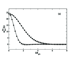
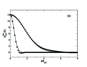
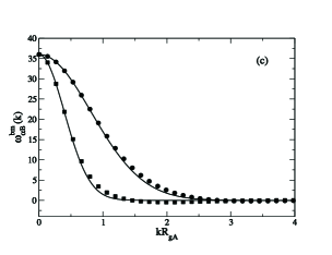
Figure 1:

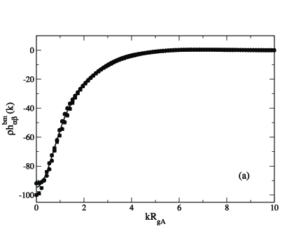
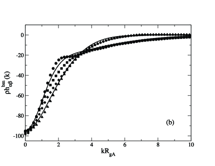
Figure 2:

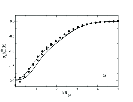
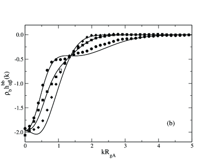
Figure 3:

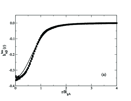
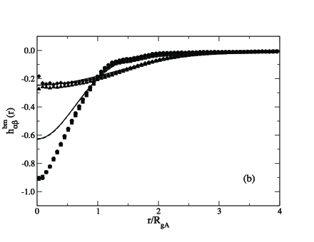
Figure 4:

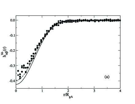
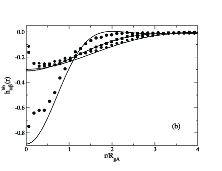
Figure 5:

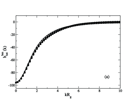
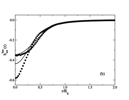
Figure 6:

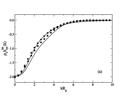
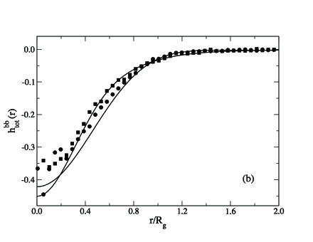
Figure 7:

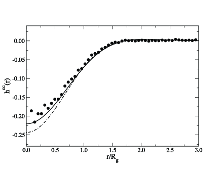
Figure 8:

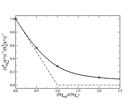
Figure 9:

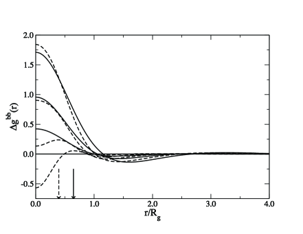
Figure 10:

References

- (1) J.-L. Barrat and J.-P. Hansen, Basic Concepts for Simple and Complex Liquids (Cambridge University Press, New York, 2003).
- (2) R. G. Larson, The Structure and Rheology of Complex Fluids (Oxford University Press, New York, 1999).
- (3) T. A. Witten and P. A. Pincus Structured Fluids (Oxford University Press, New York, 2004).
- (4) I. W. Hamley (Ed.) Developments in Block Copolymer Science and Technology (Wiley, Hoboken, New Jersey, 2004).
- (5) N. P. Balsara and M. J. Park, J. Pol. Sci. B: Pol. Phys. 4, 3429 (2006).
- (6) D. Frenkel and B. Smith Understanding Molecular Simulations: from Algorithms to Applications (Academic Press, San Diego, California, 2002).
- (7) M. Karttunen, I. Vattulainen, and A. Lukkarinen (Eds.) Novel Methods in Soft Matter Simulations, Lect. Notes Phys. 640 (Springer-Verlag, Berlin, 2004).
- (8) J. Dautenhahn and C. Hall, Macromolecules 27, 5399 (1994).
- (9) M. Murat and K. Kremer, J. Chem. Phys. 108, 4340 (1998).
- (10) F. Eurich and P. Maass, J. Chem. Phys. 114, 7655 (2001).
- (11) P. Kindt and W. J. Briels, J. Chem. Phys. 123, 224903 (2005).
- (12) V. Krakoviack, J.-P. Hansen, and A. A. Louis, Europhys. Lett. 58, 53 (2002).
- (13) V. Krakoviack, J.-P. Hansen, and A. A. Louis, Phys. Rev. E 67, 041801 (2003).
- (14) V. Krakoviack, B. Rotenberg, and J.-P. Hansen, J. Phys. Chem. B 108, 6697 (2004).
- (15) P. G. Bolhuis, A. A. Louis, J.-P. Hansen, and E. J. Meijer, J. Chem. Phys. 114, 4296 (2001).
- (16) P. G. Bolhuis, A. A. Louis, and J.-P. Hansen, Phys. Rev. E 64, 021801 (2001).
- (17) G. Yatsenko, E. J. Sambriski, M. A. Nemirovskaya, and M. Guenza, Phys. Rev. Lett. 93, 257803 (2004).
- (18) E. J. Sambriski, G. Yatsenko, M. A. Nemirovskaya, and M. G. Guenza, J. Chem. Phys. 125, 234902 (2006).
- (19) E. J. Sambriski, G. Yatsenko, M. A. Nemirovskaya, and M. G. Guenza, J. Phys.: Condens. Matter 19 205115 (2007).
- (20) G. Yatsenko, E. J. Sambriski, and M. G. Guenza, J. Chem. Phys. 122, 054907 (2005).
- (21) Y. Tsori, and D. Andelman, J. Pol. Sci. B: Pol. Phys. 44, 2725 (2006).
- (22) D. Reith, M. Ptz, F. Mller-Plathe, J. Comput. Chem. 24, 1624 (2003).
- (23) X. Li, D. Kou, S. Rao, aand H. Liang, J. Chem. Phys. 124, 204909 (2006).
- (24) C. Pierleoni, C.I. Addison, J.P. Hansen, and V. Krakoviack Phys. Rev. Lett. 96, 128302 (2006).
- (25) C. I. Addison, J. P. Hansen, V. Krakoviack, and A. A. Louis, Mol. Phys. 103, 3045 (2005).
- (26) J.P. Hansen and C.J. Pearson, Mol. Phys. 104, 3389 (2006).
- (27) K. S. Schweizer and J. G. Curro, Chem. Phys. 149, 105 (1990).
- (28) E. F. David and K. S. Schweizer, J. Chem. Phys. 100, 7767 (1994).
- (29) E. F. David and K. S. Schweizer, J. Chem. Phys. 100, 7784 (1994).
- (30) L. Leibler, Macromol. 13, 1602 (1980).
- (31) M. W. Matsen and F. S. Bates, Macromol. 29, 1091 (1996).
- (32) M. W. Matsen and M. Schick Curr. Opin. Colloid Interface Sci. 1, 329 (1996).
- (33) C.N.Likos, Phys. Rep. 348, 267 (2001).
- (34) J.-P. Hansen and I. R. McDonald, Theory of Simple Liquids (Academic Press, London, 1991).
- (35) G. H. Fredrickson and E. Helfand, J. Chem. Phys. 87, 697 (1987)
- (36) S. A. Brazovskii, Sov. Phys. JETP 41, 85 (1975).
- (37) M. Guenza and K. Schweizer, J. Chem. Phys. 106, 7391 (1997).
- (38) M. Guenza and K. S. Schweizer, Macromol. 30, 4205 (1997).
- (39) M. Guenza, H. Tang, and K. S. Schweizer, J. Chem. Phys. 108, 1257 (1998).
- (40) M. Guenza and K. S. Schweizer, J. Chem. Phys. 108, 1271 (1998).
- (41) K. S. Schweizer and J. G. Curro, Adv. Polym. Sci. 116, 319 (1994).
- (42) T. Ohta and K. Kawasaki, Macromolecules 19, 2633 (1996).
- (43) G. H. Fredrickson, Macromol. 20, 2535 (1987).
- (44) M. Doi and S. F. Edwards, The Theory of Polymer Dynamics (Oxford University Press, Oxford, 1986).
- (45) H. Yamakawa, Modern Theory of Polymer Solutions (Harper and Row, New York, 1971).
- (46) E. Jaramillo, D. T. Wu, G. S. Grest, and J. G. Curro, J. Chem. Phys. 120, 8883 (2004).