Magnetic processes in a collapsing dense core. I Accretion and Ejection

Abstract

Context. It is important for the star formation process to understand the collapse of a prestellar dense core.

Aims. We investigate the effect of the magnetic field during the first collapse up to the formation of the first core, focusing particularly on the magnetic braking and the launching of outflows.

Methods. We perform 3D AMR high resolution numerical simulations of a magnetically supercritical collapsing dense core using the RAMSES MHD code and develop semi-analytical models that we compare with the numerical results.

Results. We study in detail the various profiles within the envelope of the collapsing core for various magnetic field strengths. Even modest values of magnetic field strength modify the collapse significantly. This is largely due to the amplification of the radial and toroidal components of the magnetic field by the differential motions within the collapsing core. For a weak magnetic intensity corresponding to an initial mass-to-flux over critical mass-to-flux ratio, $\mu$ equals to 20, a centrifugally supported disk forms. The strong differential rotation triggers the growth of a slowly expanding magnetic tower. For a higher magnetic field strengths corresponding to $\mu=2$, the collapse occurs primarily along the field lines, therefore delivering weaker angular momentum in the inner part whereas at the same time, strong magnetic braking occurs. As a consequence no centrifugally supported disk forms. An outflow is launched from the central thermally supported core. Detailed comparisons with existing analytical predictions indicate that it is magneto-centrifugally driven.

Conclusions. For cores having a mass-to-flux over critical mass-to-flux radio $\mu<5$, the magnetic field appears to have a significant impact. The collapsing envelope is denser and flatter than in the hydrodynamical case and no centrifugally supported disk forms. For values $\mu<20$, the magnetic field drastically modifies the disk evolution. In a companion paper, the influence of the magnetic field on the dense core fragmentation is studied.

1 Introduction

Studying the collapse and the fragmentation of a protostellar molecular dense core is of great relevance for the star formation process. While the role of the magnetic field has long been suspected (e.g. Shu et al. 1987), it is still a disputable issue.

The first calculations of a collapsing dense core were monodimensional and treated ambipolar diffusion (e.g. Ciolek & Mouschovias 1994, Basu & Mouschovias 1995). Their main goal was to investigate the role of the magnetic support in delaying the protostar formation. At about the same time, a few attempts were made to calculate the collapse in 2 or even 3D (Phillips & Monaghan 1985, Fiedler & Mouschovias 1992). In parallel to the numerical efforts, various authors have looked for analytical solutions of this problem (Galli & Shu 1993ab, Nakamura et al. 1995, Li & Shu 1996, Basu 1997, Krasnopolsky & Königl 2002, Hennebelle 2003, Tilley & Pudritz 2003).

With the increasing computing power and the improvement of the numerical schemes, recent developments have been realized and various 2D (Nakamura et al. 1995, Tomisaka 1998, Allen et al. 2003) as well as 3D numerical calculations have been performed (Hosking & Whitworth 2004, Machida et al. 2005, 2007, Ziegler 2005, Banerjee & Pudritz 2006, Fromang et al. 2006, Price & Bate 2007).

In these calculations, it has been found that the magnetic field plays a crucial role in the evolution of the collapsing dense core, in particular in the context of fragmentation in multiple systems. It has also been found that outflows can be spontaneously launched during the collapse. These outflows have strong similarities with the one studied in many papers either numerically (e.g. Uchida & Shibata 1985, Casse & Keppens 2003, Pudritz et al. 2007) or analytically (e.g. Blandford & Payne 1982, Pelletier & Pudritz 1992, Contopulos & Lovelace 1994, Ferreira 1997).

Here, we present further 3D numerical calculations of a collapsing magnetised dense core. Our main goals are to investigate the influence of the magnetic field strength on the collapsing envelope, the disk and the outflows. The fragmentation is studied in a companion paper (Hennebelle & Teyssier 2007, hereafter paper II). In order to identify the physical mechanisms at play, we develop various analytical approaches that we then compare with the numerical solutions. The outline of the paper is as follow. In the second part, the numerical setup and the initial conditions are presented. The third part studies the evolution of the envelope. For this purpose, semi-analytical solutions are obtained and compared with the numerical results. The fourth part presents the results for the outflows. Comparison with classical analytical results are made. In the fifth part, we qualitatively compare our results with various observations, focussing particularly on the young class 0 source, IRAM04191 (André et al. 1999, Belloche et al. 2002) The sixth part concludes the paper.

2 Numerical setup and initial conditions

We perform 3D numerical simulations using the AMR code RAMSES (Teyssier 2002, Fromang et al. 2006). RAMSES is based on shock capturing schemes and can handle ideal MHD, self-gravity and cooling. It uses the constraint transport method to update the magnetic field and therefore is preserving the nullity of the divergence of the magnetic field. RAMSES has been widely tested and gives results comparable to other MHD codes for a large set of benchmarks. The AMR scheme offers access to the high resolution needed to treat the problem. All the calculations performed in the following use the Roe solver.

The calculations start with initially $64^{3}$ grid cells. As the collapse proceeds, new cells are introduced in order to ensure that the Jeans length is described everywhere with at least 10 cells. Nine levels of AMR are used for a total of about 10⁶ grid cells and an equivalent numerical resolution of $16384^{3}$.

Here, we consider simple initial conditions, namely an initially uniform sphere in solid body rotation. The magnetic field is initially uniform and parallel to the rotation axis. The sphere is embeded into a diffuse medium hundred times less dense. This makes that the surface of the cloud is initially out of pressure equilibrium and therefore expanding. However, since the cloud as a whole, is strongly self-gravitating, the collapse is not affected. The motivation to start with such simple conditions, sometimes considered as the standard test case for gravitational collapse of dense cores, instead of, for example, with a quasi-equilibrium configuration, is twofold. First, the magnetised collapse has not been widely explored yet and we feel it is important at this stage to choose conditions which can be easily reproduced by others. Second, unlike in the hydrodynamical case, when magnetic field and rotation are considered, the age of the structure does influence the angular momentum distribution and the structure of the field lines. This makes the choice of starting with such a structure in near equilibrium also questionable.

Initially, the ratio of the thermal over gravitational energy, $\alpha$, is about 0.37 whereas the ratio of rotational over gravitational energy, $\beta$, is equal to 0.045. These values are comparable to standard values quoted in various studies of dense cores and are not too far from typical values inferred from observations. The cloud temperature is equal to 11 K. The cloud has a mass of one solar mass, a radius of about $R_{0}\simeq$0.016 pc, a density $\simeq 5\times 10^{-18}$ g cm^-3 giving a freefall time, $\tau_{ff}\simeq 3\times 10^{4}$ years. In the companion paper (paper II), an $m=2$ perturbation of various amplitudes is added.

The strength of the magnetic field is expressed in terms of mass-to-flux over critical mass-to-flux ratio, $\mu=(M/\Phi)/(M/\Phi)_{c}$, where $(M/\Phi)_{c}=c_{1}/3\pi\times(5/G)^{1/2}$ (Mouschovias & Spitzer 1976) and $\Phi$ is the magnetic flux. $c_{1}$ has been estimated to be about 0.53. The case $\mu=1$ corresponds to a cloud just magnetically supported, i.e. magnetic forces balance gravitational forces. Various magnetic strengths are considered in the following, namely, $\mu=1000$ (quasi-hydrodynamical case), $\mu=20$ (very supercritical cloud), $\mu=5$ and $\mu=2$ (highly magnetised super critical cloud).

In order to avoid the formation of a singularity and to mimic the fact that at very high density, the dust becomes opaque and therefore the gas becomes nearly adiabatic, we use a barotropic equation of state: $C_{s}^{2}=(C_{s}^{0})^{2}\times(1+(\rho/\rho_{c})^{4/3})^{1/2}$, where $C_{s}\simeq 0.2$ km/s is the sound speed and $\rho_{c}=10^{-13}$ g cm^-3. Note that Masunaga & Inutsuka (2000) demonstrate that this is a good approximation for a one solar mass core.

However, with such an equation of state, the timestep in the central part of the cloud becomes so small that it is difficult to follow the collapse during a long period of time. In order to avoid that problem, we have also performed complementary simulations with a critical density $\rho_{c}/10=10^{-14}$ g cm^-3.

3 Envelope evolution

In this section, we study the properties of the various fields in the collapsing envelope. We first present our notations and a simple semi-analytical approach which will be useful to understand the simulation results.

3.1 Analytical model

Here, we develop a phenomenological model for the profiles of the various fields near the equatorial plane. We stress that the main motivation in carrying out such analysis is to have models to interpret more accurately the complex numerical results. More elaborate models have been developed (e.g. Galli & Shu 1993ab, Li & Shu 1996, Krasnopolsky & Königl 2002) assuming mainly self-similarity or equilibrium. Since both are restrictive assumptions and given the complexity of the numerical results obtained in the following, it is unclear to which extent these models could be used for the purpose of comparison although they undoubtedly provide a sensible hint on the physical processes.

3.1.1 Notation and assumptions

We consider an initially uniform cloud of mass $M_{0}$, initial radius $R_{0}$, in solid body rotation with angular velocity $\omega_{0}$ and threaded by a uniform magnetic field $B_{z}^{0}$ parallel to the z-axis.

In the following, we use standard Cartesian coordinates $(x,y,z)$ and cylindrical coordinates $(r,\theta,z)$ therefore $r=\sqrt{x^{2}+y^{2}}$.

Let $h$ be the scale height of the cloud near the equator, we write (see e.g. Li & Shu 1996):

$$h(r)=a\times r,$$

$$\rho(r)={dC_{s}^{2}\over 2\pi Gr^{2}},$$ (1)

$$B_{z}(r)={H_{z}C_{s}^{2}\over\sqrt{G}r},$$

where $\rho$ and $B_{z}$ are the density and z-component of the magnetic field near the equator respectively. In the following, it will be assumed that $a$, $d$ and $H_{z}$ depend weakly on $r$. It is well known that such scaling is a reasonable approximation in the envelope during the class-0 phase in particular before the rarefaction wave launched at the formation of the protostar has propagated significantly (Shu 1977).

The structures of the radial and azimuthal components of the magnetic field are a little more complex. It is well known that for symmetry reasons, $B_{r}$ and $B_{\theta}$ vanish in the equatorial plane, $z=0$. Their values increase with $z$ until they reach their maximum, after which they decrease with $z$. Since here we are interested only in the value near the equatorial plane, we write as Krasnopolsky & Königl (2002)

$$B_{r}(r,z,t)=H_{r}(r,t)\times{z\over h(r)}{C_{s}^{2}\over\sqrt{G}r},$$ (2)

$$B_{\theta}(r,z,t)=H_{\theta}(r,t)\times{z\over h(r)}{C_{s}^{2}\over\sqrt{G}r}.$$

These two expressions are valid until $z\simeq h$. At higher altitude, $B_{r}$ and $B_{\theta}$ decrease and tend toward their value outside the core which in the present simulations is zero. Therefore, it is expected that the values of $|B_{r}|$ and $|B_{\theta}|$ at a given radius, $r$, are maximum at the altitude, $z\simeq h(r)$, ${\rm max}(B_{r}(r,z))\simeq H_{r}C_{s}^{2}/\sqrt{G}r$ and ${\rm max}(B_{\theta}(r,z))\simeq H_{\theta}C_{s}^{2}/\sqrt{G}r$.

Thus, in the following, it seems appropriate to display the quantities ${\rm max}(B_{r}(r,z))/B_{z}(r,0)=H_{r}/H_{z}$ and ${\rm max}(B_{\theta}(r,z))/B_{z}(r,0)=H_{\theta}/H_{z}$.

3.1.2 Axial and radial components of the magnetic field

Since throughout this work, field freezing is assumed, the magnetic flux, $\Phi$, is conserved within the cloud. Therefore:

$$\Phi=\int B_{z}\times 2\pi rdr=B_{z}^{0}\times\pi R_{0}^{2}=2\pi H_{z}(C_{s}^{2}/\sqrt{G})R_{c},$$ (3)

where $R_{c}$ is the cloud radius at the current time whereas $R_{0}$ is the initial cloud radius. Thus we have:

$$H_{z}=(\sqrt{G}/C_{s}^{2})\times B_{z}^{0}R_{0}^{2}/(2R_{c}).$$ (4)

Note that in this expression the cloud radius $R_{c}$ is not known. With our choice of initial conditions, $R_{c}$ does not evolve much during the class-0 phase and we will assume $R_{c}\simeq R_{0}$ in the following. This leads to

$$B_{z}(r)=\frac{B_{z}^{0}}{2}\frac{R_{0}}{r}$$ (5)

The $r$-component is less straightforward to obtain. Its growth is due to the stretching of the field lines by the differential motions within the cloud. In the case of a thin and isopedic disk, Li & Shu (1997) demonstrated that the magnetic flux and gravitational potential are proportional through the cloud allowing one to compute all components of the magnetic field once the gravitational potential is known. Krasnopolsky & Königl (2002) have assumed that $B_{r}$ is simply proportional to the magnetic flux. Since the $B_{r}$ component appears difficult to predict quantitatively, we simply write

$$H_{r}=\eta H_{z}$$ (6)

and the value of $\eta$ will be estimated from the simulation.

3.1.3 Density field

In order to estimate the density, we write axial and radial equilibrium conditions. Although the cloud is not exactly in equilibrium since it is collapsing, such assumptions lead nevertheless to reasonable estimates of the density as long as the collapse is not strongly triggered (Shu 1977, Hennebelle et al. 2003).

The equilibrium along the z-axis, neglecting the azimuthal component of the magnetic field and the tension term $B_{z}\partial_{r}B_{r}$, is:

$$-C_{s}^{2}\partial_{z}\rho+\rho\partial_{z}\psi-\partial_{z}\left({B_{r}^{2}\over 8\pi}\right)=0,$$ (7)

where $\psi$ is the gravitational potential. Integrating once, we obtain (using $\partial_{z}^{2}\psi\simeq-4\pi G\rho$):

$$C_{s}^{2}\rho+{1\over 8\pi G}(\partial_{z}\psi)^{2}+{B_{r}^{2}\over 8\pi}=K(r),$$ (8)

where $K(r)$ is a function of $r$. Evaluating $K$ at $z=0$ and at $z=h$, and using the expressions stated by Eqs. (1) and (4), we get

$$d\simeq d^{2}a^{2}+{\eta^{2}\over 4}H_{z}^{2},$$ (9)

where we have also used the approximation $\partial_{z}\psi\simeq-4\pi G\rho h$.

The equilibrium along the radial direction is (neglecting again the influence of $B_{\theta}$)

$$-C_{s}^{2}\partial_{r}\rho+{1\over 4\pi}(-B_{z}\partial_{r}B_{z}+B_{z}\partial_{z}B_{r})+\rho\partial_{r}\psi\simeq 0.$$ (10)

Thus we obtain, with Eqs. (1) and (2)

$$d+{H_{z}^{2}\over 4}(1+\eta/a)\simeq ad^{2},$$ (11)

where the gravitational force $\partial_{r}\psi$ has been assumed to be $\partial_{r}\psi\simeq-GM/r^{2}$ with $M\simeq\int 2\pi r\times 2h(r)\rho dr$.

$H_{z}$ being known from Eq. (4), Eqs. (9) and (11) can be solved numerically once $\eta$ is estimated from the simulation, to provide the values of $d$ and $a$. For the case $H_{z}=0$, we have $a=d=1$, i.e. the structure of the cloud is not modified by the magnetic field and therefore the density is the Singular Isothermal Sphere (SIS) density (since the analytical model does not consider the effect of rotation).

3.1.4 Azimuthal magnetic field and rotation

The azimuthal component of the magnetic field, as well as the rotation are more difficult to obtain. In order to do so, we adopt a Lagrangian approach, i.e. we follow the fluid particle and compute its momentum and azimuthal magnetic field along time. For this purpose, we simply use the fluid equations with density and poloidal field given as described above. To use dimensionless quantities, we define

$$\widetilde{r}=r/R_{0},\widetilde{M}=M(r)/M_{0},\widetilde{t}=t\times\sqrt{GM_{0}/R_{0}^{3}}$$ (12)

To compute the position of the fluid particle, we simply write (neglecting the thermal pressure)

$$d_{t}V_{r}\simeq-{G_{\rm eff}M(r_{0})\over r^{2}}+{V_{\theta}^{2}\over r}$$ (13)

with $V_{r}=dr/dt$. In this expression, $M(r_{0})$ is the mass of the cloud within a radius $r_{0}$ and $G_{\rm eff}$ is the effective gravitational constant $G_{\rm eff}=G\times(1-1/\mu)$. It will be assumed that $M$ remains constant during the collapse, i.e. we do not consider any accretion which may arise along the pole. Thus, we obtain

$$d_{\widetilde{t}}\widetilde{V}_{r}\simeq-{\widetilde{M}(r_{0})\over\widetilde{r}(\widetilde{t})^{2}}+{L(\widetilde{t})^{2}\over\widetilde{r}(\widetilde{t})^{3}}$$ (14)

where $L=\widetilde{r}\widetilde{V}_{\theta}$ is the momentum of the fluid particle.

The momentum equation is

$$d_{t}(rV_{\theta})={1\over 4\pi\rho}(B_{r}\partial_{r}(rB_{\theta})+rB_{z}\partial_{z}B_{\theta})$$ (15)

Gathering Eqs. (1), (2) and (12), we get

$$d_{\widetilde{t}}L\simeq K\times{H_{z}H_{\theta}(t)\over ad},$$ (16)

where $K=C_{s}^{2}R_{0}/(2GM_{0})$.

Finally, the induction equation together with Eqs. (1) and (2) leads to

$$d_{\widetilde{t}}H_{\theta}\simeq-\eta{L(\widetilde{t})H_{z}\over\widetilde{r}(\widetilde{t})^{2}}$$ (17)

Once $a$ and $d$ are known, Eqs. (14), (16) and (17) can be integrated with time to obtain the particle momentum. In the following, we use these equations to directly compare with the numerical results.

Figure 1: Case $\mu=1000$. Density (left-top), radial (left-middle) and azimuthal velocity (left-bottom) and z-component of magnetic field (right-top) in the equatorial plane at different times. Largest values of the radial (right-middle) and azimuthal (right-bottom) magnetic components at a given radius are also given. For convenience, ${\rm max}(B_{r}(r,z))/B_{z}(r,0)$ and ${\rm max}(B_{\theta}(r,z))/B_{z}(r,0)$ are given as a function of $r$. The various straight lines show analytical values (see text).

Figure 2: Same as Fig. 1 for case $\mu=20$.

Figure 3: Same as Fig. 1 for case $\mu=5$.

Figure 4: Same as Fig. 1 for case $\mu=2$.

3.2 Cloud radial profiles

Figures 1-4 show the density, radial velocity, rotation velocity and z-component of the magnetic field in the equatorial plane (variations along the z-axis are shown in Sect. 4 ) as a function of radius for various magnetic field strengths. They also display the largest value of radial and azimuthal components of the magnetic field at a given radius. These values are obtained by taking the largest values along the z-axis at each radius. Note that as recalled in the previous section, $B_{r}$ and $B_{\theta}$ vanish in the equatorial plane $z=0$. Therefore, the maximum value of $B_{r}(r,z)/B_{z}(r,0)$ at a given $r$ is plotted. Four snapshots are displayed. The first one is representative of the prestellar phase and is about 0.06-0.08$\times\tau_{\rm ff}$ before density reaches the critical density, $\rho_{c}$, the second one is near the time at which the density reaches $\rho_{c}$ whereas the third and fourth ones show latter evolution. The two straight solid lines in the density plots show the density of the singular isothermal sphere (lower lines) and the density of the analytical model stated by Eq. (1) (upper lines). Note that in the hydrodynamical case, the two straight lines are indistinguishable. Table 1 gives the values of the parameters, $\mu$, $H_{z}$, $\eta$, $a$ and $d$. The straight solid lines in the $B_{z}$ plots show the analytical estimate of $B_{z}$ stated by Eq. (1) and (4).

Table 1: Values for the parameters. $\eta$ is estimated from the numerical simulation. $H_{z}$, $a$ and $d$ are obtained from the analytical model.

$\mu$	$H_{z}$	$\eta$	$a$	$d$
20	0.41	5	0.48	2.48
5	1.64	3	0.2	10.29
2	4.10	2	0.12	29.37

3.2.1 Quasi-hydrodynamical case

Figure 1 shows results for $\mu=1000$, i.e. quasi-hydrodynamical case. The density is slightly stiffer than $r^{-2}$ in the outer part where it is a little denser than the SIS. This is due to the rotation and to the fact that the cloud is collapsing and therefore not in equilibrium (Shu 1977, Hennebelle et al. 2003, 2004a). In the inner part of the envelope the ratio of density over SIS density increases even more with radius. This is due to the rotation velocity which increases with $r$ (Ulrich 1976). Note that a better agreement between analytical and numerical estimate can be obtained by taking into account the influence of rotation in the former (see e.g. Hennebelle et al. 2004a). Two accretion shocks are visible in the radial velocity plot. The first one which is located at $r=10^{-3}$ pc shows the edge of the centrifugally supported disk. The second one, located at $r=10^{-4}$ pc, shows the edge of the thermally supported core. Although for this case, the magnetic field has almost no influence on the gas dynamics, it is worth studying the spatial dependence of the three components. The $B_{z}$ component in the envelope appears to be reasonably close to the analytical estimate stated by Eq. (1), the discrepancy being due to the fact that $\rho$ is stiffer than $r^{-2}$ because of rotation. The $B_{r}$ and $B_{\theta}$ components which vanish initially, have slightly different behaviour. They grow with time and reach values of the order of $B_{z}$ in the outer part of the envelope down to values roughly 10-100 times larger than $B_{z}$ at the edge of the disk. Inside the centrifugally supported disk these values increase further up to values as high as about $10^{3}$. It should be noted however that here we are plotting the maximum values of $B_{r}$ and $B_{\theta}$ at a given radius. Since in the case $\mu=1000$, the disk quickly fragments (see paper II), $B_{r}$ and $B_{\theta}$ fluctuate significantly and therefore the high values reached in the inner parts are much higher than the mean values of $B_{r}$ and $B_{\theta}$ (see paper II for an estimate of their mean values in the disk). Note also that the increase of ${\rm max}(B_{r})/B_{z}$ and ${\rm max}(B_{\theta})/B_{z}$ at large radius ($r>10^{-2}$ pc) is simply due to the decrease of $B_{z}$ in the external medium surrounding the cloud.

3.2.2 Weak field case

Figure 2 shows results for $\mu=20$, i.e. weakly magnetised case. As expected, since the magnetic field is weak, the density, radial and azimuthal velocity fields are very close to those obtained in the previous case. $B_{z}$ is much larger than in the case $\mu=1000$. As for the previous case, the values of ${\rm max}(B_{r})/B_{z}$ and ${\rm max}(B_{\theta})/B_{z}$ increase gradually in the envelope. They reach values of roughly 10 at the edge of the disk. This indicates that the differential motions within the cloud are less important in this case because of the influence of the Lorentz force. As in the hydrodynamical case, a centrifugally supported disk formed as well as two accretion shocks. Note again that the large fluctuations of $B_{r}$ and $B_{\theta}$ within the disk are due to the display of the maximum of $B_{r}$ and $B_{\theta}$ at a given radius. As shown in paper II, some symmetry breaking is occurring in the disk which generates strong fluctuations.

3.2.3 Intermediate field cases

Figures 3 and 4 respectively show results for $\mu=5$ and $\mu=2$, i.e. intermediate and strongly magnetised supercritical cases. The density and velocity fields are significantly different from the two preceding cases. The equatorial density is roughly 10 to 30 times the density of the SIS and is in good agreement with the analytical estimate stated by Eq. (1). This is mainly due to the magnetic pressure (due to $B_{r}$) which compresses the gas along the z-axis. In the outer part, the radial velocities are smaller than in the weak field cases. This is due to the influence of the Lorentz force which supports the cloud. On the contrary, in the inner part, the radial velocities are larger than in the weak field cases. This is because, since the rotation is much smaller than in the weak field case, the centrifugal support is much weaker. In the case $\mu=5$, a weak local maximum, due to the centrifugal force is nevertheless still present at $r\simeq 2-3\times 10^{-4}$ pc. However, unlike in the cases $\mu=1000$ and 20, the radial velocity does not vanish except in the center. This indicates that there is no real centrifugally supported disk in this case. For $\mu=2$, only the shock on the thermally supported core remains, indicating that the centrifugal force is not able to stop the gas. The reason for lower angular momentum will be analyzed in the next section. We note that similar conclusions have been recently reached by Mellon & Li (2007). It is also apparent that the shape of the rotation velocity is flatter when $\mu$ is smaller: the rotation curve stays roughly constant until much smaller radii.

The z-component of the magnetic field is very close to the analytical estimate in the envelope of the core. The value of ${\rm max}(B_{r})/B_{z}$ is about 2 at the edge of the core for $\mu=5$ and about 1 for $\mu=2$. It gradually increases inwards and reaches values about 2-3 times larger in the inner part. The values of ${\rm max}(B_{\theta})/B_{z}$ are typically 1.5 to 2 times smaller than ${\rm max}(B_{r})/B_{z}$ for $\mu=5$ and about 3 times for $\mu=2$.

Altogether these results illustrate that even for low to intermediate values of the magnetic strength, magnetic field can have a drastic influence on the cloud evolution as well as on the disk formation. This is due to the fact that the radial and toroidal components of the magnetic field, which vanish initially, are strongly amplified during the collapse by the differential motions. This makes that the radial component $B_{r}$ does not increase linearly with the initial magnetic field strength since the field is easier to stretch when it is initially weaker.

It is worth stressing that such values of $\mu$ in the range $5-2$ are compatible with the more pessimistic estimates derived from measurements of the magnetic intensity in the dense cores (Crutcher 1999, Crutcher & Troland 2000, Crutcher et al. 2004). Since we find that dense cores having $\mu$ smaller than $\simeq$5 are qualitatively different from the hydrodynamical cores, we conclude that magnetic fields are playing an important role in the collapse of dense cores and therefore in the star formation process.

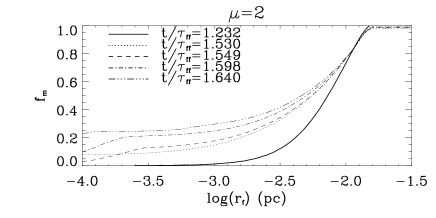
Figure 5: Fraction of cloud mass, $f_{m}$, enclosed within a cylinder of radius, $r_{f}$, as a function of $r_{f}$. Upper panel is case $\mu=20$. Lower panel is case $\mu=2$.

Figure 6: Mean specific angular momentum enclosed within a cylinder of radius, $r_{f}$, containing a cloud mass fraction $f_{m}$, as a function of $f_{m}$. Upper panel is case $\mu=20$. Lower panel is case $\mu=2$.

Figure 7: Case $\mu=20$. Specific angular momentum of the fluid particle located at cloud radius, $r_{f}$, where $r_{f}$ is the radius of the cylinder enclosing a constant mass fraction $f_{m}$. Each point corresponding to a given time, this diagram shows the time evolution of the angular momentum of the fluid particle as the collapse proceeds. The solid lines correspond to the analytical model presented in Sect. 3 (see text). The dashed lines show the radius of the magnetized area which surrounds the thermally supported core, below which the analytical model is not appropriate.

Figure 8: Same as Fig. 7 for case $\mu=2$.

3.3 Angular momentum evolution

Here, we further study the radial distribution of angular momentum. In particular, we investigate the physical origin of smaller rotation velocities in the intermediate and strong field cases.

3.3.1 Mass and angular momentum distribution

For this purpose, we plot the fraction of mass, $f_{m}$, enclosed inside cylinders of various radii for the cases $\mu=20$ and $\mu=2$ in Fig. 5. Note that the first two times correspond to a critical density equal to $\rho_{c}$, whereas for the three others, the critical density is $\rho_{c}/10$. As can be seen, a good agreement is obtained between the second and the third times which are close in time, showing that varying the critical density does not affect significantly the envelope evolution. We define the radius $r_{f}$ of the cylinder containing a constant mass fraction $f_{m}$. $r_{f}$ decreases with time as the collapse proceeds.

Comparison between the 2 panels of Fig. 5 reveals that the mass distribution as a function of radius is significantly different in the two cases $\mu=20$ and $\mu=2$. In particular, the mass fraction enclosed within a cylinder of radius $\simeq 3\times 10^{-3}$ pc is roughly fifty percent higher for $\mu=20$ than for $\mu=2$. This indicates that the collapse arises in different ways for these two cases. In fact, the collapse is more spherical for $\mu=20$ than for $\mu=2$. In the latter, since the field is strong, the collapse first proceeds along the field lines implying that the material which constitutes the central core and the disk was originally located closer to the rotation axis than for the case $\mu=20$. Since material close to the rotation axis has a lower angular momentum than the gas located further away, we believe that this is one of the reason of lower angular momentum in the cloud central parts in the case $\mu=2$ than in the case $\mu=20$.

Figure 6 displays the distribution of mean specific angular momentum within a cylinder enclosing a mass fraction $f_{m}$ as a function of $f_{m}$. It shows that the specific angular momentum for the first two times are both proportional to the mass fraction and that the cloud with $\mu=20$ has a specific angular momentum which is only 20$\%$ higher than for the case $\mu=2$. This difference which is attributable to the magnetic braking, shows that magnetic braking plays only a minor role during the early parts of the collapse. Fig. 6 together with Fig. 5 also demonstrates that the total angular momentum in the case $\mu=20$ is higher in the internal part of the cloud than in the case $\mu=2$. The subsequent times shown in these figures reveal that the specific angular momentum stays roughly constant indicating that magnetic braking remains rather inefficient in the case $\mu=20$. On the contrary, the subsequent times displayed in the second panel of Fig. 5 show that the specific angular momentum decreases drastically in the inner part of the cloud. This is most likely due to the magnetic braking. We stress however, that at time $t=1.53\tau_{ff}$, the angular momentum has decreased significantly only in the very inner part corresponding to $f_{m}<0.15$. With Fig. 6, we see that this corresponds to radii smaller than $10^{-3}$ pc. Therefore, the small rotation velocities seen in Fig. 4 are largely due to the collapse proceeding first along the field lines. At this time, magnetic braking has efficiently reduced the gas angular momentum in the very inner parts only.

3.3.2 Comparison between analytical and numerical results

In order to compare the numerical results with the analytical model and to confirm that the decrease of angular momentum seen for $\mu=2$ is due to magnetic braking, we have calculated the specific angular momentum of the fluid particle located at the radius, $r_{f}$, where $r_{f}$ is the radius of the cylinder which contains a cloud mass fraction $f_{m}$. Indeed, Fig. 6 shows that the mean angular momentum enclosed within a cylinder of radius $r_{f}$ does not vary much with time (except for the 2 last times displayed for $\mu=2$). This implies that the mass enclosed within radius $r_{f}$, does not vary significantly along time. Therefore, the selected fluid particle located at $r_{f}$ should remain nearly the same. Consequently, any angular momentum variation is attributable to magnetic braking. Figures 7 and 8 show, for different values of $f_{m}$, the specific angular momentum of the fluid particle as a function of radius at ten different times. It also displays analytical curves performed with the model presented in Sect. 3.1.4. To obtain these curves, we start with values of $r(t)$ and $L(t)$ corresponding to the first point shown in each panel of Figs. 7 and 8, and we integrate Eqs. (14), (16) and (17) using the values of $a$ and $d$ provided by Eqs. (9) and (11). Note that in order to mimic the growth of $B_{r}$ and the fact that it is initially zero, we use $\eta=\eta_{0}\times(1-r(t)/r(0))$ in Eq. (17). Since as shown in Fig. 2, the value of $\eta_{0}$ varies through the cloud, we run three models for $\eta_{0}$=1, 1.5 and 2. The top curves of Fig. 8 correspond to $\eta_{0}=1$ whereas the bottom curves correspond to $\eta_{0}=2$.

The ten times represented in the case $\mu=20$ correspond to 1, 1.15, 1.19, 1.2, 1.26, 1.35, 1.46, 1.54, 1.6, 1.63$\tau_{ff}$, whereas for $\mu=2$, they correspond to 1.21, 1.41, 1.53, 1.52, 1.55, 1.57, 1.60, 1.62, 1.64, 1.68$\tau_{ff}$. Note that for both cases, the first three times have been obtained with the standard critical density whereas the seven others have been obtained with the critical density $\rho_{c}/10$. The good continuity shows that the results are not affected by the thermally supported core (except maybe for the last times).

In the case $\mu=20$, there is, as expected, hardly any variation of angular momentum. The only variation occurs for $f_{m}=0.1$ at radius smaller than $r=3\times 10^{-4}$ pc, i.e. after the fluid particle has reached the central thermally supported core. In the case $\mu=2$, magnetic braking is much more effective. A significant loss of angular momentum is observed for $f_{m}=0.1$, $f_{m}=0.2$ and $f_{m}=0.3$. In each case, the analytical fit is in reasonable agreement with the numerical value until the fluid particle reaches a strongly magnetised area surrounding the thermally supported core where the analytical solution becomes inappropriate. This agreement shows that the analytical model is reasonably accurate and that magnetic braking is responsible for the angular momentum decrease. Depending on the value of $f_{m}$, the angular momentum decrease during the collapsing phase can be larger, comparable or smaller than the angular momentum decrease once the fluid particle has reached the magnetised area which surrounds the thermally supported core. Note that the size of this area increases with time due to accumulation of magnetic flux. This is why fluid particles corresponding to bigger $f_{m}$ reach it at larger radii.

To summarize, we can say that for low magnetic strengths, magnetic braking is too small to play a significant role in the envelope. In the case of strong fields, the collapse first occurs along the field lines therefore delivering a low angular momentum in the inner region. At the same time, magnetic braking reduces the angular momentum of the collapsing envelope. Finally, strong magnetic braking occurs in the surrounding of the thermally supported core which is highly magnetised.

Figure 9: Case $\mu=20$. Density and velocity fields in the xz plane.

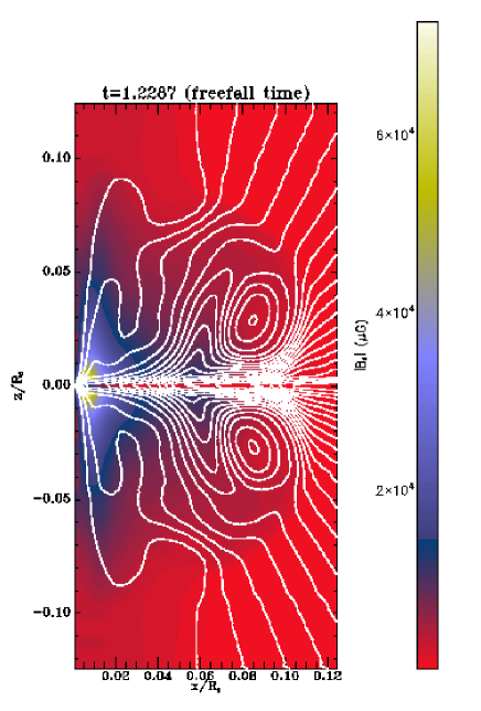
Figure 10: Structure of the azimuthally averaged magnetic field in the model having $\mu=20$ at time $t=1.2287\tau_{ff}$. The solid lines displays the poloidal magnetic field lines. They are overplotted on a snapshot of the toroidal magnetic field strength.

4 Outflows

It is now well known that accretion is often, maybe always, associated with ejection processes. In the context of star formation, molecular outflows as well as jets have been extensively observed (see e.g. Bally et al. 2007 for a recent review). While jets may have velocities as large as several hundred km s^-1, the bulk of the millimeter wavelength CO emission, tends to have velocities of only a few to ten km s^-1. In the following, we call outflows, outward motions with velocities larger than 1 km s^-1.

In this section, we study the various outflow motions obtained in these simulations. We first give a basic description of the weak and strong field cases. Then, a more detailed analysis is presented for each of these two cases. Finally, we show for both cases mass and angular momentum fluxes for long time evolution.

4.1 Weak field

Here we describe results for the case $\mu=20$.

4.1.1 Basic description

Figure 9 shows the density and velocity fields in the xz plane for $\mu=20$ at three times. A complex expanding structure forms around the center. As will be seen later, it is somehow similar to the magnetic tower investigated by Lynden-Bell (1996) and in the following we use this terminology. The first snapshot shows that this structure encompasses the centrifugally supported disk. As a consequence the accretion shock, which occurs near the equatorial plane in the hydrodynamical case, is located further away at the edge of the tower. At this stage, the tower is uniformly slowly expanding (see next section for quantitative estimates). The second snapshot shows that a faster outflow appears along the pole. It is clearly starting from the central thermally supported core. The velocity is all the way almost parallel to the z-axis. Since this outflow is faster than the surrounding slowly expanding tower, the shape of the structure becomes gradually more complex and mainly composed of two distinct regions, the faster flow and a slower magnetic tower. The third snapshot shows that this structure is maintained at later times without much change for the central flow whereas the tower keeps expanding. At the edges of the structure, near the equatorial plane, slow recirculation flows develop.

It should be noted at this stage that the thermal structure of the protostar is not correctly treated in this paper. In particular the second collapse is not considered here (Masunaga & Inutsuka 2000, Machida et al. 2007). Thus the central outflow may have a different structure in a more realistic simulation. Indeed, Banerjee & Pudritz (2006) and Machida et al. (2006, 2007) found that a fast outflow, maybe a jet, having velocities around 30 km/s develops during the formation of the protostar.

Figure 10 shows the structure of the magnetic field at time $t=1.2287\tau_{ff}$. The magnetic field is decomposed into its toroidal and poloidal parts, $B_{\theta}$ and ${\bf{B_{p}}}=(B_{r},0,B_{z})$. The strength of the former is shown using the colorscale snapshots while the poloidal magnetic field lines are represented using the solid white lines. The structure of the magnetic field appears to be complex. The field lines are strongly bent and twisted in the inner central regions ($x/R_{c}<0.1,\,|z/R_{c}|<0.1$) whereas they are almost straight in the outer part. In the same way, the toroidal component is 2 to 3 order of magnitude higher in the inner part than in the external part. This strongly suggests that the growth of the tower as well as the outflow are associated with the strong wrapping of the field lines. This effect is quantified in the following section.

Figure 11: Cut along the z-axis at $x/R_{c}=0.02$ and $y=0$ at four different times. Density, vertical component of the velocity, rotation velocity and toroidal component of the magnetic field are shown.

4.1.2 Quantitative estimates

Figure 11 shows the density, axial velocity, rotation velocity and toroidal component of the magnetic field along the z-axis for four times at $x/R_{0}=0.02$ and $y=0$. The first and second times (respectively solid and dotted lines) show that the central density is increasing due to the rapid accretion. Similarly, the angular momentum increases. The toroidal component of the magnetic field grows rapidly and is about 5 times larger at the second time than at the first. This induces a slow expansion at about 0.3-0.5 km/s.

The third time shows that the tower keeps expanding with about the same velocity and that the toroidal component of the magnetic field does not grow in intensity and saturates, forming a plateau (except close to $z=0$) with slowing decreasing value at high $z$. The total toroidal magnetic flux inside the structure increases since the size of this plateau increases.

To characterize the dynamical state of the tower, we estimate the thermal and magnetic pressure as well as the gravitational potential at $z\simeq 3\times 10^{-3}$ pc, i.e. close to the edge of the tower at time, $t=1.15\tau_{ff}$. The density is about $10^{-15}$ g cm^-3, giving a thermal pressure of about $5\times 10^{-7}$ erg cm^-3. The toroidal component of the magnetic field is about 10${}^{4}\mu G$ giving a magnetic pressure of about $B_{\theta}^{2}/8\pi\simeq 4\times 10^{-6}$ erg cm^-3. The gravitational force is less straightforward to estimate. By the time we are considering, the mass denser than $\simeq 10^{-15}$ g cm^-3 is of the order of $\simeq 0.1M_{s}$. Thus, the potential energy is of the order of $\simeq\rho GM/z\simeq 10^{-5}$ erg cm^-3. Therefore, we conclude that by the time $t=1.15\tau_{ff}$, the magnetic tower is largely dominated by the magnetic and the gravitational energies. At later times, as the expansion proceeds, the gravitational energy will eventually become negligible.

To assess that the expansion of the tower is indeed due to the growth of the toroidal magnetic field, we consider pressure equilibrium at the edge of the tower where we have

$$B_{\theta}^{2}/8\pi=\rho_{\rm inf}V_{\rm inf}^{2},$$ (18)

since the external pressure is dominated by the ram pressure, $\rho_{\rm inf}V_{\rm inf}^{2}$, exerted at the accretion shock.

The flux per unit length of the toroidal magnetic field, $\Phi_{\theta}$, is given by

$$\Phi_{\theta}=\int B_{\theta}dz\simeq B_{\theta}\times l,$$ (19)

$l$ being the height of the magnetic tower.

Integrating the induction equation along $z$, $\Phi_{\theta}$ is also given by

$$\Phi_{\theta}\simeq B_{z}V_{\theta}\times t,$$ (20)

where $B_{z}$ and $V_{\theta}$ are to be taken in the equatorial plane. Therefore, we obtain:

$$V_{\rm tower}\simeq{B_{z}\over\sqrt{8\pi\rho_{\rm inf}}}\times{V_{\theta}\over V_{\rm inf}}.$$ (21)

This expression is somehow similar to some of the expressions obtained by Lynden-Bell (1996, 2003) although his analysis is more sophisticated since the explicit value of the tower radius is taken into account. With $B_{z}\simeq 3\times 10^{3}\mu$G (obtained from Fig. 2), $V_{\theta}\simeq 0.9$ km/s, $V_{\rm inf}\simeq 1.3$ km/s and $\rho_{\rm inf}\simeq 3\times 10^{-17}$ g cm^-3 (obtained from Fig. 11 either at $z=0$ or at $z=9\times 10^{-4}$ pc), we obtain: $V_{\rm tower}\simeq 0.58$ km/s. This value is comparable with the value of $V_{z}\simeq 0.45$ km/s at time $t=1.15\tau_{ff}$ and $z=8\times 10^{-4}$ pc within about $25\%$. The difference is probably due to the assumption of constant $B_{\theta}$ in the tower. Note that this simple estimate does not take into account gravity. In order to investigate its influence, an analytical model for the expansion of the magnetic tower, is developed in the Appendix. Indeed, the model shows that the growth of the transverse magnetic field which is induced by the gradient of transverse velocity along the z-axis, triggers the expansion of a self-gravitating layer in a very similar way to what is observed in the simulation.

The last time in Fig. 11 shows that the z-velocity increases significantly and reaches values of about 1.2 km/s. This is due to the central outflow which presents higher velocities. At this stage the velocities of the tower and the flow are difficult to distinguish. The fourth time also reveals that angular momentum as well as mass have been removed probably by the outflow between $z=3\times 10^{-4}$ and $z=3\times 10^{-3}$ pc.

4.2 Strong field: magneto-centrifugal ejection

Here we describe results for the case $\mu=2$.

Figure 12: Case $\mu=2$. Density and velocity fields in the xz plane.

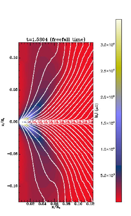
Figure 13: Structure of the azimuthally averaged magnetic field in the model having $\mu=2$ at time $t=1.5304\tau_{ff}$. The solid lines displays the poloidal magnetic field lines. They are overplotted on a snapshot of the toroidal magnetic field strength.

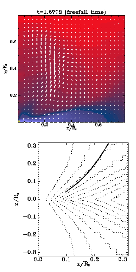
Figure 14: Upper panel: density and velocity field in the model having $\mu=2$ and a critical density $\rho_{c}/10$ at time $t=1.67\tau_{ff}$. Lower panel: structure of the azimuthally averaged poloidal magnetic field lines (dashed line) in the region of the outflow. The dashed lines show the global structure of those lines, while the thick line mark the selected magnetic field line along which some quantities will be plotted in Fig. 15. Note the different scale of the plot compared to Fig. 13.

Figure 15: First panel: angle $\theta$ (in degrees) between the poloidal fluid velocity and the poloidal magnetic field along the particular poloidal field line shown in figure 14. Note that $\theta$ is smaller than $10$ degrees, showing a good alignment between both vector. Second panel: Lorentz force (solid line) and pressure force (dashed line) exerted on the fluid element along the same magnetic field line. At all positions, the former exceeds the latter by one or two orders of magnitude, indicating that the outflow is largely magnetically driven. Third panel: Fluid velocity along the magnetic field line shown in Fig. 14. The gas is seen to be constantly accelerated because of the action of the Lorentz force (see fig. 15). It reaches a maximum outflow velocity of the order of $1.5$ km/s.

Figure 16: Angle between the poloidal magnetic field lines and the disk plane close to the disk surface. The analytical theory predicts that this angle should be larger than 30 degrees in the outflow launching region.

4.2.1 Basic features

In the case $\mu=2$, a collimated outflow developed quickly, as seen in Fig. 12. The first time displays the density and velocity fields just before the outflow is launched. The second time shows the early phase of the flow whereas the third time shows a more advanced phase after which the flow characteristics do not evolve much (see next section).

The morphology of the flow is quite different from what is obtained in the previous case. In particular, there is no slow magnetic tower as in the previous case. This is because, as discussed in Sect. 3, there is no centrifugally supported disk, instead a collapsing magnetic pseudo-disk forms. The outflows seem to emerge from the central thermally supported core with an angle of about $40-45$ degrees with respect to the z-axis and quickly recollimates. Figure 13 shows the structure of the magnetic field lines and strength of the toroidal magnetic field. The poloidal magnetic field is seen to be mostly vertical, particularly away from the equatorial plane. Close to the equatorial plane, the magnetic field lines are significantly inclined because of the inflowing fluid motions.

This is qualitatively in good agreement with the now classical model of the magneto-centrifugal ejection first described by Blandford & Payne (1982) and obtained in many simulations of magnetised disks (e.g. Pudritz et al. 2006). In the following section, a more quantitative analysis is presented.

4.2.2 Detailed analysis

The flow features described above tend to suggest that the outflows we found in this model are magneto–centrifugally driven. This type of outflow motion has been studied by many authors using self–similar techniques (Blandford & Payne 1982, Pelletier & Pudritz 1992) and assuming stationarity and axisymmetry. Therefore, in order to get the late phase evolution of the outflow for which it is expected that stationarity has been reached, we again use the model with a reduced critical density as its dynamical evolution is faster (larger timesteps in the thermally supported core), therefore allowing to get more easily the stationary regime. All figures were obtained after making an azimuthal average of the variables around the vertical axis.

The density and velocity fields are shown in the upper panel of Fig. 14. The flow is similar to that obtained with a critical density equal to $\rho_{c}$. To study quantitatively various outflows quantities, we focus on the parts of the outflow which are close to the equatorial plane ($z/R_{0}\leq 0.32$). Further away from the disk midplane, the outflow hits the inflowing material and its structure is perturbed. The poloidal magnetic field lines in this inner region are represented in Fig. 14 with dotted lines. The outflow properties are computed along one such field line, represented using the thick solid line in Fig. 14. One of the predictions of the theories mentioned above is that poloidal velocities $\bf{v_{p}}$ and magnetic field $\bf{B_{p}}$ are aligned when the outflow is in steady state. We plot in the upper panel of Fig. 15 the variation of the angle $\theta$ they make as one moves along that selected field line. Apart from the very inner part of the outflow ($z\leq 0.08$, which corresponds to the outflow launching region), $\theta$ is everywhere smaller than $10$ degrees, indicating a good alignment between the velocity and the magnetic field. In general, over the entire outflow region, we found that this angle is always smaller than $25$ degrees. This is a good indication that the outflow has come close to reaching steady state, which is in agreement with visual inspections of animations of this simulation. The middle panel of Fig. 15 gives an insight into the launching mechanism, by plotting the profile of the forces acting on the fluid along the same field line. The solid line shows the variation of the component of the Lorentz force along that field line. It is compared with the pressure gradient, also projected in the same direction. The former is clearly larger than the later, by one or two orders of magnitude: the outflow is magnetically (as opposed to thermally) driven. Finally, we also give the profile of the outflowing velocity along the magnetic field line (bottom plot of fig. 15). Because of the magnetic force, it increases steadily in the outflow to reach values of the order of $1.5$ km/s.

Another important prediction of the analytical self-similar model (Blandford & Payne 1982) is that the angle between the magnetic field lines close to the disk and the z-axis, should be larger than 30 degrees. In Fig. 16, we show this angle as a function of the radius. It has been measured at the disk surface, defined at each radius as being the altitude at which the radial fluid velocity vanishes. It is seen that this angle is indeed always larger than 30 degrees except in the very center and in the outer part. In these two regions, no outflow is occurring as can be seen in Fig. 14.

Figure 17: Ratio of ejection over accretion mass rate as a function of time. Upper panel is $\mu=20$ and lower panel $\mu=2$. Accretion and ejection mass rates are estimated on a sphere of radius $R_{s}$. Solid lines are for $R_{s}/R_{0}=0.2$, dotted lines for $R_{s}/R_{0}=0.4$ whereas dashed lines are for $R_{s}/R_{0}=0.6$.

Figure 18: Ratio of ejection over accretion angular momentum rate as a function of time. Upper panel is $\mu=20$ and lower panel $\mu=2$. Accretion and ejection angular momentum rates are estimated on a sphere of radius $R_{s}$. Solid lines are for $R_{s}/R_{0}=0.2$, dotted lines for $R_{s}/R_{0}=0.4$ whereas dashed lines are for $R_{s}/R_{0}=0.6$.

4.3 Mass and angular momentum fluxes

We now present quantities which characterize globally the evolution of the whole accretion-ejection structure with time. For this purpose we again use the simulations with the critical density, $\rho_{c}/10$, since they allow to follow the cloud evolution further.

Figures 17 and 18 display the ratio of ejected over accreted mass and angular momentum fluxes. They are estimated on spheres of various radius $R_{s}$, namely $R_{s}/R_{0}=0.2$ (solid lines), $R_{s}/R_{0}=0.4$ (dotted lines) and $R_{s}/R_{0}=0.6$ (dashed lines). Note that for $\mu=20$, the first value of $R_{s}$ is inside the magnetic tower whereas the 2 other values correspond to radius higher than the equatorial radius of the magnetic tower.

For $\mu=20$ and $R_{s}/R_{0}=0.2$, the ratio of ejection over accretion mass rate vanishes before $t=1.3\tau_{ff}$, then increases until a value of about 3-4. At this point quasi-stationarity is reached. This indicates that because of the centrifugal barrier, the gas first piles up in the inner region. Then the magnetic tower and the outflow described previously extract efficiently the mass at a rate higher than the accretion mass rate. For the two larger values of $R_{s}$, the ratio of ejection over accretion mass rate is smaller by a factor of about 3. This is due to higher accretion rates in the collapsing envelope than in the inner centrifugally supported structure.

The behaviour for $\mu=2$, is much different. The ratio of ejected over accreted mass rate varies between 0.1 and 0.6 and is therefore always smaller than 1. It increases with $R_{s}$. In that case, the gas falls directly in the centre without piling up in a centrifugally supported structure. The saturated ratios obtained for the two smallest $R_{s}$ are reminiscent of typical values quoted in the literature.

The ratio of ejection over accretion angular momentum rates have a similar behaviour than the ratio of ejection over accretion mass rates. However, we note that for $\mu=20$, the former is smaller than the later by a factor 1 to 2 whereas for $\mu=2$, the contrary is true (the ratio being as high as 3). These differences are due to the fact that in case $\mu=20$, the transportation of the angular momentum is weak since the magnetic tension is weak. Therefore the angular momentum is not transferred efficiently and is mostly advected with the gas. Since the gas which is accreted comes from larger radius than the gas which is ejected, the later has on average a larger angular momentum than the former. On the contrary, in case $\mu=2$, the gas is efficiently braked near the equatorial plane whereas it is azimuthally accelerated at higher altitude therefore carrying with it a higher angular momentum.

5 Comparison with observations

Here we qualitatively discuss comparisons between the models presented in the previous sections and various observations. One of the difficulties in carrying out detailed comparisons between observations and models of protostellar dense core is the need for sources sufficiently constrained observationally.

5.1 The case of IRAM04191

In this respect, the 1.5 solar mass, young class 0 source IRAM04191 (André et al. 1999, Belloche et al. 2002) located in the Taurus molecular cloud, is a nice example. In this elongated source, an outflow perpendicular to the major axis of the source has been observed suggesting that the rotation axis is also perpendicular to the major axis. With these assumptions, the rotation velocity has been measured. Moreover, the radial velocities and the column density profile are known as well from radiative modeling of the line profiles. A dynamical age of $\simeq$2 10⁴ years has been estimated from the characteristic of the flow. Finally, no disk has been detected in this source, the upper limit for the disk radius being around 15 AU.

Various attempts have been made to compare these profiles with hydrodynamical models, starting initially with critical Bonnor-Ebert sphere in rotation (Belloche 2002, Hennebelle et al. 2004b, Lesaffre et al. 2005). These models fail to reproduce IRAM04191 for the following reasons. First, the infall velocity ($\simeq$ 0.15 km/s) is too large at $r\simeq 2000$ AU in the model (0.2-0.3 km/s). Second the column density in the inner part ($r<1000$ AU) is too large in the model. In the model, the large column density in the inner region is due to the influence of rotation (see Fig. 1) which provides a support to the infalling gas. Self-consistently, the rotation curve cannot be reproduced under simple assumptions on the initial angular momentum distribution. In particular, the rotation velocity of the hydrodynamical model tends to be too high in the inner part. Another important related disagreement, is the absence of a big massive disk in IRAM04191 like the one produced in the hydrodynamical simulation.

Although no detailed comparison has been carried out, it seems worthwhile to compare with the magnetized models presented in this paper qualitatively. The first interesting aspect is the infall velocity which is smaller in the outer part than in the hydrodynamical case because of magnetic support. Although in the models presented here, it is still too large to reproduce the infall of IRAM04191, starting with near equilibrium configuration will help to reduce it further. However, running specific models dedicated to this particular case is beyond the scope of this paper. The second aspect is the rotation curve, which is much flatter in the $\mu=2-5$ cases than in the hydrodynamical case. This is also in better agreement with the rotation curve inferred for IRAM04191. Finally, the models with $\mu<5$ do not show the presence of hundred AU size disk unlike the hydrodynamical model. It is indeed, extremely difficult to reconcile the absence of disk and the presence of rotation within the framework of hydrodynamical models.

Another interesting aspect is the outflow which is observed in IRAM04191 (André et al. 1999). Its velocity is about 5-10 km/s. This is qualitatively in good agreement with the outflows spontaneously launched in the MHD models. Quantitatively, however, this is 2 to 5 times larger than the values obtained in this paper (note that outflow velocities up to $\simeq$3 km s^-1 are produced in our simulations). Nevertheless, as recalled previously, one should remember that the speed of the outflow is related to the rotation velocity achieved by the fluid particles. Since the physics of the first Larson core and the second collapse are not treated in this work, further contraction of the gas is prevented and therefore the velocity of the outflow is reduced. It seems therefore reasonable to assume that a better treatment of the first Larson core will yield to faster outflows (see Banerjee & Pudritz 2006, Machida et al. 2007).

5.2 Observations of class 0 sources with disk

While disks are commonly observed during the late stage of star formation, i.e. class I, class II or T Taury phase (e.g. Watson et al. 2007), disks are more difficult to observe during the class 0 phase and therefore much less constrained (Mundy et al. 2000). Nevertheless, various studies report class 0 protostars having disks of masses between 1 and 10 percents of their envelope masses (Looney et al. 2003, Jorgensen et al. 2007) giving a typical mass of about 0.1 solar mass.

Since the age of these sources is not well known and the density and velocity profiles are not available, it appears difficult to reach solid conclusions. This may nevertheless indicate that in these sources, the magnetic field is not too strong with typically $\mu>5$.

6 Conclusion

Using RAMSES, we performed 3D simulations of a magnetised collapsing dense core. We explored the effect of the initial magnetic field strength varying the value of the mass-to-flux over critical mass-to-flux ratio, $\mu$, from 1000 to 2. The cloud evolution is significantly modified for values as large as $\mu=20$. This is due to the strong amplification of the radial and azimuthal components of the magnetic field induced by the differential motions arising in the collapsing cloud.

We also developed semi-analytical models that predict some of the core envelope properties and compared them with the simulations results showing reasonable agreements.

For $\mu=20$, we find that magnetic braking is negligible and that consequently a centrifugally supported disk forms. A magnetic tower, generated by the twisting of the field lines, forms and expands reducing the mass of the centrifugally supported structures. A faster outflow is then triggered from the thermally supported central core.

For $\mu$ smaller than 5, no centrifugally supported disk forms for two reasons. First the collapse occurs primarily along the field lines which means that less angular momentum is delivered to the inner parts. Second, strong magnetic braking extracts the angular momentum from the disk. The question as to whether a disk will form at later stage remains nevertheless open. In addition, an outflow is triggered from the thermally supported core in that case. Detailed investigations have been performed in the case $\mu=2$. They reveal that the outflow reaches a quasi-steady state regime and features many characteristics of the magneto-centrifugally driven outflow models studied analytically in the literature (e.g. Blandford & Payne 1982, Pudritz et al. 2006).

In a companion paper, we study the fragmentation of the collapsing dense core paying particular attention to the strength of the magnetic field. The analysis developed in the present paper is then used to interpret the numerical results obtained in the context of fragmentation.

Appendix A An analytical model for the expansion of the magnetic tower with self-gravity

Figure 19: Density and transverse component of the magnetic field as given by Eqs. (29) and (30) for four times as a function of $z$.

We present an analytical model to investigate the mechanism responsible for the expansion of the self-gravitating disk.

In the simulation, the problem appears to be axisymmetric making it bidimentional. It is also evidently time dependent. For the purpose of reducing the complexity, we consider a self-gravitating layer which varies along the z-axis only, instead of an axisymmetric structure. We therefore replace, the azimuthal fields, $B_{\theta}$ and $V_{\theta}$ by the plane-parallel transverse fields $B_{x}(z)$ and $V_{x}(z)$. It is initially threaded by a vertical and uniform magnetic field, $B_{z}^{0}$. The transverse velocity, $V_{x}(z)$, initially generates a transverse magnetic field, $B_{x}(z)$ which modifies the vertical equilibrium. By doing so, we ignore the effect of the curvature inherent to the axisymmetric structure.

For simplicity, we make the approximation that the layer is in mechanical equilibrium and use Eq. (9) written previously. Let $\sigma=2\int\rho dz$ be the column density. With the Poisson equation, we get

$$\partial_{z}\psi=-2\pi G\sigma$$ (22)

Thus, defining

$$\widetilde{\rho}=\rho/\rho_{0}\,,\,\widetilde{\sigma}=\sigma/\sqrt{2\rho_{0}c_{s}^{2}/\pi G}\,,\,\widetilde{B}_{x}=B_{x}/B_{0},$$ (23)

where $B_{0}=\sqrt{4\pi\rho_{0}c_{s}^{2}}$, we get, since $\sigma(0)=0$ and $B_{x}(0)=0$,

$$\widetilde{\rho}+\widetilde{\sigma}^{2}+{\widetilde{B_{x}}^{2}\over 2}=1,$$ (24)

where $\rho_{0}$ is the density at $z=0$.

In order to compute $B_{x}$, we write the transverse momentum and induction equations using the Lagrangian coordinates (Shu 1983). With $\widetilde{t}=t/t_{0}$ where $t_{0}=1/\sqrt{2\pi\rho_{0}G}$, and $\widetilde{z}=z/z_{0}$ where $z_{0}=\sigma_{0}/2\rho_{0}$ we have

$$d_{\widetilde{t}}\widetilde{V}_{x}=\widetilde{B}_{z}^{0}\partial_{\widetilde{\sigma}}\widetilde{B}_{x},$$ (25)

and

$$d_{\widetilde{t}}\left({\widetilde{B}_{x}\over\widetilde{\rho}}\right)=\widetilde{B}_{z}^{0}\partial_{\widetilde{\sigma}}\widetilde{V}_{x}$$ (26)

This equation shows that, in the model, the growth of the toroidal field is triggered only by the vertical gradient of $V_{x}$, the transverse velocity. It is worth stressing that this equation does not include all the physical relevant terms in the problem. In particular, in the simulation the growth of the toroidal field is largely due to the twisting of the radial component of the magnetic field by the differential rotation which cannot be included in a plane parallel geometry. We note however that Fig. 11 clearly shows vertical gradients of $V_{\theta}$ ($z>10^{-4}$ pc at time 1.116 and 1.125 $\tau_{ff}$).

Equations (24), (25) and (26) are to be solved. Despite the simplifications, i.e. dependence on $z$ only and mechanical equilibrium in the vertical direction, they are still complex two variable non-linear equations. Since the disk is symmetric with respect to the equatorial plane, the boundary conditions are $B_{x}(0)=0$ and $\partial_{\sigma}V_{x}(0)=0$.

In order to illustrate the origin of the expansion due to the growth of the toroidal magnetic component, we consider as initial conditions a self-gravitating layer with a vanishing $B_{x}$ at time $\widetilde{t}=0$. In that case the solution is simply $\widetilde{\rho}=1-\widetilde{\sigma}^{2}$. In term of the $\widetilde{z}$ variable, this writes $\widetilde{\rho}(\widetilde{z})=1/{\rm ch}(2\widetilde{z})^{2}$ (Spitzer 1942, Ledoux 1951, Curry 2000).

Since obtaining exact solutions of Eqs. (24)-(26) seems to be difficult, we seek approximated solutions of the equations written above. To this purpose, we replace Eq. (26) by

$$d_{\widetilde{t}}\widetilde{B}_{x}=\left(1-\widetilde{\sigma}^{2}\right)\partial_{\widetilde{\sigma}}\widetilde{V}_{x},$$ (27)

that is to say, we assume that the density in Eq. (26), is the density of the unmagnetised solution. Strictly speaking, this approximation holds as long as the density has not been modified by the magnetic field significantly. With this assumption, the time and space variables separate, making it easy to find solutions as

$$\widetilde{V}_{x}(\widetilde{t},\widetilde{\sigma})=\widetilde{V}_{0}\cos(\sqrt{6}B_{z}^{0}\widetilde{t})\times(1-3\widetilde{\sigma}^{2}),$$ (28)

$$\widetilde{B}_{x}(\widetilde{t},\widetilde{\sigma})=-\sqrt{6}\widetilde{V}_{0}\sin(\sqrt{6}\widetilde{B}_{z}^{0}\widetilde{t})\times(\widetilde{\sigma}-\widetilde{\sigma}^{3}).$$ (29)

Using Eq. (24), we obtain the density as a function of $\widetilde{\sigma}$ and $\widetilde{t}$

$$\widetilde{\rho}=1-\widetilde{\sigma}^{2}-3\widetilde{V_{0}}^{2}\sin^{2}(\sqrt{6}\widetilde{B}_{z}^{0}\widetilde{t})(\widetilde{\sigma}-\widetilde{\sigma}^{3})^{2}.$$ (30)

using the relation $d\sigma=2\rho dz$, it is possible to obtain $z$ as a function of $\sigma$ and $\rho$.

Figure 19 shows $\widetilde{\rho}$ and $\widetilde{B}_{x}$ as given by Eqs. (29) and (30) at four times for $\widetilde{V}_{0}=2$ and $\widetilde{B}_{z}^{0}=1$. The behaviour is very similar to the evolution displayed in Fig. 11. As $\widetilde{B}_{x}$ is growing, the layer is expanding because of the magnetic pressure.