Local and Nonlocal Dispersive Turbulence

Abstract

We consider the evolution of a family of two-dimensional (2D) dispersive turbulence models. The members of this family involve the nonlinear advection of a dynamically active scalar field, and as per convention, the locality of the streamfunction-scalar relation is denoted by $\alpha$, with smaller $\alpha$ implying increased locality ($\alpha=1$ gives traditional 2D dynamics). The dispersive nature arises via a linear term whose strength, after non-dimensionalization, is characterized by a parameter $\epsilon$. Setting $0<\epsilon\leq 1$, we investigate the interplay of advection and dispersion for differing degrees of locality. Specifically, we study the forward (inverse) transfer of enstrophy (energy) under large-scale (small-scale) random forcing along with the geometry of the scalar field. Straightforward arguments suggest that for small $\alpha$ the scalar field should consist of progressively larger isotropic eddies, while for large $\alpha$ the scalar field is expected to have a filamentary structure resulting from a stretch and fold mechanism; much like that of a small-scale passive field when advected by a large-scale smooth flow. Confirming this, we proceed to forced/dissipative dispersive numerical experiments under weakly non-local to local conditions (i.e. $\alpha\leq 1$). In all cases we see the establishment of well-defined spectral scaling regimes. For $\epsilon\sim 1$, there is quantitative agreement between non-dispersive estimates and observed slopes in the inverse energy transfer regime. On the other hand, forward enstrophy transfer regime always yields slopes that are significantly steeper than the corresponding non-dispersive estimate. At present resolution, additional simulations show the scaling in the inverse regime to be sensitive to the strength of the dispersive term : specifically, as $\epsilon$ decreases, quite expectedly the inertial-range shortens but we also observe that the slope of the power-law decreases. On the other hand, for the same range of $\epsilon$ values, the forward regime scaling is observed to be fairly universal.

I Introduction

It is quite common in geophysical fluid dynamics to encounter problems that involve the presence of both advection and dispersion (see for example, Chapter 5 in the text by Majda Majda-book and Chapter 5 in the text by Chemin et al. Chemin-book ). In a two-dimensional (2D) context, simple model equations that possess advection and dispersion include the familiar barotropic beta plane equations Rhines and the dispersive surface quasigeostrophic (SQG) equations HPGS . An interesting aspect of such equations, highlighted by Rhines Rhines in the barotropic beta plane case, is the co-existence of turbulent and wave-like motions HH , Shep . In fact, the dispersive SQG equations have been proposed as an alternate (more local) platform for investigating wave-turbulence interactions HPGS .

In the present work, we look at an extended family (that includes the aforementioned examples as members) of dispersive active scalars. This is a simple dispersive generalization of the family of 2D turbulence models introduced in Pierrehumbert, Held & Swanson PHS . Specifically, in a 2D periodic setting we consider

$$\frac{D\theta}{Dt}+\frac{1}{\epsilon}\frac{\partial\psi}{\partial x}=0~{};~{}(u,v)=(-\frac{\partial\psi}{\partial y},\frac{\partial\psi}{\partial x})$$

$$~{}\textrm{where}~{}~{}\hat{\theta}(k_{x},k_{y},t)=-(k^{2})^{\alpha}\hat{\psi}(k_{x},k_{y},t)$$ (1)

where $D/Dt$ denotes the 2D material derivative and $\epsilon$ is a non-dimensional parameter. Note that in real space $\theta$ and $\psi$ above are related via a suitable (pseudo-) differential operator, i.e. $\theta=-(-\triangle)^{\alpha}\psi$ where $\triangle$ is the 2D Laplacian, and for our purposes $\alpha\in\Re^{+}$. For the beta plane equations we have $\alpha=1$, $\theta$ is the vorticity field, and $\epsilon$ corresponds to the Rhines number $Rh=U/(\beta L^{2})$. In the dispersive SQG case $\alpha=1/2$, $\theta$ represents the buoyancy (or potential temperature HPGS ), and $\epsilon=U/(\Lambda L)$. Physically, of course we are dealing with very different scenarios wherein $\beta$ is the ambient planetary gradient of the vorticity while $\Lambda$ is the background surface buoyancy gradient. Apart from $\alpha=1,1/2$, there exist other members of this family that have physical interpretations Smithetal . But, from a broader perspective, the entire family is well defined, and we expect that varying $\alpha$ would provide greater insight into the interplay between advection and dispersion.

We begin examining the effect of $\alpha$ on the dynamics by suppressing the dispersive term. After developing a feel for the dependence of the energy/enstrophy transfer and the geometry of the scalar field on $\alpha$, we introduce dispersion and note its modulating effect on the nonlinear term. In the limit $\epsilon\rightarrow 0$, the so-called limiting dynamics are controlled by resonant interactions. In fact, the resonant skeleton corresponding to (1) is seen to be of the same form as that of the rotating three-dimensional (3D) Euler equations. Following the original argument by Rhines Rhines , for $0<\epsilon\leq 1$, if $\alpha>0.5$, the simultaneous transfer of energy to large scales and small frequencies leads to an anisotropic streamfunction (resulting in predominantly zonal flow). In contrast, given the nature of the dispersion relation, it turns out that for $\alpha<0.5$ the constraints of energy transfer to large scales and small frequencies do not require the spontaneous development of anisotropy in the streamfunction. Confirming this via decaying runs from spatially un-correlated initial data, we proceed to a suite of forced/dissipative numerical simulations. In all cases, under weakly-local to local conditions (i.e. $\alpha\leq 1$) we note the formation of clear power-law scaling. The various slopes are extracted and compared with non-dispersive estimates. The paper ends with a collection of results and a brief discussion of potentially interesting avenues for future work.

II Some observations on the effect of $\alpha$

Before considering the effect of dispersion, we examine the influence of $\alpha$ in greater detail. To get a feel for the locality of the interactions, we shut off the linear dispersive term in (1) and consider a simple numerical exercise involving the evolution of a smooth $\theta$ ring. As is seen in Fig. (1), the deformation of the ring is more physically local for smaller $\alpha$. Given that $\hat{\psi}(\vec{k})=-\hat{\theta}(\vec{k})/k^{2\alpha}$, as $\alpha$ increases, one sees that only the small $k$ features of $\theta$ and $\psi$ remain dynamically active. As a result, for larger $\alpha$, smaller scale features of the scalar field are for all purposes driven in a passive manner. In fact, in the limit $\alpha\rightarrow\infty$, only the wavenumber one ($k=1$) component of $\theta$ and $\psi$ is coupled, and we end up with the problem of passive advection via a large-scale smooth flow. In contrast, the case of small $\alpha$ is markedly different. Specifically, $(\hat{u},\hat{v})=({\rm i}k_{y}\hat{\theta}/k^{2\alpha},-{\rm i}k_{x}\hat{\theta}/k^{2\alpha})$ results in a transition at $\alpha=1/2$ (when the scalar and velocity fields have similar scales), where for $\alpha<1/2$, the velocity fields are in fact of a finer scale than the advected scalar field. Note that $\psi$ remains a smoothened form of $\theta$. We expect this transition to have interesting consequences as there are well-known differences in the behavior of a passive field when advected by large-scale, comparable-scale and small-scale flows respectively SP ,FH ,MajdaKramer .

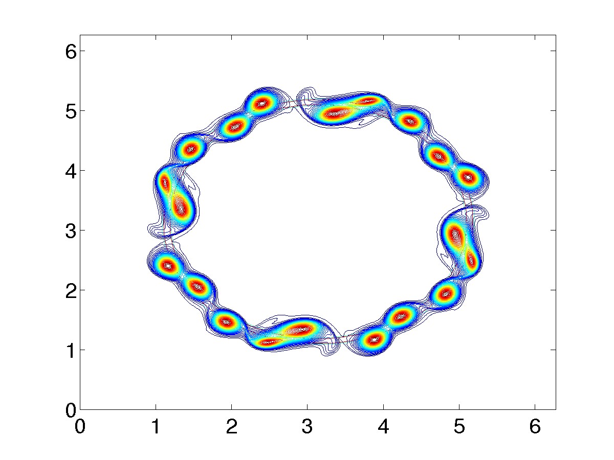
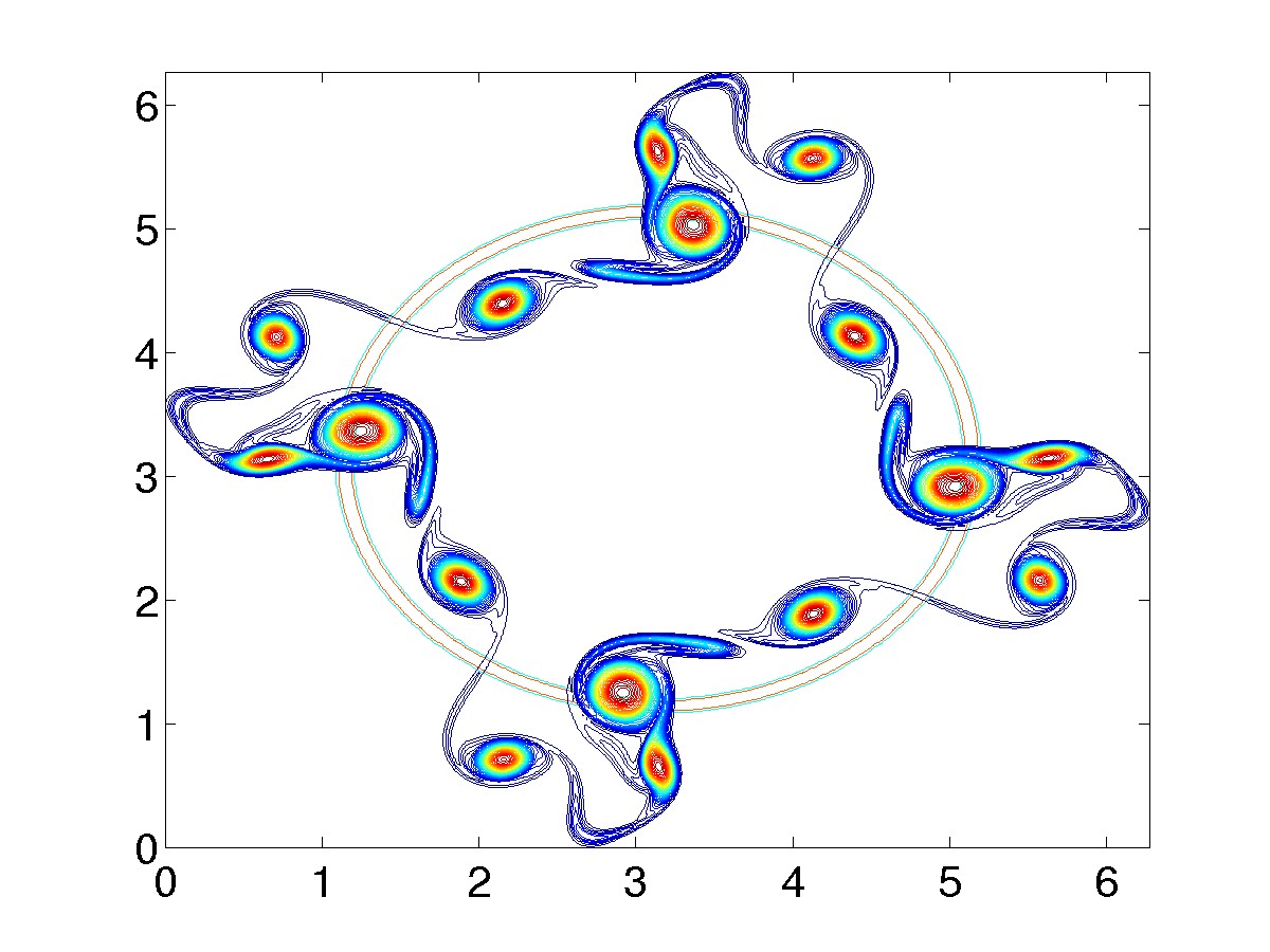
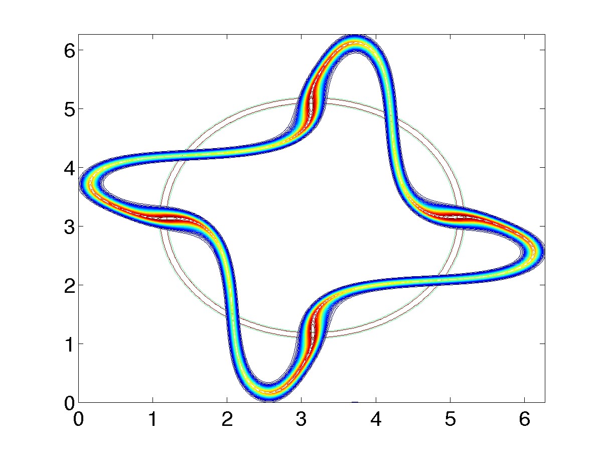
Figure 1: Non-dispersive evolution of $\theta$ rings. From left to right, $\alpha=0.5,1$ and 1.5 respectively. Quite clearly, for smaller $\alpha$ the deformation is more local in character.

In a 2D periodic domain, much like its non-dispersive counterpart, (1) conserves energy $E=\int_{\bf D}\psi\theta$ and enstrophy or ”$\theta$-variance” ${\mathcal{E}}=\int_{\bf D}\theta^{2}$. Continuing with the non-dispersive case, following arguments for the 2D Euler equations Kraichnan1967 , it is expected that the energy primarily flows to large scales while the $\theta$-variance is transferred to small scales. Assuming the presence of an equilibrium cascade, detailed spectral scaling laws in the appropriate inertial-range have also been derived PHS , Smithetal , Watanabe (see also Tran Tran1 and Tran & Bowman Tran2 for bounds on the scaling exponents for certain special dissipative operators in the SQG case). If we consider the Fjortoft estimate (Fjortoft , Chapter 4 in Salmon Salmon-book ) i.e. the transfer of energy out of scale $k_{1}$ into scales $k_{0},k_{2}$ (s.t. $k_{0}=k_{1}/2a$ and $k_{2}=2ak_{1}$, where $a>1$), we have $E_{0}=E_{1}\times\{a^{2\alpha}/[1+a^{2\alpha}]\}$; i.e. the more nonlocal the situation ($\alpha>0.5$), the larger is the fraction of the energy (enstrophy) transferred to large (small) scales. Note that increasing $a$ shows this unequal distribution of energy and enstrophy is further exaggerated when the exchange involves scales that are progressively further apart, i.e. the energy/enstrophy partition is more biased in spectrally nonlocal transfers.

To develop a feel for the dependence of the geometry of an emergent scalar field on $\alpha$, we continue with non-dispersive simulations, though now from spatially un-correlated initial data chosen from a Gaussian distribution with unit variance. Given the presence of an inverse transfer of energy, we expect coherent structures to emerge from this un-correlated initial condition. In fact, given the similar scales of the velocity and scalar fields for smaller $\alpha$ we do not expect the scalar field to undergo much stretching and folding, while for large $\alpha$ we expect repeated events of this sort leading to a filamentary scalar field — much like the fate of a small-scale passive blob when advected by a large-scale smooth flow — due to the implicit large-scale strain (via the large scale-separation between $\theta$ and $\psi$). These expectations are confirmed in Fig. (2) which shows the initial condition and the emergent scalar field for $\alpha=0.5$ and $2$ respectively.

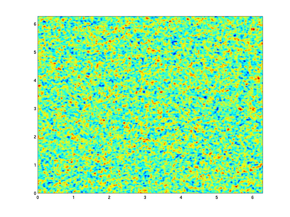
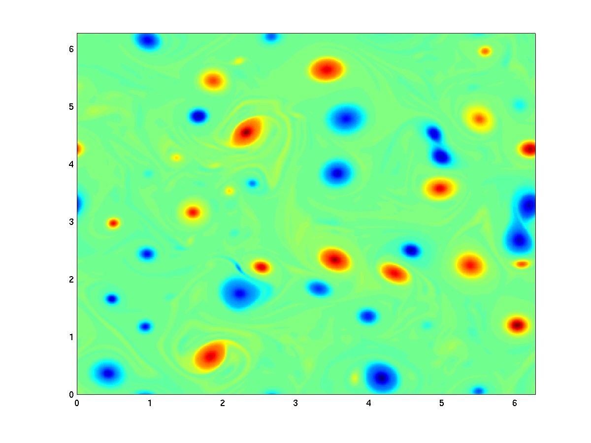
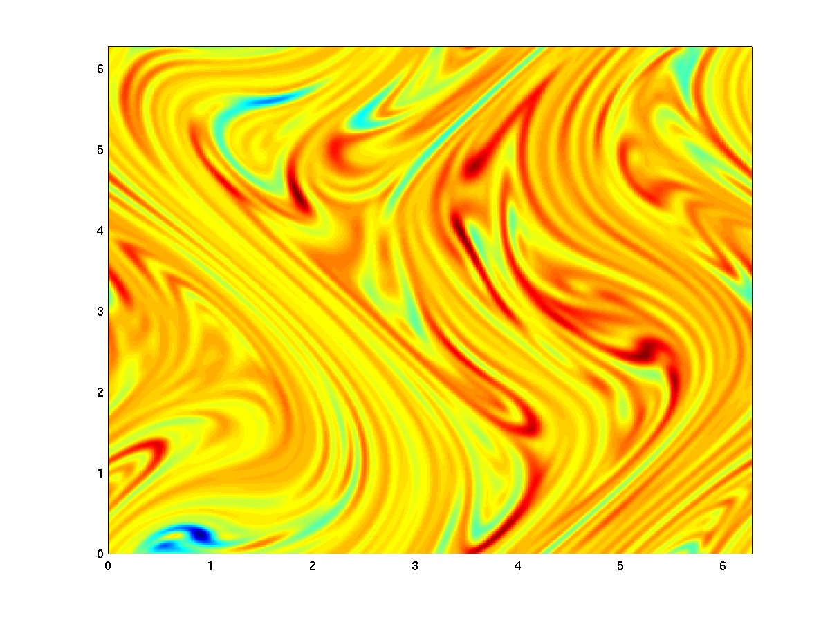
Figure 2: The first panel is the spatially un-correlated initial condition (smoothened via a diffusive stencil). The second and third panels show the emergent scalar field for $\alpha=0.5$ and $2$ respectively. Quite clearly, for $\alpha=0.5$ we have a field composed of coherent $\theta$ eddies while for $\alpha=2$ we obtain a filamentary geometry reminiscent of a passive field when subjected to large-scale advection.

III The influence of the dispersive term

When the dispersive term is included, the linearized form of (1) supports waves with the dispersion relation

$$\omega(\vec{k})=-\frac{k_{x}}{\epsilon k^{2\alpha}}~{}~{};~{}~{}\textrm{where}~{}~{}\vec{k}=(k_{x},k_{y})$$ (2)

It is interesting to note that, for $\alpha=0.5$, (2) gives $0\leq|\omega(\vec{k})|\leq 1/\epsilon$. For $\alpha<0.5,|\omega|\rightarrow\infty$ for $k_{y}=0,k_{x}\rightarrow\infty$, whereas for $\alpha>0.5,|\omega|\rightarrow\infty$ for $k_{y}=0,k_{x}\rightarrow 0$. The dispersion relation for different $\alpha$ (on either side of $\alpha=0.5$) is plotted Fig. (3). Quite clearly the frequencies have a very different dependence on wavenumber when $\alpha<,=$ or $>0.5$. In fact, an important feature of the beta plane equations (which is true for all $\alpha>0.5$) that $|\omega(\vec{k})|$ increases for large scales is no longer true for $\alpha\leq 0.5$; in fact, for $\alpha<0.5$ the smaller scale features have larger frequencies.

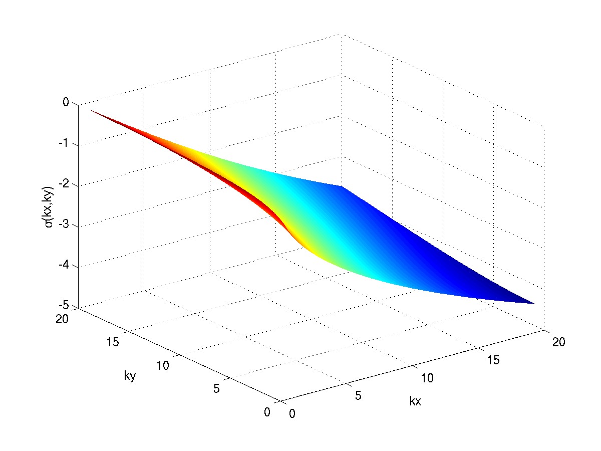
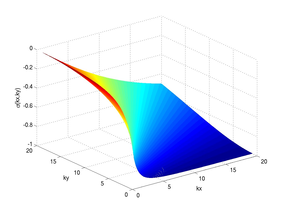
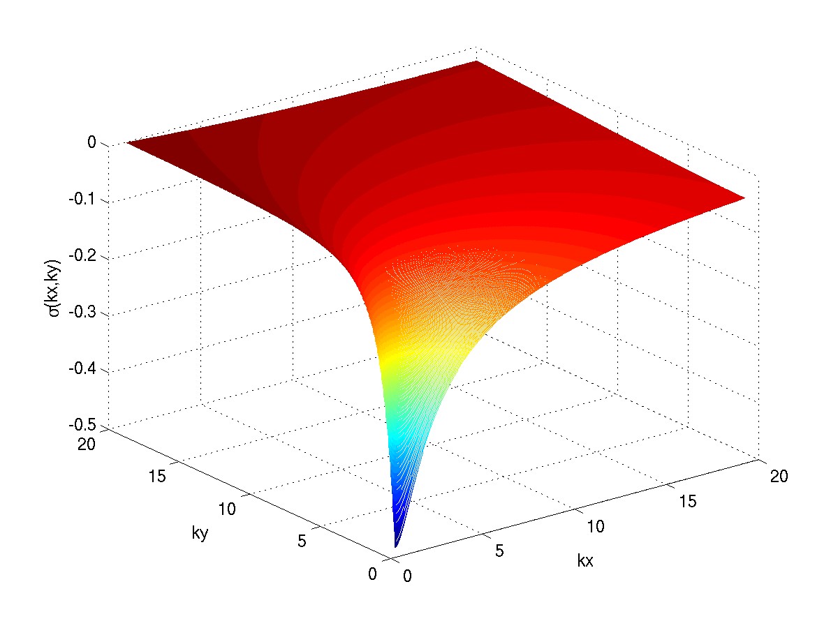
Figure 3: The dispersion relation (2) with $\epsilon=1$ for, from left to right, $\alpha=0.25,0.5$ and 1 respectively. Note that for $\alpha=0.5$ the frequencies are bounded while on either side we obtain $|\omega|\rightarrow\infty$ in particular limits.

In the following, we occasionally refer to modes with zero frequency as slow modes and those for which $\omega\neq 0$ as fast modes. In a periodic setting, substituting a Fourier representation in (1) yields

$$\frac{\partial\hat{\psi}_{k}}{\partial t}=\sum_{\mathcal{T}}C_{kpq}~{}\hat{\psi}_{q}\hat{\psi}_{p}~{}\exp\{\frac{-{\rm i}}{\epsilon}[-\frac{p_{x}}{p^{2\alpha}}-\frac{q_{x}}{q^{2\alpha}}+\frac{k_{x}}{k^{2\alpha}}]{\rm t}\}$$ (3)

where $\sum_{\mathcal{T}}$ represents a sum over $\vec{p},\vec{q}$ such that $\vec{k}=\vec{p}+\vec{q}$ and $C_{kpq}$ is the interaction coefficient given by

$$C_{kpq}=(p_{x}q_{y}-p_{y}q_{x})[\frac{p^{2\alpha}-q^{2\alpha}}{k^{2\alpha}}]$$ (4)

III.1 Zonal flows

Considering an initial value problem, the original deduction of anisotropic fields by Rhines Rhines , in the context of the beta plane equations was based on the dual constraint of an upscale transfer of energy along with the tendency of resonant triads to move energy into small frequencies (see Hasselmann Hass for a general demonstration irrespective of the details of the nonlinear coupling co-efficient). Indeed, the two pieces of the Rhines argument are : (i) energy moving to large scales as a result energy/enstrophy conservation, and (ii) the importance of resonant triads in energy transfer when dispersion modulates the advective nonlinearity. In the context of the general dispersion relation (2), for isotropic structures, $k_{x}\sim k_{y}\sim k$ we have

$$|\omega|=\frac{1}{\epsilon 2^{\alpha}}~{}\frac{1}{k^{2\alpha-1}}.$$ (5)

Hence for $\alpha>0.5$, moving to large scales, i.e. for decreasing $k$ we encounter larger frequencies. Therefore, to satisfy the dual constraints, Rhines Rhines suggested that the system would spontaneously generate anisotropic structures; further examining (2) shows that these constraints are satisfied for $k_{y}\neq 0,k_{x}/k_{y}\ll 1$. Also, when considering energy transfer into large scales, i.e. $k<p,q$, interactions that fall in the aforementioned anisotropic category are in fact near-resonant Salmon . In essence we have an anisotropic streamfunction that results in predominantly zonal flows. Though note that for $\alpha<0.5$, decreasing $k$ implies smaller frequencies, therefore it is possible to maintain isotropy while simultaneously transferring energy to large scales and small frequencies. Hence, for $\alpha<0.5$, the dual constraints do not nessecitate the formation of a dominant of zonal flow. Note that this does not imply zonal flows cannot form for $\alpha<0.5$, in fact, substituting an expansion of the form $\psi=\psi^{0}+\epsilon\psi^{1}...$, the $O(1/\epsilon)$ balance in (1) yields $\partial\psi^{0}/\partial x=0\Rightarrow u^{0}=u^{0}(y,t),v^{0}=0$. Of course, this expansion doesn’t imply any control over the higher order terms, but irrespective of $\alpha$, at order zero, it indicates the possibility of zonal flow formation.

A different, though complementary, approach to the generation of zonal flows is to view (1) as a mixing problem, i.e. to consider the mixing of $\theta$ in the presence of a background gradient Rhines-Young . In the context of the beta plane equations, as shown by Rhines & Young Rhines-Young , steady flows with closed streamlines (or gyres) result in the homogenization of potential vorticity between these streamlines. With a linear background, this naturally leads to a ”saw-tooth” vorticity profile with high gradients concentrated on the streamlines McDrit . Further in a statistically steady state, this reasoning posits the existence of successive ”saw-tooth” structures in the vorticity profile (or in other words a potential vorticity ”staircase”) if the size of the eddies is smaller than the size of the domain McDrit (see Danilov1 , Danilov2 for forced- dissipative simulations and Marcus-Lee for experimental results in this regard). From this viewpoint localized zonal flows (jets) result from an inversion of the aforementioned potential vorticity ”staircase”. For the general family in (1), $\theta+y/\epsilon$ is mixed by the flow and a similar homogenization within streamlines is expected to follow. Further, as the scale of the velocity field becomes smaller than that of the advected scalar when $\alpha$ crosses $0.5$ from above, we expect the homogenization for small $\alpha$ to progress in a more diffusive manner, i.e. small-scale inhomogeneties will be erased earlier which supports a gradual explusion of scalar gradients from small to large scales. In this vein, Fig. (4), much like the classic picture by McIntyre, reproduced in Dritschel & McIntyre McDrit , shows the inversion of a single ”saw-tooth” using the general form in (1). As is evident — apart from the known asymmetry in the east-west jets in the beta plane equations — the more local the inversion (i.e. for smaller $\alpha$) the narrower and stronger are the corresponding jets.

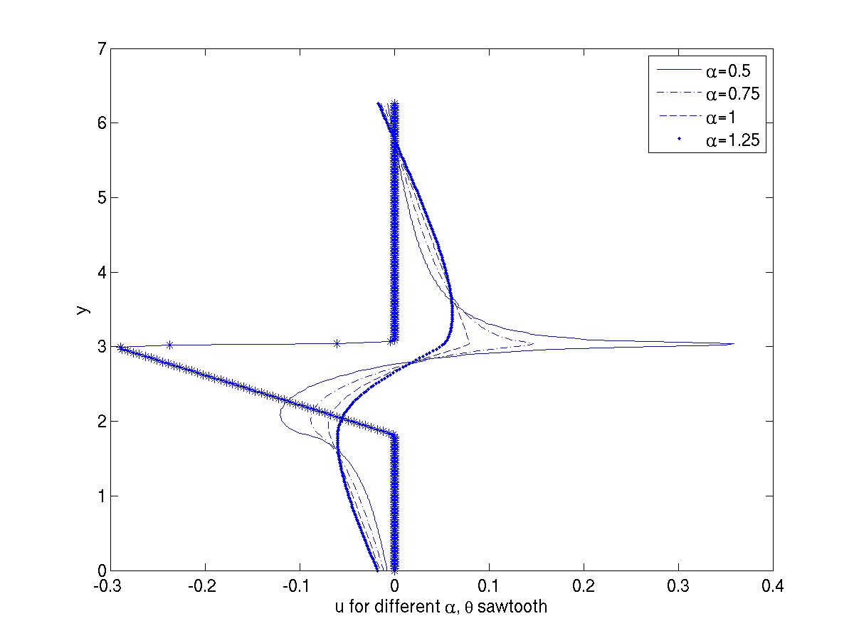
Figure 4: Inversion of a single ”saw-tooth” $\theta$ profile for varying $\alpha$. As is evident, in addition to the east-west asymmetry, smaller $\alpha$ (more local) gives stronger and narrower jets.

To examine the nature of emergent flows for differing locality in the presence of dispersion, we perform numerical simulations with spatially un-correlated initial data as shown in the first panel of Fig. (2). Setting $\epsilon=0.1$, the scalar and zonal component of the velocity fields for $\alpha=0.25,1$ and $\alpha=1.25$ are shown in Fig. (5), quite clearly for $\alpha>0.5$ we have, what might be termed a coherent zonal flow. Note that, in accord with Fig. (4), the flows are broader and of smaller magnitude for increasing $\alpha$.

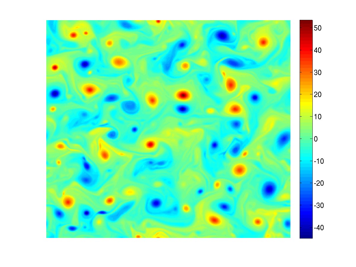
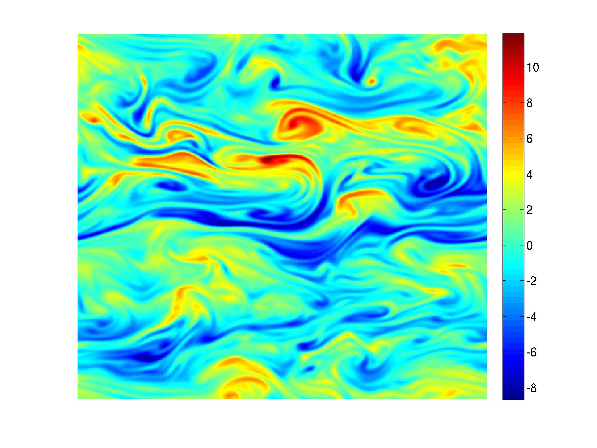
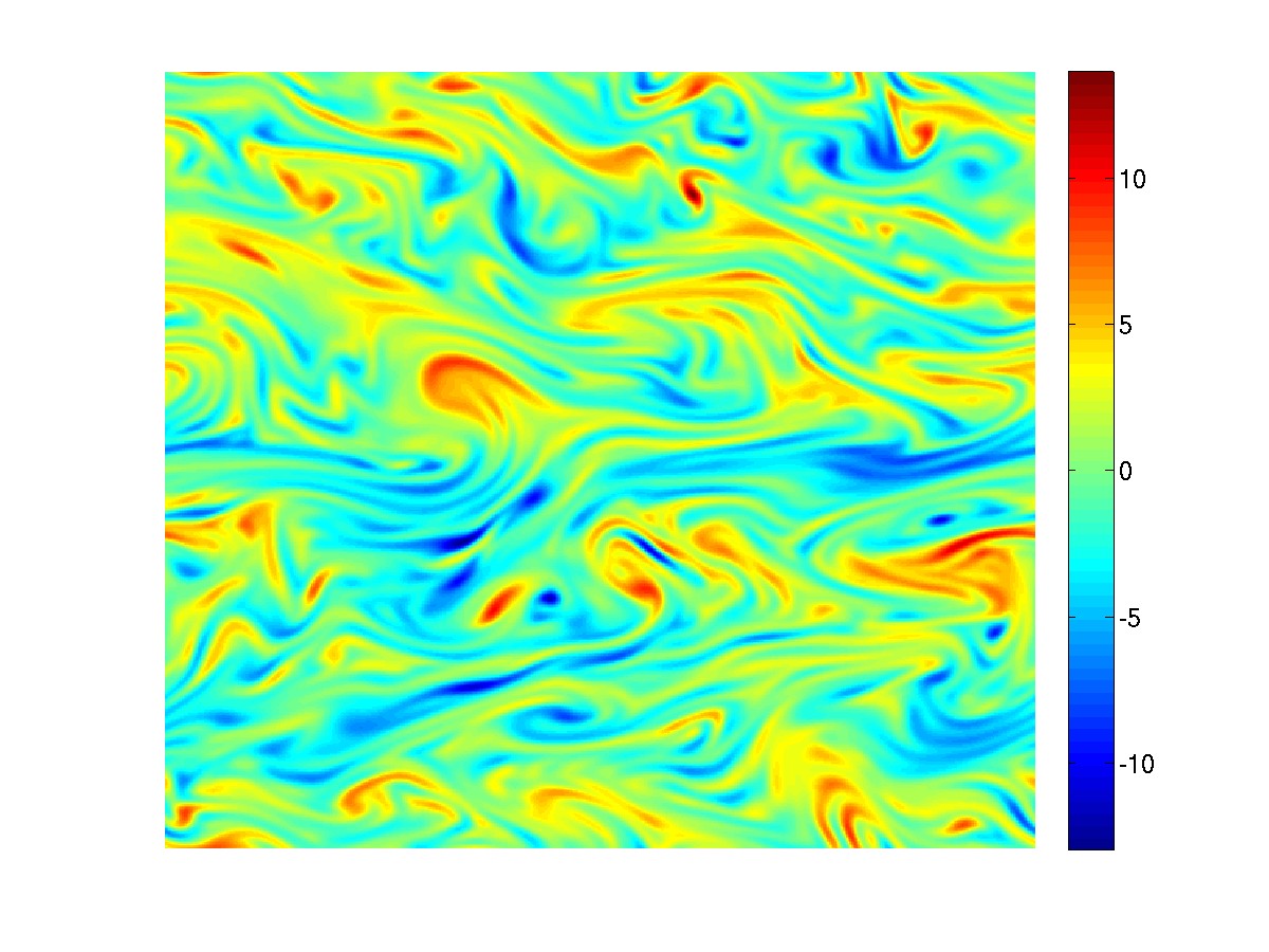
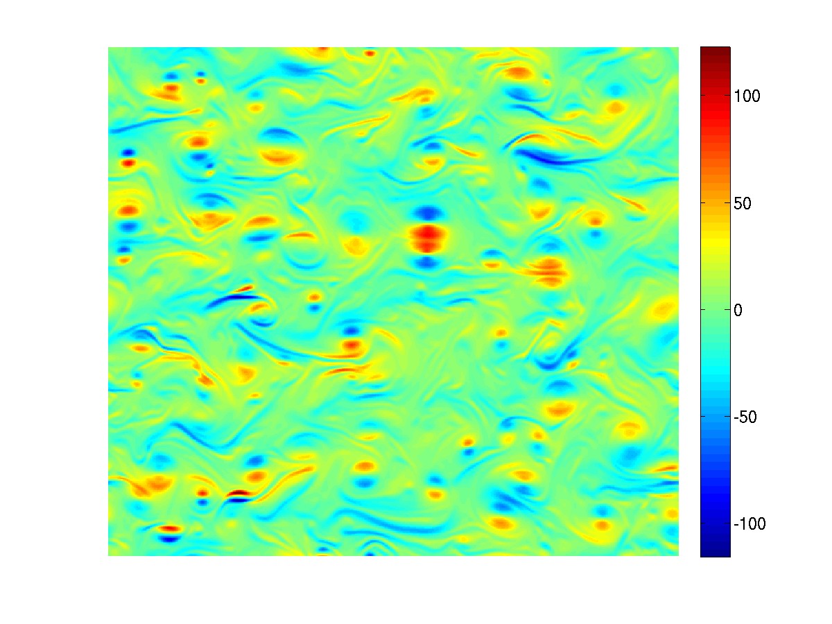
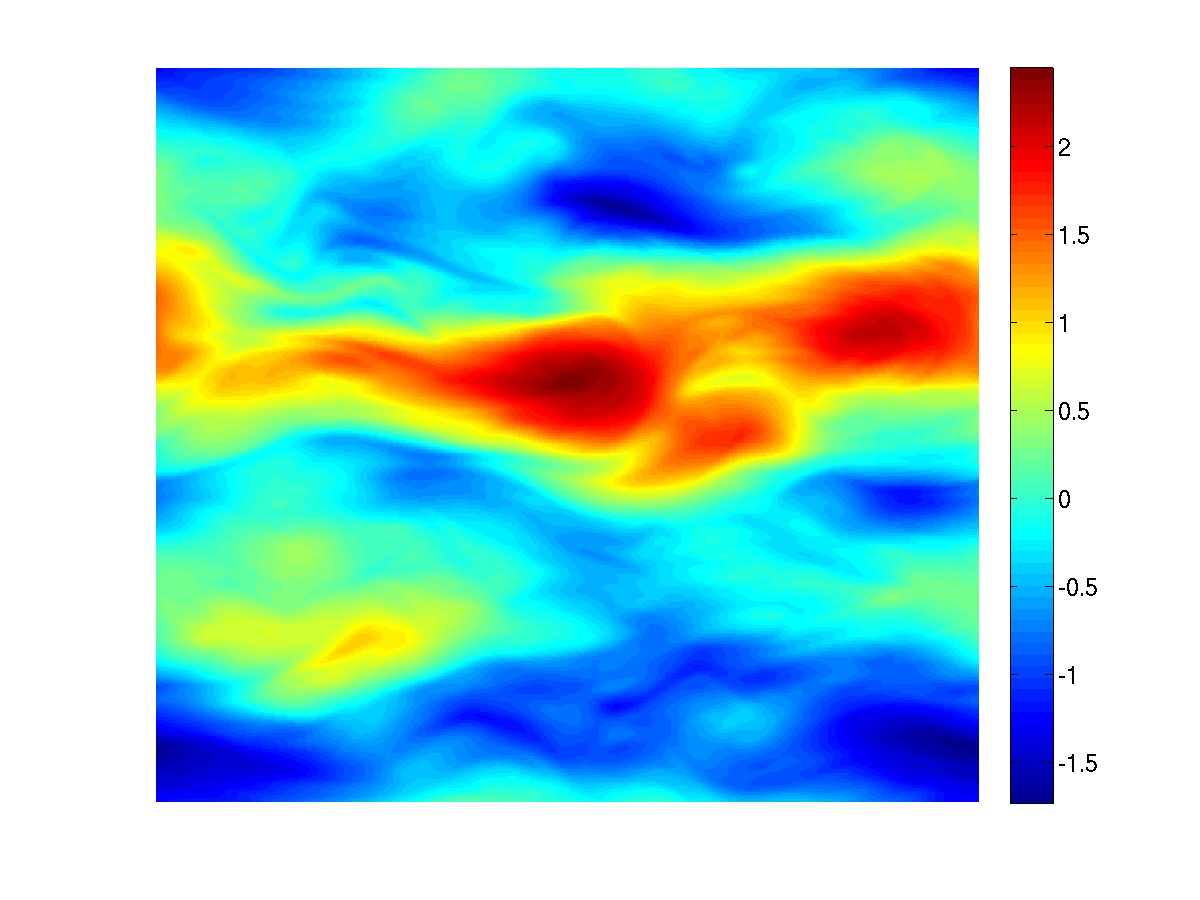
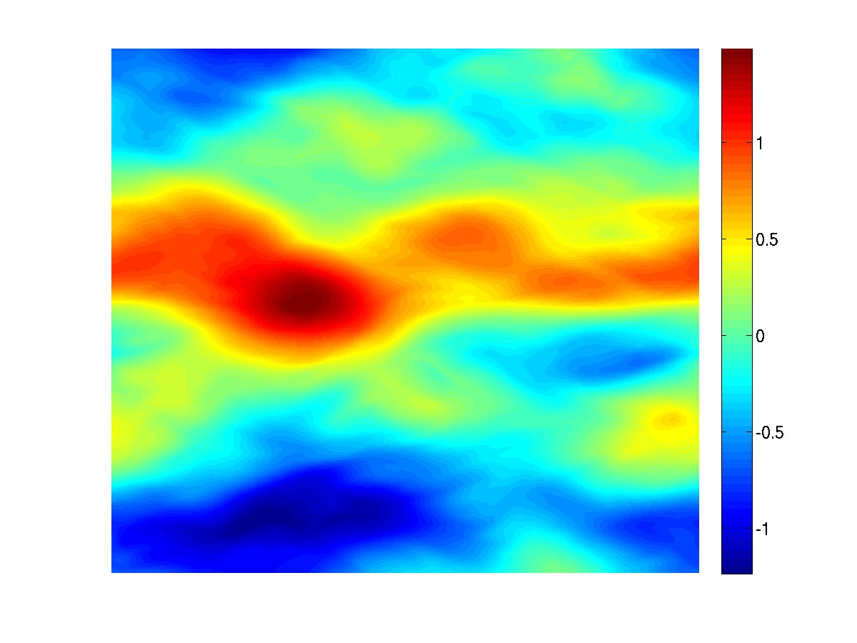
Figure 5: $\theta,u$ fields for $\alpha=0.25,1$ and 1.25 in the upper and lower panels respectively. In all cases $\epsilon=0.1$. Note the finer scale of the flow as compared to the scalar field when $\alpha=0.25$. Further for increasing $\alpha$, we obtain coherent zonal flows.

III.2 Resonant and near resonant interactions

Evolving (3) in time, in the limit $\epsilon\rightarrow 0$, given the highly oscillatory nature of the integrals involved, the only terms that contribute to (3) are those which are exactly resonant. Following the notation of Chen et al. Chen-etal , i.e. the first entry in a triplet $(\cdot,\cdot,\cdot)$ evolves via the interaction of the latter two entries, the limiting ($\epsilon\rightarrow 0$) dynamics are made up of :

• $p_{x}=q_{x}=k_{x}=0$ i.e. the slow-slow-slow ($s,s,s$) interactions : All such interactions between purely zonal flows are clearly resonant. However, from (4) we see that their interaction coefficients are zero.

• $k_{x}=0$, $p_{x},q_{x}\neq 0$ i.e. slow-fast-fast $(s,f,f)$ or fast-slow-fast $(f,s,f)$ interactions : It is easy to check that two modes with $\omega\neq 0$ cannot feed (extract) energy to (from) one with $\omega=0$. In other words, two fast modes cannot generate a zonal flow. On the other hand, two fast modes can interact with each other using a zonal mode as a catalyst and this represents the passive advection of the fast modes via a zonal shear flow.

• $k_{x},p_{x},q_{x}\neq 0$ i.e. the fast-fast-fast $(f,f,f)$ interactions : These are the three-fast wave interactions. Though they are algebraically difficult to achieve, these interactions represent fully 2D motion.

As is evident, this situation is entirely analogous to the analysis of the beta plane equations as presented by Longuet-Higgins & Gill LG . Further, there is a close correspondence between these resonant interactions and the limiting dynamics (i.e. when the Rossby number $\rightarrow 0$) of rotating three-dimensional (3D) flows. For the 3D rotating case Babin-rot1 , the analogous set of $(s,s,s)$ interactions result in purely 2D flow (though now with a non-zero interaction coefficient); the second set of $(f,s,f)$ interactions leads to the passive advection of the vertical velocity via this 2D flow and inclusion of the third set of $(f,f,f)$ resonances yields the so-called $2\frac{1}{2}$ dimensional equations. Further, transfer from exclusively fast to slow modes in pure rotation is also precluded under resonance, i.e. $(s,f,f)$ interaction has a zero interaction coefficient, where the zero frequency mode corresponds to a columnar structure. Therefore, in the limit $\epsilon\rightarrow 0$ (Rossby number $\rightarrow 0$), it is not possible generate a zonal flow (columnar structure) from exclusively non-zonal (non-columnar) initial data and forcing.

Of course, the limit $\epsilon\rightarrow 0$ is usually not of great physical interest, in fact we are usually more concerned with situations wherein $0<\epsilon\leq 1$. This opens the door to non-resonant interactions, and quite naturally, we expect near-resonances — i.e. triads for which $\omega(\vec{p})+\omega(\vec{q})-\omega(\vec{k})=\delta\ll\epsilon$ — to be of greater significance than the remainder that are, in terms of ($\delta,\epsilon)$, far from resonance. As the $(s,f,f)$ non-resonant triads have a non-zero interaction co-efficient we have the possibility of directly transferring energy from non-zonal to zonal modes. Choosing $\delta$ for given $\epsilon$, such transfer to slow modes has been numerically verified in the beta plane and 3D rotating systems Smith-qg , Smith-rot .

IV The inverse and forward cascades

With the aim of examining a systematic transfer of energy/enstrophy from one scale to another, we proceed to numerical simulations from weakly non-local to local conditions (i.e. $\alpha\leq 1$) Kraichnan1967 , Chen-2D . The numerical scheme is a de-aliased psuedospectral method with fourth order Runge-Kutta time stepping. All simulations are performed in Matlab at a resolution of $750\times 750$. Further, we supplement the RHS of (1) with hyper-viscous dissipation of the form $(-1)^{n+1}\nu_{n}\triangle^{n}\theta$ (to act as a sink at small scales, with $n=4$). As per Maltrud & Vallis Maltrud-Vallis we choose $\nu_{n}=\theta_{\textrm{rms}}/({k_{m}}^{2n-2})$, where $k_{m}$ is the maximum resolved wavenumber.

Denoting the domain, forcing and dissipation scales by $k_{L},k_{f}$ and $k_{d}$ respectively, we consider $k_{L}\ll k_{f}<k_{d}$ ($k_{L}<k_{f}\ll k_{d}$) which allows us achieve, for a given resolution, as large an inverse (forward) energy (enstrophy) transfer regime as is possible. The forcing is of random phase at every time-step and de-correlates with a time-scale $\tau$ (this is chosen to be comparable to the fastest linear wave in the model). Further the forcing is localized to a few wavenumbers, and it is important to note — especially in the context of a small-scale case — that our forcing is not chosen in a ”ring” of waveneumbers (i.e. it is not localized by means of $\exp\{-(|\vec{k}|-k_{f})^{2}\}$) but rather, we strictly ensure that there is no projection of the forcing on small $k_{x}$ or $k_{y}$ (i.e. the localization is by means of $\exp\{-(k_{x}-k_{f})^{2}-(k_{y}-k_{f})^{2}\}$). This ensures that if we see the formation of zonal flows, it is due to the transfer of energy from modes that are, in a sense, ”far from zonal” to zonal and near-zonal modes foot0 . Finally, we also include a linear damping on the largest scales, of the form $-\lambda\theta$, which allows us to achieve a stationary state. In some of the inverse transfer simulations the time required to achieve stationarity is prohibitively large. In such cases the runs are halted when the power-law scaling ceases to evolve (i.e. only the very largest scales are still growing).

IV.1 Inverse transfer : Small-scale forcing

As mentioned, in the context of the beta plane equations, one observes the spontaneous generation of zonal flows from isotropic random small-scale forcing (recent numerical simulations can be found in Danilov1 , Danilov2 ). In line with Rhines’ argument for a non-isotropic streamfunction and dominant zonal flow, the reasoning — supported by numerical simulations Maltrud-Vallis , Vallis-Maltrud — is that, the upscale transfer of energy is isotropic up to the so-called Rhines Scale, beyond which energy is preferentially deposited anisotropically in wavenumbers that satisfy $k_{x}/k_{y}\ll 1$ Hol-gafd ,Salmon . In terms of the scaling, some forced simulations employing both large and small-scale sinks support the dimensionally predicted isotropic $k^{-5/3}$ and anisotropic ${k}_{y}^{-5}$ power-laws for the non-zonal and zonal energy spectra respectively Cheklov-etal , Sukoriansky-etal . Our aim is to examine the inverse transfer of energy for different $\alpha$, and its sensitivity, for a given $\alpha$, to the strength of the the dispersive term. Therefore we do not focus on the emergent zonal flows, but rather on the scaling associated with the inertial-range foot-in under weakly-local to local energy transfer.

Utilizing small-scale random forcing and large-scale damping as prescribed in the previous section, the energy spectra for different $\alpha$ with $\epsilon=0.5$ are shown in Fig. (6). The non-dispersive estimate for an inverse cascade reads $E(k)\sim k^{-(7-2\alpha)/3}$ PHS ; quite clearly we obtain power-laws that are in reasonable agreement with the aforementioned dimensional estimate. Of course, our resolution is moderate and hence we do not pursue absolute quantitative accuracy in terms of ensemble simulations with appropriate error estimates. We now repeat these experiments with a dispersive term of differing strength ($\epsilon=1,0.1,0.05$). The results for $\alpha=0.5$ are shown in the second panel of Fig. (6), as is evident, along with a shorter inertial-range the slopes become shallower with a progressively stronger dispersive term. The shortening of the inertial-range is expected as, it is easy to verify that the Rhines scale decreases with $\epsilon$. At present we do not have an explanation for the decrease in the slope of the power-law. Indeed, as the set of near-resonant interactions becomes smaller with decreasing $\epsilon$, it becomes prohibitively expensive to address these interactions in an adequate (or, at least, numerically consistent) manner. Hence, at our present resolution of $750\times 750$ we can only claim an agreement with non-dispersive estimates to be valid for $\epsilon\sim 1$. We also note the more pronounced steepening of the spectrum beyond the inertial-range for smaller $\epsilon$, though clearly we do not have adequate resolution to claim any spectral form for this steepening.

Figure 6: The first panel shows energy spectra in the weakly-local to local inverse energy transfer regime with $\epsilon=0.5$. We notice well-developed power-laws, and the slopes are in reasonable agreement with non-dispersive estimates. Note that these are slopes from individual realizations, not temporal or ensemble averages. The second panel shows the inverse transfer for $\alpha=0.5$, with $\epsilon=0.05,0.1,0.5$ and $1$. The sensitivity of the scaling with respect to $\epsilon$ is evident, also note that the range up to which the scaling extends decreases with $\epsilon$.

IV.2 Forward transfer : Large-scale forcing

In the beta plane equations, the forward cascade of enstrophy has been studied by Maltrud & Vallis Maltrud-Vallis . It was noticed that the energy spectrum had non-universal properties, in particular they observed power-laws of the form $k^{-\sigma}$ with $\sigma\in[3,3.5]$ Maltrud-Vallis . From (3), it is evident that the dispersive term reduces the ”effectiveness” of the nonlinearity; a conjectured consequence of which is the steepening of the energy spectrum from its dispersionless $k^{-3}$ form foot2 . Adopting a mixing perspective, the evolution of a large-scale initial condition (and its comparison with an identical passive field) in the beta plane equations was considered by Pierrehumbert Ray-gafd . Indeed, the rapid emergence of fine-scale features in the $\theta$ field (implying a forward transfer of $\theta$ variance) was seen to yield a relatively high-wavenumber $k^{-1}$ enstrophy spectrum. Much like our earlier discussion, the reasoning revolved around the passive driving of the high-wavenumber (or small-scale) features of the $\theta$ field. Indeed, the $k^{-1}$ spectrum coincides with the scaling of a small-scale passive field (in the convective range) driven by means of a large-scale smooth advecting flow, i.e. the Batchelor regime Batchelor1959 ,Kraichnan1974 . It is quite interesting that, the small-scale features generated from the initial large-scale $\theta$ field do not spontaneously ”re-combine” to, once again, result in the development of large-scale structures. In fact, the absence of any smooth, persistent coherent structures is also evident in the $k^{-1}$ scaling, i.e. via the lack of anticipated spectral steepening that results from the presence such features.

In addition to the increased physical locality seen in Fig. (1), from a spectral perspective the forward cascade is local for $\alpha<1$ PHS , Sch , ($\alpha=1$ is the well-known logarithmically divergent case Kraichnan1967 , Falk-Leb ). In fact, the increased contribution from local triads (i.e. all legs of the triads are of comparable size) to the forward cascade has been noted in recent simulations comparing the SQG to the 2D Navier-Stokes case Watanabe2 . Possible consequences of the increased locality, such as the development of frontal discontinuities, the fractal nature of iso-$\theta$ level sets and the multifractal nature of the dissipation field have been examined in a series of SQG simulations Oki , Jai-sqg . As per non-dispersive estimates, the enstrophy spectra, shown in Fig. (7), have steeper slopes for increasing locality. Though, unlike the previous estimates for the inverse energy cascade, the slopes are clearly much steeper than the non-dispersive similarity hypothesis, which for a forward enstrophy cascade reads ${\mathcal{E}}(k)\sim k^{-(7-4\alpha)/3}$ PHS . Repeating the experiments for $\epsilon=1,0.1,0.05$ we always see the development of a clear inertial range; though now, as seen in the second panel of Fig. (7) which shows the $\alpha=0.5$ case, the slopes are insensitive to $\epsilon$. Indeed, the principal difference is in the time required for a stationary state to emerge. Specifically, as the strength of the dispersive term increases (smaller $\epsilon$) the simulations have to be carried out for progressively longer durations (though, it is worth noting that these forward transfer runs are much faster than the previous set of simulations involving inverse energy transfer).

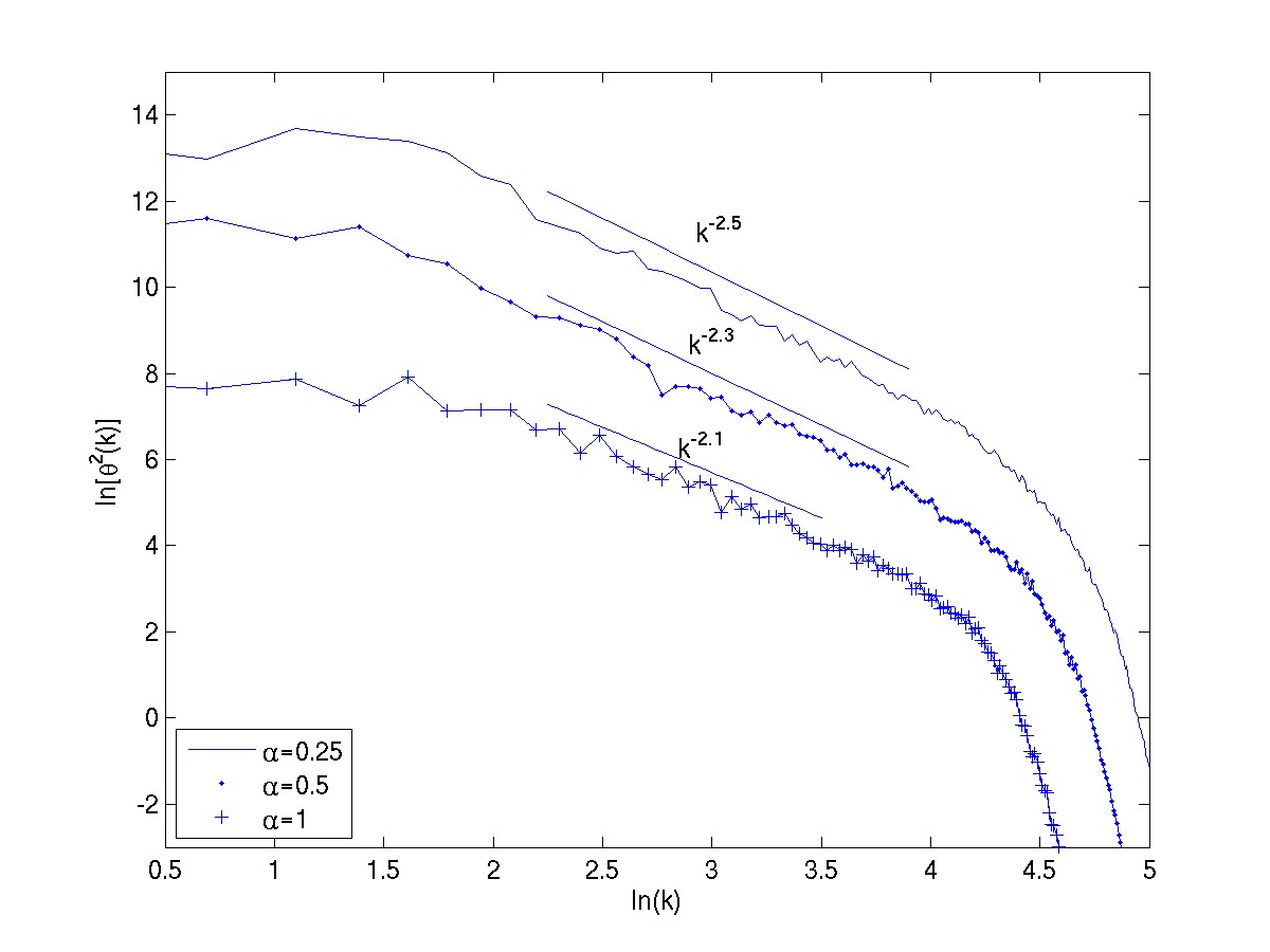
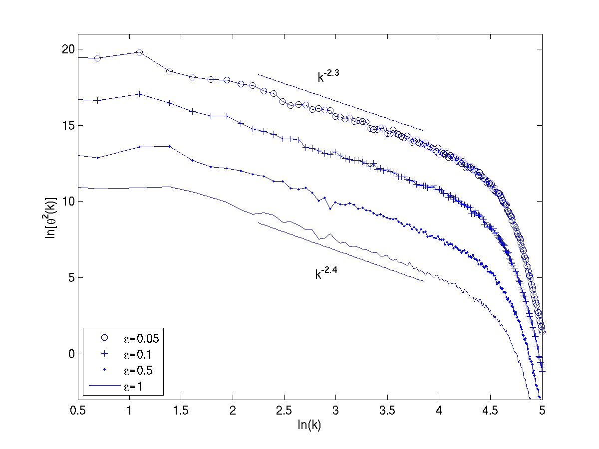
Figure 7: Enstrophy spectra in the forward weakly-local to local enstrophy transfer regime for $\epsilon=0.5$. We notice well-developed power-laws, but the slopes are significantly steeper than non-dispersive estimates. The second panel shows the same experiment for $\alpha=0.5$ but with varying $\epsilon$ ($\epsilon=0.05,0.1,0.5$ and $1$ from top to bottom). Quite clearly, the slopes are fairly insensitive to $\epsilon$. Once again, we note that our estimates of the slopes are based on invidual realizations as opposed to a temporal or ensemble average that might be more suitable at higher resolutions for accurate quantitive slopes and error estimates.

V Conclusions and discussion

We considered the evolution of a family of dispersive dynamically active scalar fields, the members of this family are characterized by the degree of locality in the $\psi-\theta$ relation. Further, the dispersive term is strong, i.e. it is preceded by the inverse of a small parameter $0<\epsilon\leq 1$. With regard to the effect of $\alpha$ on the energy/enstrophy transfer, according to the Fjortoft estimate, there is a monotonic relation between increasing $\alpha$ and the fraction of energy (enstrophy) transferred to large (small) scales. Further, the bias in energy/enstrophy partitioning increases with the spectral nonlocality of the transfer. As for the geometry of the scalar field, large isotropic coherent eddies are seen to develop from spatially un-correlated initial data for small $\alpha$, while for large $\alpha$ we see the formation of a filamentary structure (much like a small-scale passive field when advected via a large-scale smooth flow). Rhines’ argument for the spontaneous asymmetry in the streamfunction is seen to hold for all $\alpha>0.5$, while for $\alpha<0.5$ it is possible to maintain isotropy while satisfying the dual constraints of energy transfer to large scales and small frequencies. Indeed, simulations from un-correlated initial data confirm the emergence (and lack thereof) of dominant coherent zonal flows for $\alpha>0.5$ ($\alpha<0.5$) respectively footer .

Utilizing random small-scale forcing, for weakly non-local to local conditions (i.e. for $\alpha\leq 1$), we observe a clear power-law scaling in the energy spectrum, and for $\epsilon\sim 1$ the slope of the spectra agree with non-dispersive estimates. Under large-scale forcing, much like the inverse energy cascade, we see a clear forward cascade of enstrophy accompanied by a power-law scaling; though in contrast to the inverse regime, the slopes are much steeper than non-dispersive similarity hypotheses. Repeating the experiments with a dispersive term of differing strength shows that the scaling depends on $\epsilon$ in the inverse transfer regime. Specifically, along with an expected shortening of the inertial-range, at our present resolution, the associated slopes also become progressively shallower as the dispersive terms becomes stronger. On the other hand, the forward transfer regime is quite insensitive to the strength of the dispersive term, in fact we observe the enstrophy cascade slopes to be fairly universal with respect to the range of $\epsilon$ values considered.

With regard to the mathematical aspects of (1), $\alpha=0.5$ is known to be special in the sense that it represents an open problem with regard to global regularity of non-dissipative solutions (see for example Constantin, Majda & Tabak Const-NL for an analogy between front formation in SQG and finite time singularities in the 3D Euler equations). In fact, present estimates for well behaved solutions require dissipation of the form $\triangle^{\rho}$ with $\rho=0.5$ for both, the non-dispersive and dispersive cases KNV ,Kiselev . Unfortunately, regularity results for $0.5<\alpha<1$ are presently un-settled. It is unclear if the difficulty in achieving regularity (by present techniques) arises abruptly at $\alpha=0.5$ or whether one requires gradually stronger dissipation as $\alpha$ decreases from unity. Physically, this is interesting as $\alpha=0.5$ is precisely the border at which the advecting flow is of the same scale as the advected field. In fact, in the context of both the dispersive and non-dispersive cases, it would be quite interesting to know if a change in relative scales of the advecting and advected fields (as $\alpha$ crosses 0.5 from above) is connected to the deeper mathematical issue of the regularity of solutions.

Acknowledgements : We would like to acknowledge discussions with Prof. A.J. Majda (Courant Institute, NYU) and Prof. A. Kiselev (Math Department, Wisconsin, Madison). We would also like to thank the reviewers for their extensive comments. Financial support was provided by NSF CMG 0529596 and the DOE Multiscale Mathematics program (DE-FG02-05ER25703). J.S. would also like to acknowledge the hospitality of the Indian Institute of Tropical Meteorology where some of this work was conducted.

References

- (1) A.J. Majda, Introduction to PDEs and Waves for the Atmosphere and Ocean, American Mathematical Society (2003).
- (2) J-Y. Chemin et al. Mathematical Geophysics, Oxford Lecture Series in Mathematics and its Applications, Vol. 32, Oxford University Press, UK (2006).
- (3) P.B. Rhines, ”Waves and turbulence on a beta plane,” J. Fluid Mech. 69, 417 (1975).
- (4) I.M. Held, R.T. Pierrehumbert, S.T. Garner and K.L. Swanson, ”Surface quasi-geostrophic dynamics,” J. Fluid. Mech. 282, 1 (1995).
- (5) G. Holloway and M.C. Hendershott, ”Stochastic closure for nonlinear Rossby waves,” J. Fluid Mech. 82, 747 (1977).
- (6) T.G. Shepherd, ”Rossby waves and two-dimensional turbulence in a large-scale zonal jet,” J. Fluid Mech. 183, 467 (1987).
- (7) R.T. Pierrehumbert, I.M. Held and K.L. Swanson, ”Spectra of local and nonlocal two-dimensional turbulence,” Chaos, Solitons & Fractals 4, 1111 (1994).
- (8) K.S. Smith et al. ”Turbulent diffusion in the geostrophic inverse cascade,” J. Fluid Mech. 469, 13 (2002).
- (9) J. Sukhatme and R.T. Pierrehumbert, ”The decay of passive scalars under the action of single scale smooth velocity fields in bounded 2D domains : From non self similar pdf’s to self similar eigenmodes,” Phys. Rev. E, 66, 056302 (2002).
- (10) D. Fereday and P. Haynes, ”Scalar decay in two-dimensional chaotic advection and Batchelor-regime turbulence,” Phys. of Fluids, 16, 4359 (2004).
- (11) A. Majda and P. Kramer, ”Simplified models for turbulent diffusion: Theory, numerical modelling, and physical phenomena,” Physics Reports, 314 (4-5), 238 (1999).
- (12) R.H. Kraichnan, ”Intertial ranges in two-dimensional turbulence,” Phys. of Fluids 10, 1417 (1967).
- (13) T. Watanabe and T. Iwayama, ”Unified scaling theory for local and non-local transfers in generalized two-dimensional turbulence,” Journal of the Physical Society of Japan 73, 3319 (2004).
- (14) C.V. Tran, ”Nonlinear transfer and spectral distribution of energy in alpha turbulence,” Physica D, 191, 137 (2004).
- (15) C.V. Tran and J.C Bowman, ”Large-scale energy spectra in surface quasi-geostrophic turbulence,” J Fluid Mech. 526, 349 (2005).
- (16) R. Fjortoft, ”On the changes in the spectral distribution of kinetic energy for two-dimensional nondivergent flow,” Tellus 5, 225 (1953).
- (17) R. Salmon, ”Lectures on geophysical fluid dynamics,” Oxford University Press, UK (1998).
- (18) K. Hasselmann, ”A criterion for nonlinear wave stability,” J. Fluid. Mech. 30, 737 (1967).
- (19) R. Salmon, ”Geostrophic Turbulence,” in Topics in Ocean Physics, International School of Physics ”Enrico Fermi”, eds. A.R. Osborne and P. Malanotte Rizzoli, 30 (1982).
- (20) P.B. Rhines and W.R. Young, ”Homogenization of potential vorticity in planetary gyres,” J. Fluid. Mech. 122, 347 (1982).
- (21) D.G. Dritschel and M.E. McIntyre, ”Multiple jets as PV staircases : the Phillips effect and the resilience of eddy-transport barriers,” J. Atmos. Sci. 65, 855 (2008).
- (22) S. Danilov and V.M. Gryanik, ”Barotropic beta plane turbulence in a regime with strong zonal jets revisited,” J Atmos. Sci. 61, 2283 (2004).
- (23) S. Danilov and D. Gurarie, ”Scaling, spectra and zonal jets in beta-plane turbulence,” Phys. of Fluids 16, 2592 (2004).
- (24) P.S. Marcus and C. Lee, ”A model for eastward and westward jets in laboratory experiments and planetary atmospheres,” Phys. of Fluids 10, 1474 (1998).
- (25) Q. Chen, S. Chen, G.L. Eyink and D.D. Holm, ”Resonant interactions in rotating homogeneous three-dimensional turbulence,” J. Fluid. Mech. 542, 139 (2005).
- (26) M.S. Longuet-Higgins and A.E. Gill, ”Resonant interactions between planetary waves,” Proc. R. Soc. Lond. A 299, 120 (1967).
- (27) A. Babin, A. Mahalov and B. Nicolaenko, ”Global regularity of 3D rotating Navier-Stokes equations for resonant domains,” Indiana University Mathematics Journal, 48, 1133 (1999).
- (28) Y. Lee and L.M. Smith, ”A mechanism for the formation of geophysical and planetary zonal flows,” J Fluid. Mech. 576, 405 (2007).
- (29) L.M. Smith and Y. Lee, ”On near resonances and symmetry breaking in forced rotating flows at moderate Rossby number,” J Fluid. Mech. 535, 111 (2005).
- (30) S. Chen et al. ”Physical mechanism of the two-dimensional inverse energy cascade,” Phys. Rev. Lett. 96, 084502 (2006).
- (31) M.E. Maltrud and G.K Vallis, ”Energy spectra and coherent structures in forced two-dimensional and beta-plane turbulence,” J. Fluid Mech. 228, 321 (1991).
- (32) If the initial conditions and/or forcing project onto a zonal/near-zonal modes then, much like the rapid dissipation of ageostrophic components in the 3D rotating Boussinesq equations Bartello ,SS-gafd , the (catalytic) interactions will lead to the dissipation of non-zonal components by sweeping them to small scales, thereby giving the (mistaken) impression of spontaneous zonal flow generation.
- (33) P. Bartello, ”Geostrophic adjustment and inverse cascades in rotating stratified turbulence,” J. Atmos. Sci. 52, 4410 (1995).
- (34) J. Sukhatme and L.M. Smith, ”Vortical and Wave Modes in 3D Rotating Stratified Flows : Random Large Scale Forcing,” Geophys. Astrophys. Fluid Dynamics, 102, 437 (2008).
- (35) G.K. Vallis and M.E. Maltrud, ”Generation of mean flows and jets on a beta plane over topography,” J Phys. Oceanogr. 23, 1346 (1993).
- (36) G. Holloway, ”On the Spectral Evolution of Strongly Interacting Waves,” Geophys. Astrophys. Fluid Dynamics 11, 271 (1979).
- (37) A. Chekhlov et al. ”The effect of small-scale forcing on large-scale structures in two-dimensional flows,” Physica D, 98, 321 (1996).
- (38) S. Sukoriansky, N. Dikovskaya and B. Galperin, ”On the arrest of inverse energy cascade and the Rhines scale,” J. Atmos. Sci. 64, 3312 (2007).
- (39) We are using the term ”inertial-range” quite loosely in the present work.
- (40) Note that high-resolution studies of the enstrophy cascade in a stationary state (i.e. with some means of destroying long-lasting coherent vortices) are in good agreement with the anticipated scaling Borue-enstrophy , Pasquero , Boffetta .
- (41) V. Borue, ”Spectral exponents of enstrophy cascade in stationary two-dimensional homogeneous turbulence,” Phys. Rev. Lett. 71, 3967 (1993).
- (42) C. Pasquero and G. Falkovich, ”Stationary spectrum of vorticity cascade in two-dimensional turbulence,” Phys. Rev. E 65, 056305 (2002).
- (43) G. Boffetta, ”Energy and enstrophy fluxes in the double cascade of two-dimensional turbulence,” J. Fluid Mech. 589, 253 (2007).
- (44) R.T. Pierrehumbert, ”Chaotic mixing of tracer and vorticity by modulated travelling Rossby waves,” Geophys. Astrophys. Fluid Dynamics 58, 285 (1991).
- (45) G.K. Batchelor, ”Small-scale variation of convected quantities like temperature in turbulent fluids - Part I : General discussion and the case of small conductivity,” J. Fluid Mech. 5, 113 (1959).
- (46) R.H. Kraichnan, ”Convection of a passive scalar by a quasi-uniform random straining field,” J. Fluid Mech. 64, 737 (1974).
- (47) N. Schorghofer, ”Energy spectra of steady two-dimensional turbulent flows,” Phys. Rev. E, 61, 6572 (2000).
- (48) G. Falkovich and V. Lebedev, ”Nonlocal vorticity cascade in two dimensions,” Phys. Rev. E, 43, R1800 (1994).
- (49) T. Watanabe and T. Iwayama, ”Interacting scales and triad enstrophy transfers in generalized two-dimensional turbulence,” Phys. Rev. E 76, 046303 (2007).
- (50) K. Okhitani and M. Yamada, ”Inviscid and inviscid-limit behavior of a surface quasigeostrophic flow,” Phys. of Fluids, 9, 876 (1997).
- (51) J. Sukhatme and R.T. Pierrehumbert, ”Surface quasi-geostrophic turbulence : The study of an active scalar,” Chaos, 12, 439 (2002).
- (52) An intersting point raised by one of the reviewers concerns the time-scales involved in the emeregence of these coherent features. It is possible that the seemingly isotropic eddies for small will at a later time deform to yield corresponding zonal flows. We do not see this happening for fairly long times. In fact, most of the evolution in the fields occurs while the Dirichelt quotient MW-book decays rapidly in time, and these snapshots are well after a levelling off of this quotient.
- (53) A.J. Majda and X. Wang, Nonlinear Dynamics and Statistical Theories for Basic Geophysical Flows, Cambridge University Press (2006).
- (54) P. Constantin, A. Majda and E. Tabak, ”Formation of strong fronts in the 2D quasigeostrophic thermal active scalar,” Nonlinearity, 7, 1495 (1994).
- (55) A. Kiselev, F. Nazarov and A. Volberg, ”Global well posedness for the critical 2D dissipative quasi-geostrophic equation,” Inventiones Math, 167, 445 (2007).
- (56) A. Kiselev and F. Nazarov, ”Global Regularity for the Critical Dispersive Dissipative Surface Quasi-Geostrophic Equation,” preprint, (2008).