1 Introduction

The current $\Lambda$CDM standard model of cosmology is based upon General Relativity (GR) as applied to the spatially-flat Friedmann-Lemaître-Robertson-Walker (FLRW) spacetime metric together with the Weyl postulate for the energy-momentum density tensor, leading to the Friedmann equations for the 3-space scale factor [1, 2, 3, 4]. Fitting this model to the magnitude-redshift data from supernovae and gamma-ray-burst (GRB) data requires the introduction of dark energy and dark matter, and a concomitant future exponential acceleration of the universe [5]. The dark energy has been most simply interpreted as a cosmological constant $\Lambda$. Fitting the data gives $\Omega_{\Lambda}=0.73$, $\Omega_{M}=0.27$, with baryonic matter forming only some $\Omega_{b}=0.05$ of $\Omega_{M}$, so that the ‘dark matter’ component has $\Omega_{DM}=0.22$. Hence according to this GR-FLRW model the universe expansion is determined mainly by dark energy and cold dark matter, leading to the $\Lambda$CDM label. A peculiar aspect of the $\Lambda$CDM model is that the universe can only expand if the energy density is non-zero, i.e. space itself cannot expand without that energy density being present. This has been a feature of the FLRW dynamics from the beginning of cosmology. Here we derive a new cosmology which leads to, apart from other numerous tests, an expanding flat 3-space which does not require the presence of energy for that expansion. This expansion gives a parameter-free fit to the supernovae/GRB data, without invoking dark energy or dark matter. Nevertheless, if we best-fit the GR-FLRW $\Lambda$CDM model to the new cosmology dynamics over the redshift range $z\in\{0,14\}$, by varying $\Omega_{\Lambda}$, we obtain $\Omega_{\Lambda}=0.73$, $\Omega_{M}=1-\Omega_{\Lambda}=0.27$. In other words we can predict that fitting the GR-FLRW model to the data will give the parameter values exactly as reported. However the new cosmology does not predict an accelerating universe; that is merely a spurious consequence of the GR-FLRW model having the wrong functional form for its Hubble function. These results change completely our understanding of the evolution of the universe, and of its contents. Basically there is just a very small amount of conventional matter, as indeed deduced from CMB temperature fluctuation data, and a dominant expanding dynamical 3-space: both of these components of reality may be understood in a unified manner as aspects of a quantum cosmology model.

The new cosmology dynamics arises from an information-theoretic modeling of reality which does not assume a priori any notions about space or quantum matter or even gravity - these phenomena are emergent. It does however assume that time is modelled as an a priori stochastic process. From this pre-geometric system it has been shown that geometry emerges, but that this is a very complex spatial effect that requires a quantum field theoretic description, namely Quantum Homotopic Field Theory (QHFT). In this quantum matter corresponds to topological defects of a quantum-foam 3-space. QHFT is very non-local. We construct here the minimal classical-field description of the dynamical 3-space, and by generalising the Schrödinger and Dirac equations to take account of the dynamical 3-space we find that the quantum matter, in the classical limit, responds to the 3-space dynamics in a manner that we recognise as gravity - that is, we have the first derivation of gravity. As well we find the emergence of the Equivalence Principle. The minimal model for the 3-space dynamics is found to have two coupling constants, one is the long-known Newtonian $G$, the second is the fine structure constant $\alpha$. This value of $\alpha$ is determined from both bore hole $g$ anomaly data, and from the black hole mass data. This suggests the discovery of a unification in fundamental physics, that the dynamics of space as a quantum-foam and of quantum electrodynamics are both determined by $\alpha$.

A new dynamics for 3-space must be confirmed by a range of different experiments and observations, and such results are briefly reviewed herein. We see that the 3-space dynamics gives rise to a description of gravity that differs from Newtonian gravity - even in the non-relativistic limit. The differences can be extremely small, as in the solar system, and extremely large as in the case of spiral galaxies and black holes. The black holes of the new theory have very different properties from those of GR, and it is this difference that explains the rotation characteristics of spiral galaxies, and so on. As well a necessary generalisation of the Maxwell equations leads to a direct and simple account of gravitational light bending and lensing - in the case of light lensing by galactic black holes we note that these black holes generate exceptionally large lensing, which up to now has been explained as being caused by huge quantities of inferred but undetected ‘dark matter’.

Because the underlying theory is pre-geometric non-locality of the dynamics is an expected emergent property, and so the universe is predicted to have a non-local connectivity that exceeds any so far considered. It is suggested that this is possible explanation for the uniformity of the universe, and so solving the horizon problem. As well the 3-space dynamics has a uniformly expanding 3-space, when the EM and baryonic matter energy densities becomes sufficiently small, showing that the universe is flat irrespective of the energy density - this explains the flatness problem. In the GR-FLRW cosmology a flat expanding universe can only arise for an incredibly finely tuned matter density. This, it now turns out, was indicating a fundamental flaw in the GR-FLRW cosmology.

2 Information-Theoretic Pregeometry

We consider a bootstrapped self-limited information-theoretic network of ‘events’, labelled primitively by indices $i,j=1,2,3....$, by having a connectivity measure $B_{ij}\in{\cal R}$. The system evolves by stochastic iterations

$$B_{ij}\rightarrow B_{ij}-a(B+B^{-1})_{ij}+w_{ij},\mbox{\ \ }i,j=1,2,...,2N;N\rightarrow\infty$$ (1)

where $w_{ij}$ are independent random variables for each $ij$ pair and for each iteration and chosen from some probability distribution. Here $a$ is a parameter the precise value of which should not be critical but which influences the self-organisational process. Eqn.(1) behaves as a order-disorder system for emergent patterns. There is no actual distinction between nodes and links - that is merely an aspect of the bootstrapping system: the emergent system is expected to be fractal, and so nodes then are also to be understood as nothing more than connection networks. The term ‘information’ refers to the absence of any notion of substantive matter, and that only patterns or forms are actual in this ontology. The matrix inversion $B^{-1}$ involves, in principle, a knowledge of all components of $B$ - amounting to full self-referencing, while the intrinsic noise $w$ limits the efficacy of that self-referencing. This limitation to self-referencing has been related to Gödel’s theorem re formal logical systems [6] - essentially we are modelling reality by a system that acknowledges the limits to logic, that a formal syntactical logic system is not suitable for a Theory of Everything. The iterations amount to a new non-geometric model of time. Because of the noise $w$ the iterations are irreversible - so modelling a key aspect of the phenomenon of time. Clearly there is no a priori notion of geometry, space, quantum matter, etc built into this model. Nevertheless there is considerable evidence that these phenomena are emergent [6]. The essential dynamics is that of pattern formation and pattern recognition, and of the preservation over iterations of certain patterns, namely those having a non-trivial fractal topology. To briefly give some indication of this self-organisation of persistent patterns we note that at each iteration the $w$ matrix can be considered as having a block-diagonal form by considering only the rare large components. Each such block can be considered to form a random graph structure. These graphs have an intrinsic approximate geometrical property [10] - to characterise that geometry we construct the graph’s minimal spanning tree graph. Nagels [6, 7] has shown that the probability of a random connected graph having a spanning tree with $D_{k}$ nodes at link count $k$ from some arbitrarily chosen node is given by

$${\cal P}[D,L,N]\propto\frac{p^{D_{1}}}{D_{1}!D_{2}!....D_{L}!}\prod_{i=1}^{L-1}(q^{\sum_{j=0}^{i-1}{D_{j}}})^{D_{i+1}}(1-q^{D_{i}})^{D_{i+1}}$$ (2)

Here $p=1-q$ is the probability of a link between any two nodes, $N$ is the number of nodes in the random graph and $L$ is the maximum depth of the tree. The first indication of emergent geometry is obtained by numerically searching for the depth distribution $D_{1},D_{2},D_{3},...$ that maximises ${\cal P}$. The result of one such computation is shown in figure 1a. We find that the depth distribution of the minimal spanning tree of the most probable graph is well fitted by the analytic form

$$D_{k}\propto\sin^{d-1}\left(\frac{\pi k}{L}\right),\mbox{\ \ \ \ }k=1,2,....,L$$ (3)

Figure 1: (a) Points show the $D_{k}$ set and $L=40$ value found by numerically maximising ${\cal P}[D,L,N]$ for $\mbox{Log}_{10}p=-6$ for fixed $N=5000$. Curve shows $D_{k}\propto\sin^{d-1}(\frac{\pi k}{L})$ with best fit $d=3.16$ and $L=40$, showing excellent agreement, and indicating embeddability in an $S^{3}$ with some topological defects. (b) Dimensionality $d$ of the gebits as a function of the probability $p$. The linkage connections have the distribution of a 3D space, but the individual gebit components are closed compact spaces and cannot be embedded in a flat 3D background space.

The key point is that if the random graph were to be naturally embeddable in a hypersphere $S^{d}$, then we would expect this form for $D_{k}$. As shown in figure 1b this is what emerges: for low values of the probability $p$ we find that $d=3$. This shows that the random matrix that drives (1) is generating primitive geometrical structures - this is a major insight, and shows that geometry is not necessarily fundamental to reality, that it is an emergent and approximate aspect. These ‘bits of geometry’ have been termed gebits. The next stage in exposing the dynamics in (1) is that these gebits are polymerised by the inverse $B^{-1}$ process; that is, the gebits are enmeshed or cross-linked. As this is itself random this next level of structure formation is also subject to a minimal spanning tree analysis, as in (3), so the gebits themselves are polymerised into a higher-level hypersphere. This suggests that (1) generates a fractal geometrical network with the geometrical sub-components linked by discrete homotopies, as suggested by the graphic in figure 2a. As discussed below it appears that this fractal network of homotopies is describable by a quantum foam. The gebits are not preserved - the iterations in (1) essentially bring about their polymerisation and then their decay, so the gebits forming the patterns are continually replaced. So we have an ongoing processing network exhibiting a coarse-grained 3-dimensionality. For the patterns of connected gebits to be preserved, as distinct from individual gebits, the connectivity must posses a non-trivial topology, for then the topology can be preserved without preserving its individual components. It is suggested that these preserved structures are the phenomenon known as quantum matter. This brief account suggests that the information-theoretic network in (1) generates a complex geometric network with preserved topological defects embedded in an evolving 3-dimensional network which appears to be what we know of as ‘space’. See also the work in [8] on a graph theory. In the next section we discuss the observation that if the network is indeed a quantum foam system formed by quantum homotopies, then we obtain a link to the standard model of particle physics. The main focus of this work is, however, the determination of the classical-limit dynamics of the emergent quantum foam, for it is different from both the Newtonian and GR treatment of space and gravity.

3 Quantum Homotopic Field Theory: Emergent Quantum Cosmology

We suppose here that the lowest level pattern formation arising from (1) is modelled by homotopic mappings between the gebits: this is because the polymerisation of the gebits is not unique and not formally perfect as in the usual mathematical definition of a homotopy between two compact spaces, and so a functional over homotopies is perhaps a more appropriate mathematical structure to describe imperfect homotopies. This suggests that the appropriate mathematical language is that of a Quantum Homotopic Field Theory (QHFT) [6]. To construct this QHFT we introduce an appropriate configuration space, namely all the possible homotopic mappings $\pi_{\alpha\beta}:S_{\beta}\rightarrow S_{\alpha}$, with $S_{1},S_{2},..$ describing ‘clean’ or topological-defect free gebits - compact spaces of various types. Then the QHFT has the form of an iterative functional Schrödinger equation for the discrete time-evolution of a wave-functional $\Psi[\{\pi_{\alpha\beta}\},t]$

$$\Psi[\{\pi_{\alpha\beta}\},t+\Delta t]=\Psi[\{\pi_{\alpha\beta}\},t]-iH\Psi[\{\pi_{\alpha\beta}\},t]\Delta t+{\cal D}[\Psi]\Psi[\{\pi_{\alpha\beta}\},t].$$ (4)

This form arises as it is models the preservation of topologically patterned information, by means of a unitary time evolution. The last term ${\cal D}$ is the non-linear minimal manner for retaining randomness in a functional Schrödinger equation [6, 11]: unitarity is preserved, in the mean, over the time evolution, that is, the norm

$$||\Psi||=\int\prod_{\alpha\neq\beta}{\cal D}\pi_{\alpha\beta}\mu(\pi_{\alpha\beta})|\Psi[\{\pi_{\alpha\beta}\},t]|^{2}$$ (5)

is invariant under the time evolution in the mean. Here $\mu(\pi_{\alpha\beta})$ is some suitable integration measure for the homotopy $\pi_{\alpha\beta}$. Because of this term (4) is an irreversible quantum system, and is known to produce wave functional collapse. Such a term explains the Born measurement metarule in the context of the conventional Schrödinger equation [11]. In the above it produces on-going decoherence leading to a quasi-classical 3-space. The interpretation of the unitary nature of the time evolution is that in general it describes a ‘bubbling’ quantum-foam with the net strength of the connectivities preserved over time, but one without necessarily forming a quasi-classical 3-space. Occasionally however a quasi-classical 3-space arises via essentially a phase-transition - this is a Big Bang event. Once that happens the interaction term ${\cal D}$ continues to maintain that new growing phase. A key result of the work herein is the determination of the classical-limit dynamics for that process, and its comparison with the experimental and observational data.

The time step $\Delta t$ in (4) is relative to the scale of the fractal processes being explicitly described, as we are using a configuration space of mappings between prescribed gebits. At smaller scales we would need a smaller value for $\Delta t$. We now consider the form of the hamiltonian $H$. In [6] it was suggested that Manton’s non-linear ‘elasticity’ interpretation [9] of the homotopic mappings is appropriate. This then suggests that $H$ is the functional operator

$$H=\sum_{\alpha\neq\beta}h\left[\frac{\delta}{\delta\pi_{\alpha\beta}},\pi_{\alpha\beta}\right],$$ (6)

where $h[\frac{\delta}{\delta\pi},\pi]$ is the (quantum) Skyrme Hamiltonian functional operator for the system based on making fuzzy the mappings $\pi:S\rightarrow\Sigma$, by having $h$ act on wave-functionals of the form $\Psi[\pi(x);t]$. Then $H$ is the sum of pairwise embedding or homotopy hamiltonians. The corresponding functional Schrödinger equation would simply describe the time evolution of quantised Skyrmions. We shall not give the explicit form of $h$ as it is complicated, but wait to present the associated induced action.

In the absence of the non-linear ${\cal D}$ terms the time evolution in (4) can be formally written as a functional integral

$$\Psi[\{\pi\};t^{\prime}]=\int\prod_{\alpha\neq\beta}{\cal D}\tilde{\pi}_{\alpha\beta}e^{iS[\{\tilde{\pi}\}]}\Psi[\{\pi\};t],$$ (7)

where, using the continuum $t$ limit notation, the action is a sum of pairwise actions,

$$S[\{\tilde{\pi}\}]=\sum_{\alpha\neq\beta}S_{\alpha\beta}[\tilde{\pi}_{\alpha\beta}],$$ (8)

$$S_{\alpha\beta}[\tilde{\pi}] = \int_{t}^{t^{\prime}}dt^{\prime\prime}\int d^{n}x\sqrt{-g}\left[\frac{1}{2}\mbox{Tr}(\partial_{\mu}\tilde{U}\tilde{U}^{-1}\partial^{\mu}\tilde{U}\tilde{U}^{-1})\right.+$$ (9)

$$\mbox{\ \ \ \ \ \ \ \ \ \ \ \ \ \ \ \ \ \ \ \ \ \ \ \ \ }\left.\frac{1}{16}\mbox{Tr}[\partial_{\mu}\tilde{U}\tilde{U}^{-1},\partial^{\nu}\tilde{U}\tilde{U}^{-1}]^{2}\right],$$

and the now time-dependent (indicated by the tilde symbol) mappings $\tilde{\pi}$ are parametrised by $\tilde{U}(x,t)$, $\tilde{U}\in S_{\alpha}$. The metric $g_{\mu\nu}$ is that of the $n$-dimensional base space, $S_{\beta}$, in $\pi_{\alpha,\beta}:S_{\beta}\rightarrow S_{\alpha}$. As usual in the functional integral formalism the functional derivatives in the quantum hamiltonian, in (6), now manifest as the time components $\partial_{0}$ in (9), so now (9) has the form of a ‘classical’ action, and we see the emergence of ‘classical’ fields, though the emergence of ‘classical’ behaviour is a more complex process and requires the retention of the ${\cal D}$ term in (4).

A key observation is that the quantum system (7)-(9) is essentially that of the Nambu-Goldstone modes of the standard model of particle physics - by a functional change of field variables these modes may be related to a QFT involving fermionic and vector gauge fields, which are the conjectured preonic fermions and hypercolour vector fields. [6]. It is not claimed that this is a formal derivation of the standard model of particle physics from (1) - that will require much further study. See also the related work in [12]. Nevertheless it is suggestive of how a self-organising and self-limited information-theoretic system may lead to emergent behaviour describable by a quantum-theoretic formalism, and achieve that with a very generic bootstrapping system as in (1), which does not assume any emergent pattern dynamics, such as space or quantum matter, yet with the emergence of such phenomena, and in a unified manner as (7) describes both a quantum-foam dynamical 3-space as well as quantum matter. If, as suggested, a phase transition to a growing dynamical 3-space system arises, then self-organised criticality would arise, and then the details of the generic system in (1) would be hidden. In the next section we construct a minimal phenomenological classical dynamics for this quantum-foam space and discover that it predicts the phenomenon of gravity, but possessing dynamical aspects that account for the effects that, until now, have required the introduction of ‘dark matter’ and ‘dark energy’.

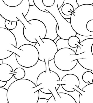
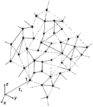
Figure 2: This is an iconic representation of how the iterative scheme in (1) generates a homotopic network (left) describable as a quantum foam. Its skeletal structure has its inherent approximate 3-dimensional connectivity displayed by an embedding in a mathematical space, such as an $E^{3}$ or an $S^{3}$, as shown on the right. The embedding space is not real - it is purely a mathematical artifact. Nevertheless this embeddability helps determine the minimal dynamics for the network, as in (10). The dynamical space is not an ether model, as the embedding space does not exist.

4 From Quantum Cosmology to Classical Dynamical 3-Space

The information-theoretic approach to modelling reality leads to an emergent structured quantum-foam ‘space’ which is 3-dimensional and dynamic, but where the 3-dimensionality is only approximate, in that if we ignore non-trivial topological aspects of the quantum foam, then it may be embedded in a 3-dimensional geometrical manifold [13]. Here the space is a real existent discrete but fractal network of relationships or connectivities, but the embedding space is purely a mathematical way of characterising the 3-dimensionality of the network. This is illustrated by the skeletal representation of the quantum foam in figure 2b - this is not necessarily local in that significant linkages can manifest between distant regions. Embedding the network in the embedding space is very arbitrary; we could equally well rotate the embedding or use an embedding that has the network translated or translating. These general requirements then dictate the minimal dynamics for the actual network, at a phenomenological level. To see this we assume at a coarse grained level that the dynamical patterns within the network may be described by a velocity field ${\bf v}({\bf r},t)$, where ${\bf r}$ is the location of a small region in the network according to some arbitrary embedding. The 3-space velocity field has been observed in at least 9 experiments [6]. For simplicity we assume here that the global topology of the network is not significant for the local dynamics, and so we embed in an $E^{3}$, although a generalisation to an embedding in $S^{3}$ is straightforward and might be relevant to cosmology. The minimal dynamics is then obtained by writing down the sum of the only three lowest-order zero-rank tensors, of dimension $1/T^{2}$, that are invariant under translation and rotation, giving

$$\nabla.\left(\frac{\partial{\bf v}}{\partial t}+({\bf v}.{\bf\nabla}){\bf v}\right)+\frac{\alpha}{8}(trD)^{2}+\frac{\beta}{8}tr(D^{2})=-4\pi G\rho$$ (10)

$$D_{ij}=\frac{1}{2}\left(\frac{\partial v_{i}}{\partial x_{j}}+\frac{\partial v_{j}}{\partial x_{i}}\right)$$ (11)

where $\rho({\bf r},t)$ is an effective matter density that may correspond to various energy densities. The embedding space coordinates provide a coordinate system or frame of reference that is convenient to describing the velocity field, but which is not real.

We see that there are only four possible terms, and so we need at most three possible constants to describe the dynamics of space: $G,\alpha$ and $\beta$. $G$ turns out to be Newton’s gravitational constant, and describes the rate of non-conservative flow of space into matter. To determine the values of $\alpha$ and $\beta$ we must, at this stage, turn to experimental and observational data. However most data involving the dynamics of space is obtained by detecting the so-called gravitational acceleration of matter, although increasingly light bending is giving new information. Now the acceleration ${\bf a}$ of the dynamical patterns in space is given by the Euler or convective expression

$${\bf a}({\bf r},t)=\lim_{\Delta t\rightarrow 0}\frac{{\bf v}({\bf r}+{\bf v}({\bf r},t)\Delta t,t+\Delta t)-{\bf v}({\bf r},t)}{\Delta t}=\frac{\partial{\bf v}}{\partial t}+({\bf v}.\nabla){\bf v}$$ (12)

and this appears in one of the terms in (10). As shown in [16] and discussed later in Sect. 9 the acceleration ${\bf g}$ of quantum matter is identical to this acceleration, apart from vorticity and relativistic effects, and so the gravitational acceleration of matter is also given by (12).

Outside of a spherically symmetric distribution of matter, of total mass $M$, we find that one solution of (10) is the velocity in-flow field given by

$${\bf v}({\bf r})=-\hat{{\bf r}}\sqrt{\frac{2GM(1+\frac{\alpha}{2}+..)}{r}}$$ (13)

but only when $\beta=-\alpha$, for only then is the acceleration of matter, from (12), induced by this in-flow of the form

$${\bf g}({\bf r})=-\hat{{\bf r}}\frac{GM(1+\frac{\alpha}{2}+..)}{r^{2}}$$ (14)

which is Newton’s Inverse Square Law of 1687 [17], but with an effective mass $M(1+\frac{\alpha}{2}+..)$ that is different from the actual mass $M$. So the success of Newton’s law in the solar system, based on Kepler’s analysis, informs us that $\beta=-\alpha$ in (10). But we also see modifications coming from the $\alpha$-dependent terms.

In general because (10) is a scalar equation it is only applicable for vorticity-free flows $\nabla\times{\bf v}={\bf 0}$, for then we can write ${\bf v}=\nabla u$, and then (10) can always be solved to determine the time evolution of $u({\bf r},t)$ given an initial form at some time $t_{0}$. The $\alpha$-dependent term in (10) (with now $\beta=-\alpha$) and the matter acceleration effect, now also given by (12), permits (10) to be written in the form

$$\nabla.{\bf g}=-4\pi G\rho-4\pi G\rho_{DM},$$ (15)

where

$$\rho_{DM}({\bf r},t)\equiv\frac{\alpha}{32\pi G}((trD)^{2}-tr(D^{2})),$$ (16)

which is an effective matter density, not necessarily non-negative, that would be required to mimic the $\alpha$-dependent spatial self-interaction dynamics. The Newtonian coupling constant $G$ is included in the definition of $\rho_{DM}$ only so that its role as an effective matter density can be illustrated - the $\alpha$ dynamics does not involves $G$. Then (15) is the differential form for Newton’s law of gravity but with an additional non-matter effective matter density. So we label this as $\rho_{DM}$ even though no matter is involved [18, 19], as this effect has been shown to explain the so-called ‘dark matter’ effect in spiral galaxies, bore hole $g$ anomalies, and the systematics of galactic black hole masses.

The spatial dynamics is non-local. Historically this was first noticed by Newton who called it action-at-a-distance. To see this we can write (10) as an integro-differential equation

$$\frac{\partial{\bf v}}{\partial t}=-\nabla\left(\frac{{\bf v}^{2}}{2}\right)+G\!\!\int d^{3}r^{\prime}\frac{\rho_{DM}({\bf r}^{\prime},t)+\rho({\bf r}^{\prime},t)}{|{\bf r}-{\bf r^{\prime}}|^{3}}({\bf r}-{\bf r^{\prime}})$$ (17)

This shows a high degree of non-locality and non-linearity, and in particular that the behaviour of both $\rho_{DM}$ and $\rho$ manifest at a distance irrespective of the dynamics of the intervening space. This non-local behaviour is analogous to that in quantum systems and may offer a resolution to the horizon problem. As well the dynamics involving $\rho_{DM}$ manifests at a a distance to a scale independent of $G$, because of the $1/G$ coefficient in $\rho_{DM}$, as noted above, and so ‘gravitational wave’ effects caused by distant activity are predicted to be much large than predicted by GR.

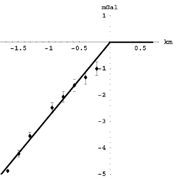
Figure 3: The data shows the gravity residuals for the Greenland Ice Shelf [20] Airy measurements of the $g(r)$ profile, defined as $\Delta g(r)=g_{Newton}-g_{observed}$, and measured in mGal (1mGal $=10^{-3}$ cm/s²) and plotted against depth in km. The borehole effect is that Newtonian gravity and the new theory differ only beneath the surface, provided that the measured above-surface gravity gradient is used in both theories. This then gives the horizontal line above the surface. Using (20) we obtain $\alpha^{-1}=137.9\pm 5$ from fitting the slope of the data, as shown. The non-linearity in the data arises from modelling corrections for the gravity effects of the irregular sub ice-shelf rock topography. The ice density is 920 kg/m³.

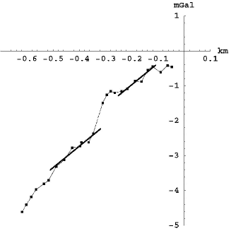
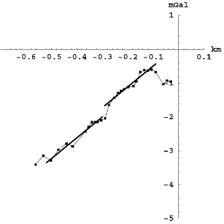
Figure 4: Gravity residuals $\Delta g(r)$ from two of the Nevada bore hole experiments [21] that give a best fit of $\alpha^{-1}=136.8\pm 3$ on using (20). Some layering of the rock is evident. The rock density is 2000 kg/m³ in the linear regions.

5 Bore Hole Anomaly: Fine Structure Constant

A recent discovery [18, 19] has been that experimental data from the bore hole $g$ anomaly has revealed that $\alpha$ is the fine structure constant, to within experimental errors: $\alpha=e^{2}/\hbar c\approx 1/137.04$. This observed anomaly is that $g(r)$ does not decrease as rapidly as predicted by Newtonian gravity or GR as we descend down a bore hole. Consider the case where we have a spherically symmetric matter distribution, at rest on average with respect to distant space, and that the in-flow is time-independent and radially symmetric. Then (10) can now be written in the form, with $v^{\prime}=dv(r)/dr$,

$$vv^{\prime\prime}+2\frac{vv^{\prime}}{r}+(v^{\prime})^{2}=-4\pi G\rho(r)-4\pi G\rho_{DM}(v(r)),$$ (18)

where now

$$\rho_{DM}(r)=\frac{\alpha}{8\pi G}\left(\frac{v^{2}}{2r^{2}}+\frac{vv^{\prime}}{r}\right).$$ (19)

The dynamics in (18) and (19) gives the anomaly to be

$$\Delta g=2\pi\alpha G\rho d+O(\alpha^{2})$$ (20)

where $d$ is the depth and $\rho$ is the density, being that of glacial ice in the case of the Greenland Ice Shelf experiments [20], or that of rock in the Nevada test site experiment [21]. Clearly (20) permits the value of $\alpha$ to be determined from the data, giving $\alpha=1/(137.9\pm 5)$ from the Greenland data, and $\alpha=1/(136.8\pm 3)$ from the Nevada data; see Figs. 3 and 4. Note that the density $\rho$ in (20) is very different for these two experiments, showing that the extracted value $\alpha$ $\approx 1/137$ is robust.

6 Minimal and Non-Minimal Black Holes: Fine Structure Constant

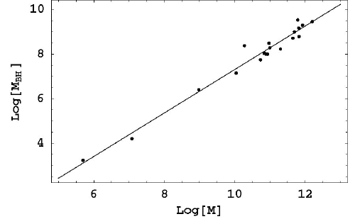
Figure 5: The data shows $\mbox{Log}_{10}[M_{BH}]$ for the black hole masses $M_{BH}$ for a variety of spherical matter systems, from Milky Way galactic clusters to spherical galaxies, with masses $M$, plotted against $\mbox{Log}_{10}[M]$, in solar masses $M_{0}$. The straight line is the prediction from (21) with $\alpha=1/137$. See [23] for references to the data.

Eqn.(18) with $\rho=0$ has exact analytic ‘black hole’ solutions, given by (22) without the $1/r$ term. There are two classes of black hole solutions - they are distinguished by how they relate to the surrounding matter. The class of minimal black holes is completely induced by the surrounding distribution of matter. For a spherically symmetric distribution of matter we find by iterating (18) and then from (19) that the total effective black hole mass is

$$M_{BH}=M_{DM}=4\pi\int_{0}^{\infty}r^{2}\rho_{DM}(r)dr=\frac{\alpha}{2}M+O(\alpha^{2})$$ (21)

This solution is applicable to the black holes at the centre of spherical star systems, where we identify $M_{DM}$ as $M_{BH}$. For these black holes the acceleration $g$ outside of the matter decreases as $1/r^{2}$. So far black holes in 19 spherical star systems have been detected and together their masses are plotted in figure 5 and compared with (21), giving again $\alpha=1/137$ [22, 23]. These solutions are called ‘black holes’ because they posses an event horizon that forbids the escape of EM radiation and matter, but that they are very different from the putative ‘black holes’ of GR. Clearly GR cannot predict the mass relation in (21) as the GR dynamics does not involve $\alpha$. The second class of black hole solutions is called non-minimal. These come into existence before subsequently attracting matter. These black holes may be primordial in that they formed directly as a consequence of the big bang before stars and galaxies, and indeed may have played a critical role in the precocious formation of galaxies. These black holes are responsible for both the rapid in-fall of matter to form rotating spiral galaxies, and also for non-Keplerian rotation characteristics of these galaxies, as discussed next. It is significant that the bore hole, black hole and (next) the spiral galaxy rotation effects are all caused by the non-local dynamics from the $\alpha$-dynamics - and so are indicative of the non-local quantum effects of the quantum cosmology.

7 Spiral Galaxy Rotation Anomaly: Fine Structure Constant

Figure 6: Data shows the non-Keplerian rotation-speed curve $v_{O}$ for the spiral galaxy NGC 3198 in km/s plotted against radius in kpc/h. Lower curve is the rotation curve from the Newtonian theory for an exponential disk, which decreases asymptotically like $1/\sqrt{r}$. The upper curve shows the asymptotic form from (24), with the decrease $\sim 1/r$ determined by the small value of $\alpha$. This asymptotic form is caused by the primordial black holes at the centres of spiral galaxies, and which play a critical role in their formation. The spiral structure is caused by the rapid in-fall towards these primordial black holes.

The black hole solutions of (18) give a direct explanation for the spiral galaxy rotation anomaly. For a non-spherical system numerical solutions of (10) are required, but sufficiently far from the centre we find an exact non-perturbative two-parameter class of analytic solutions

$$v(r)=K\left(\frac{1}{r}+\frac{1}{R_{s}}\left(\frac{R_{s}}{r}\right)^{\displaystyle{\frac{\alpha}{2}}}\right)^{1/2}$$ (22)

where $K$ and $R_{s}$ are arbitrary constants in the $\rho=0$ region, but whose values are determined by matching to the solution in the matter region. Here $R_{s}$ characterises the length scale of the non-perturbative part of this expression, and $K$ depends on $\alpha$, $G$ and details of the matter distribution. From (14) and (22) we obtain a replacement for the Newtonian ‘inverse square law’ ,

$$g(r)=\frac{K^{2}}{2}\left(\frac{1}{r^{2}}+\frac{\alpha}{2rR_{s}}\left(\frac{R_{s}}{r}\right)^{\displaystyle{\frac{\alpha}{2}}}\right),$$ (23)

in the asymptotic limit. The non-Newtonian part of this acceleration is caused by presence of a primordial ‘black hole’ at the centre of the galaxy, about which the galaxy formed: in general the ‘black holes’ from (18) have an acceleration $g\sim 1/r$, and very unlike the form $g\sim 1/r^{2}$ for the putative black holes of GR. The centripetal acceleration relation for circular orbits $v_{O}(r)=\sqrt{rg(r)}$ gives a ‘universal rotation-speed curve’

$$v_{O}(r)=\frac{K}{2}\left(\frac{1}{r}+\frac{\alpha}{2R_{s}}\left(\frac{R_{s}}{r}\right)^{\displaystyle{\frac{\alpha}{2}}}\right)^{1/2}$$ (24)

Because of the $\alpha$ dependent part this rotation-velocity curve falls off extremely slowly with $r$, as is indeed observed for spiral galaxies. An example is shown in figure 6. It was the inability of the Newtonian and Einsteinian gravity theories to explain these observations that led to the notion of ‘dark matter’. Note that in the absence of the $\alpha$-dynamics, the rotation-speed curve reduces to the Keplerian form. Nevertheless it is not clear if the form in (24) could be used to determine the value of $\alpha$ from the extensive data set of spiral galaxy rotation curves because of observational errors and intrinsic non-systematic variations in individual galaxies, unlike the data from bore holes and black holes which give independent but consistent determinations for the value of $\alpha$. We see that the 3-space dynamics (10) gives a unified account of both the ‘dark matter’ problem and the properties of ‘black holes’.

8 Generalised Maxwell Equations: Gravitational Lensing

We must generalise the Maxwell equations so that the electric and magnetic fields are excitations within the dynamical 3-space, and not of the embedding space. The minimal form in the absence of charges and currents is

$$\displaystyle{\nabla\times{\bf E}} = \displaystyle{-\mu\left(\frac{\partial{\bf H}}{\partial t}+{\bf v.\nabla H}\right)},\mbox{\ \ \ }\displaystyle{\nabla.{\bf E}={\bf 0}},$$

$$\displaystyle{\nabla\times{\bf H}} = \displaystyle{\epsilon\left(\frac{\partial{\bf E}}{\partial t}+{\bf v.\nabla E}\right)},\mbox{\ \ \ }\displaystyle{\nabla.{\bf H}={\bf 0}}$$ (25)

which was first suggested by Hertz in 1890 [24], but with ${\bf v}$ then being only a constant vector field. As easily determined the speed of EM radiation is now $c=1/\sqrt{\mu\epsilon}$ with respect to the 3-space. To see this we find plane wave solutions for (25):

$${\bf E}({\bf r},t)={\bf E}_{0}e^{i({\bf k}.{\bf r}-\omega t)}\mbox{\ \ \ \ }{\bf H}({\bf r},t)={\bf H}_{0}e^{i({\bf k}.{\bf r}-\omega t)}$$ (26)

with

$$\omega({\bf k},{\bf v})=c|\vec{{\bf k}}|+{\bf v}.{\bf k}\mbox{ \ \ \ where \ \ \ }c=1/\sqrt{\mu\epsilon}$$ (27)

Then the EM group velocity is

$${\bf v}_{EM}=\vec{\nabla}_{k}\omega({\bf k},{\bf v})=c\hat{\bf k}+{\bf v}$$ (28)

So the velocity of EM radiation ${\bf v}_{EM}$ has magnitude $c$ only with respect to the space, and in general not with respect to the observer if the observer is moving through space.

The time-dependent and inhomogeneous velocity field causes the refraction of EM radiation. This can be computed by using the Fermat least-time approximation. Then the EM ray paths ${\bf r}(t)$ are determined by minimising the elapsed travel time:

$$\tau=\int_{s_{i}}^{s_{f}}\frac{ds\displaystyle{|\frac{d{\bf r}}{ds}|}}{|c\hat{{\bf v}}_{R}(s)+{\bf v}(\bf{r}(s),t(s)|}\mbox{ \ \ with \ \ }{\bf v}_{R}=\left(\frac{d{\bf r}}{dt}-{\bf v}(\bf{r}(t),t)\right)$$ (29)

by varying both ${\bf r}(s)$ and $t(s)$, finally giving ${\bf r}(t)$. Here $s$ is a path parameter, and ${\bf v}_{R}$ is a 3-space tangent vector for the path.

In particular the in-flow in (13) causes a refraction effect of light passing close to the sun, with the angle of deflection given by

$$\delta=2\frac{v^{2}}{c^{2}}=\frac{4GM(1+\frac{\alpha}{2}+..)}{c^{2}d}$$ (30)

where $v$ is the in-flow speed at distance $d$ and $d$ is the impact parameter, here the radius of the sun. Hence the observed deflection of $8.4\times 10^{-6}$ radians is actually a measure of the in-flow speed at the sun’s surface, and that gives $v=615$km/s, in agreement with the numerical value computed for $v$ at the surface of the sun from (13).

These generalised Maxwell equations also predict gravitational lensing produced by the large in-flows, in (22), that are the new ‘black holes’ in galaxies. Until now these anomalously large lensings have been also attributed, using GR, to the presence of ‘dark matter’. One example is reported in [25] and another in [26] which is re-analaysed without requiring dark matter in [27].

9 Generalised Schrödinger Equation: Emergent Gravity and Equivalence Principle

A generalisation of the Schrödinger equation is also required [16]:

$$i\hbar\frac{\partial\psi({\bf r},t)}{\partial t}=H(t)\psi({\bf r},t),$$ (31)

where the free-fall hamiltonian is uniquely

$$H(t)=-i\hbar\left({\bf v}.\nabla+\frac{1}{2}\nabla.{\bf v}\right)-\frac{\hbar^{2}}{2m}\nabla^{2}$$ (32)

This follows from the wave function being attached to the dynamical 3-space, and not to the embedding space, and that $H(t)$ be hermitian. We can compute the acceleration of a localised wave packet using the Ehrenfest method [16], and we obtain

$${\bf g}\equiv\frac{d^{2}}{dt^{2}}\left(\psi(t),{\bf r}\psi(t)\right)=\frac{\partial{\bf v}}{\partial t}+({\bf v}.\nabla){\bf v}+(\nabla\times{\bf v})\times{\bf v}_{R}+...$$ (33)

where ${\bf v}_{R}={\bf v}_{0}-{\bf v}$ is the velocity of the wave packet relative to the local space, as ${\bf v}_{0}$ is the velocity relative to the embedding space. The vorticity term causes rotation of the wave packet. For this to occur (10) must be generaalised to the case of non-zero vorticity [6]. This vorticity effect explains the Lense-Thirring effect, and such vorticity is being detected by the Gravity Probe B satellite gyroscope experiment [30]. We see, as promised, that this quantum-matter acceleration is equal to that of the 3-space itself, as in (12). This is the first derivation of the phenomenon of gravity from a deeper theory: gravity is a quantum effect - namely the refraction of quantum waves by the internal differential motion of the substructure patterns to 3-space itself. Note that the equivalence principle has now been explained, as this ‘gravitational’ acceleration is independent of the mass $m$ of the quantum system.

10 Generalised Dirac Equation: Relativistic Effects in 3-Space

An analogous generalisation of the Dirac equation is also necessary giving the coupling of the spinor to the actual dynamical 3-space, and again not to the embedding space as has been the case up until now:

$$i\hbar\frac{\partial\psi}{\partial t}=-i\hbar\left(c{\vec{\alpha.}}\nabla+{\bf v}.\nabla+\frac{1}{2}\nabla.{\bf v}\right)\psi+\beta mc^{2}\psi$$ (34)

where $\vec{\alpha}$ and $\beta$ are the usual Dirac matrices. Repeating the analysis in (33) for the 3-space-induced acceleration we obtain

$${\bf g}=\displaystyle{\frac{\partial{\bf v}}{\partial t}}+({\bf v}.{\bf\nabla}){\bf v}+({\bf\nabla}\times{\bf v})\times{\bf v}_{R}-\frac{{\bf v}_{R}}{1-\displaystyle{\frac{{\bf v}_{R}^{2}}{c^{2}}}}\frac{1}{2}\frac{d}{dt}\left(\frac{{\bf v}_{R}^{2}}{c^{2}}\right)+...$$ (35)

which generalises (33) by having a term which limits the speed of the wave packet relative to 3-space, $|{\bf v}_{R}|$, to be $<\!c$. This equation specifies the trajectory of a spinor wave packet in the dynamical 3-space. The last term causes elliptical orbits to precess - for circular orbits $|{\bf v}_{R}|$ is independent of time.

11 Deriving the Spacetime Geodesic Formalism: Local Poincaré Symmetry

We find that (35) may be also obtained by extremising the time-dilated elapsed time

$$\tau[{\bf r}_{0}]=\int dt\left(1-\frac{{\bf v}_{R}^{2}}{c^{2}}\right)^{1/2}$$ (36)

with respect to the wave-packet trajectory ${\bf r}_{0}(t)$ [6]. This happens because of the Fermat least-time effect for waves: only along the minimal time trajectory do the quantum waves remain in phase under small variations of the path. This again emphasises that gravity is a quantum matter wave effect. We now introduce an effective spacetime mathematical construct according to the metric

$$ds^{2}=dt^{2}-(d{\bf r}-{\bf v}({\bf r},t)dt)^{2}/c^{2}=g_{\mu\nu}dx^{\mu}dx^{\nu}$$ (37)

which is of the Panlevé-Gullstrand class of metrics [28, 29]. Then we have a Local Poinacré Symmetry, namely the transformations that leave $ds^{2}$ locally invariant under a change of coordinates. As well wave effects from (10) cause ‘ripples’ in this induced spacetime, giving a different account of gravitational waves. The elapsed time in (36) may then be written as

$$\tau=\int dt\sqrt{g_{\mu\nu}\frac{dx^{\mu}}{dt}\frac{dx^{\nu}}{dt}}.$$ (38)

The minimisation of (38) leads to the geodesics of the spacetime, which are thus equivalent to the trajectories from (36), namely (35). We may introduce the standard differential geometry curvature tensor for the induced spacetime

$$R^{\rho}_{\mu\sigma\nu}=\Gamma^{\rho}_{\mu\nu,\sigma}-\Gamma^{\rho}_{\mu\sigma,\nu}+\Gamma^{\rho}_{\alpha\sigma}\Gamma^{\alpha}_{\mu\nu}-\Gamma^{\rho}_{\alpha\nu}\Gamma^{\alpha}_{\mu\sigma},$$ (39)

where $\Gamma^{\alpha}_{\mu\sigma}$ is the affine connection for the metric in (37)

$$\Gamma^{\alpha}_{\mu\sigma}=\frac{1}{2}g^{\alpha\nu}\left(\frac{\partial g_{\nu\mu}}{\partial x^{\sigma}}+\frac{\partial g_{\nu\sigma}}{\partial x^{\mu}}-\frac{\partial g_{\mu\sigma}}{\partial x^{\nu}}\right).$$ (40)

with $g^{\mu\nu}$ the matrix inverse of $g_{\mu\nu}$. In this formalism the trajectories of quantum-matter wave-packet test objects are determined by

$$\frac{d^{2}x^{\lambda}}{d\tau^{2}}+\Gamma^{\lambda}_{\mu\nu}\frac{dx^{\mu}}{d\tau}\frac{dx^{\nu}}{d\tau}=0,$$ (41)

as this is equivalent to (35). In the standard treatment of GR the geodesic for classical matter in (41) is a definition, and has no explanation. Here we see that it is finally derived, but as a quantum matter effect. Hence by coupling the Dirac spinor dynamics to the dynamical 3-space we derive the geodesic formalism of General Relativity as a quantum effect, but without reference to the Hilbert-Einstein equations for the induced metric. Indeed in general the metric of this induced spacetime will not satisfy these equations as the dynamical space involves the $\alpha$-dependent dynamics, and $\alpha$ is missing from GR. We can also define the Ricci curvature scalar

$$R=g^{\mu\nu}R_{\mu\nu}$$ (42)

where $R_{\mu\nu}=R^{\alpha}_{\mu\alpha\nu}$. In general the induced spacetime in (37) has a non-zero Ricci scalar - it is a curved spacetime. We shall compute the Ricci scalar for the expanding 3-space solution below.

We can also derive the Schwarzschild metric without reference to GR. To do this we merely have to identify the induced spacetime metric corresponding to the in-flow in (13) outside of a spherical matter system, such as the earth. Then (37) becomes

$$ds^{2}=dt^{2}-\frac{1}{c^{2}}(dr+\sqrt{\frac{2GM(1+\frac{\alpha}{2}+..)}{r}}dt)^{2}-\frac{r^{2}}{c^{2}}(d\theta^{2}+\sin^{2}(\theta)d\phi^{2})$$ (43)

Making the change of variables $t\rightarrow t^{\prime}$ and $\bf{r}\rightarrow{\bf r}^{\prime}={\bf r}$ with

$$t^{\prime}= t-\frac{2}{c}\sqrt{\frac{2GM(1{+}\frac{\alpha}{2}{+}\dots)r}{c^{2}}}+$$ (44)

$$\frac{4\ GM(1{+}\frac{\alpha}{2}{+}\dots)}{c^{3}}\,\mbox{tanh}^{-1}\sqrt{\frac{2GM(1{+}\frac{\alpha}{2}{+}\dots)}{c^{2}r}}$$

this becomes (and now dropping the prime notation)

$$ds^{2} = \left(1-\frac{2GM(1+\frac{\alpha}{2}+..)}{c^{2}r}\right)dt^{2}-\frac{1}{c^{2}}r^{2}(d\theta^{2}+\sin^{2}(\theta)d\phi^{2})$$ (45)

$$-\frac{dr^{2}}{c^{2}\left(1-{\displaystyle\frac{2GM(1+\frac{\alpha}{2}+..)}{c^{2}r}}\right)}.$$

which is one form of the the Schwarzschild metric but with the $\alpha$-dynamics induced effective mass shift. Of course this is only valid outside of the spherical matter distribution, as that is the proviso also on (13). Hence in the case of the Schwarzschild metric the dynamics missing from both the Newtonian theory of gravity and General Relativity is merely hidden in a mass redefinition, and so didn’t affect the various standard tests of GR, or even of Newtonian gravity. A non-spherical symmetry version of the Schwarzchild metric is used in modelling the Global Positioning System (GPS).

12 Supernova and Gamma-Ray-Burst Data

In the next section we show that the 3-space dynamics in (10) has an expanding space solution. The supernovae and gamma-ray bursts provide standard candles that enable observation of the expansion of the universe. To test yet further that dynamics we compare the predicted expansion against the observables, namely the magnitude-redshift data from supernovae and gamma-ray bursts. The supernova data set used herein and shown in Figs. 7 and 8 is available at [31]. Quoting from [31] we note that Davis et al. [32] combined several data sets by taking the ESSENCE data set from Table 9 of Wood–Vassey et al. (2007) [33], using only the supernova that passed the light-curve-fit quality criteria. They took the HST data from Table 6 of Riess et al. (2007) [34], using only the supernovae classified as gold. To put these data sets on the same Hubble diagram Davis et al. used 36 local supernovae that are in common between these two data sets. When discarding supernovae with $z<0.0233$ (due to larger uncertainties in the peculiar velocities) they found an offset of $0.037\pm 0.021$ magnitude between the data sets, which they then corrected for by subtracting this constant from the HST data set. The dispersion in this offset was also accounted for in the uncertainties. The HST data set had an additional 0.08 magnitude added to the distance modulus errors to allow for the intrinsic dispersion of the supernova luminosities. The value used by Wood–Vassey et al. (2007) [33] was instead 0.10 mag. Davis et al. adjusted for this difference by putting the Gold supernovae on the same scale as the ESSENCE supernovae. Finally, they also added the dispersion of 0.021 magnitude introduced by the simple offset described above to the errors of the 30 supernovae in the HST data set. The final supernova data base for the distance modulus $\mu_{obs}(z)$ is shown in Figs. 7 and 8. The gamma-ray-burst (GRB) data is from Schaefer [35].

13 Expanding Universe from Dynamical 3-Space

Let us now explore the expanding 3-space from (10). Critically, and unlike the GR-FLRW model, the 3-space expands even when the energy density is zero. Suppose that we have a radially symmetric effective density $\rho(r,t)$, modelling EM radiation, matter, cosmological constant etc, and that we look for a radially symmetric time-dependent flow ${\bf v}({\bf r},t)=v(r,t)\hat{\bf r}$ from (10) (with $\beta=-\alpha$). Then $v(r,t)$ satisfies the equation, with $v^{\prime}=\displaystyle{\frac{\partial v(r,t)}{\partial r}}$,

$$\frac{\partial}{\partial t}\left(\displaystyle{\frac{2v}{r}}+v^{\prime}\right)+vv^{\prime\prime}+2\frac{vv^{\prime}}{r}+(v^{\prime})^{2}+\frac{\alpha}{4}\left(\frac{v^{2}}{r^{2}}+\frac{2vv^{\prime}}{r}\right)=-4\pi G\rho(r,t)$$ (46)

Consider first the zero energy case $\rho=0$. Then we have a Hubble solution $v(r,t)=H(t)r$, a centreless flow, determined by

$${\dot{H}}+\left(1+\frac{\alpha}{4}\right)H^{2}=0$$ (47)

with ${\dot{H}}=\displaystyle{\frac{dH}{dt}}$. We also introduce in the usual manner the scale factor $a(t)$ according to $H(t)=\displaystyle{\frac{1}{a}\frac{da}{dt}}$. We then obtain the solution

$$H(t)=\frac{1}{(1+\frac{\alpha}{4})t}=H_{0}\frac{t_{0}}{t};\mbox{\ \ }a(t)=a_{0}\left(\frac{t}{t_{0}}\right)^{4/(4+\alpha)}$$ (48)

where $H_{0}=H(t_{0})$ and $a_{0}=a(t_{0})$. Note that we obtain an expanding 3-space even where the energy density is zero - this is in sharp contrast to the GR-FLRW model for the expanding universe, as shown below.

We can write the Hubble function $H(t)$ in terms of $a(t)$ via the inverse function $t(a)$, i.e. $H(t(a))$ and finally as $H(z)$, where the redshift observed now, $t_{0}$, relative to the wavelengths at time $t$, is $z=a_{0}/a-1$. Then we obtain

$$H(z)={H_{0}}(1+z)^{1+\alpha/4}$$ (49)

To test this expansion we need to predict the relationship between the cosmological observables, namely the relationship between the apparent energy-flux magnitudes and redshifts. This involves taking account of the reduction in photon count caused by the expanding 3-space, as well as the accompanying reduction in photon energy. To that end we first determine the distance travelled by the light from a supernova or GRB event before detection. Using a choice of embedding-space coordinate system with $r=0$ at the location of a supernova/GRB event the speed of light relative to this embedding space frame is $c+v(r(t),t)$, i.e. $c$ wrt the space itself, as noted above, where $r(t)$ is the embedding-space distance from the source. Then the distance travelled by the light at time $t$ after emission at time $t_{1}$ is determined implicitly by

$$r(t)=\int_{t_{1}}^{t}dt^{\prime}(c+v(r(t^{\prime}),t^{\prime}),$$ (50)

which has the solution on using $v(r,t)=H(t)r$

$$r(t)=ca(t)\int_{t_{1}}^{t}\frac{dt^{\prime}}{a(t^{\prime})}.$$ (51)

This distance gives directly the surface area $4\pi r(t)^{2}$ of the expanding sphere and so the decreasing photon count per unit of that surface area. However also because of the expansion the flux of photons is reduced by the factor $1/(1+z)$, simply because they are spaced further apart by the expansion. The photon flux is then given by

$${\cal F}_{P}=\frac{{\cal L}_{P}}{4\pi r(t)^{2}(1+z)}$$ (52)

where ${\cal L}_{P}$ is the source photon-number luminosity. However usually the energy flux is measured, and the energy of each photon is reduced by the factor $1/(1+z)$ because of the redshift. Then the energy flux is, in terms of the source energy luminosity ${{\cal L}_{E}}$,

$${\cal F}_{E}=\frac{{\cal L}_{E}}{4\pi r(t)^{2}(1+z)^{2}}\equiv\frac{{\cal L}_{E}}{4\pi r_{L}(t)^{2}}$$ (53)

which defines the effective energy-flux luminosity distance $r_{L}(t)$. Expressed in terms of the observable redshift $z$ this gives an energy-flux luminosity effective distance

$$r_{L}(z)=(1+z)r(z)=c(1+z)\int_{0}^{z}\frac{dz^{\prime}}{H(z^{\prime})}$$ (54)

The dimensionless ‘energy-flux’ luminosity effective distance is then given by

$$d_{L}(z)=(1+z)\int_{0}^{z}\frac{H_{0}dz^{\prime}}{H(z^{\prime})}$$ (55)

and the theory distance modulus is defined by

$$\mu(z)=5\log_{10}(d_{L}(z))+m.$$ (56)

Because all the selected supernova have the same absolute magnitude, $m$ is a constant whose value is determined by fitting the low $z$ data. The GRB magnitudes have been adjusted to match the supernovae data [35].

Using the Hubble expansion (49) in (55) and (56) we obtain the middle curves (red) in Figs. 7 and the 8, yielding an excellent agreement with the supernovae and GRB data. Note that because $\alpha/4$ is so small it actually has negligible effect on these plots. But that is only the case for the homogeneous expansion - we saw above that the $\alpha$ dynamics can result in large effects such as black holes and large spiral galaxy rotation effects when the 3-space is inhomogeneous. Hence the dynamical 3-space gives an immediate account of the universe expansion data, and does not require the introduction of a cosmological constant or ‘dark energy’, but which will be nevertheless discussed next.

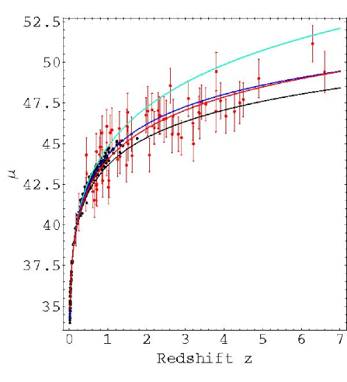
Figure 7: Hubble diagram showing the combined supernovae data from Davis et al. [32] using several data sets from Riess et al. (2007)[34] and Wood-Vassey et al. (2007)[33] (dots without error bars for clarity - see figure 8 for error bars) and the Gamma-Ray-Bursts data (with error bars) from Schaefer [35]. Upper curve (green) is ‘dark energy’ only $\Omega_{\Lambda}=1$, lower curve (black) is matter only $\Omega_{m}=1$. Two middle curves show best-fit of ‘dark energy’-‘dark-matter’ (blue) and dynamical 3-space prediction (red), and are essentially indistinguishable. However the theories make very different predictions for the future. We see that the best-fit ‘dark energy’-‘dark-matter’ curve essentially converges on the uniformly-expanding parameter-free dynamical 3-space prediction. See figure 10 for comparison out to $z=14$.

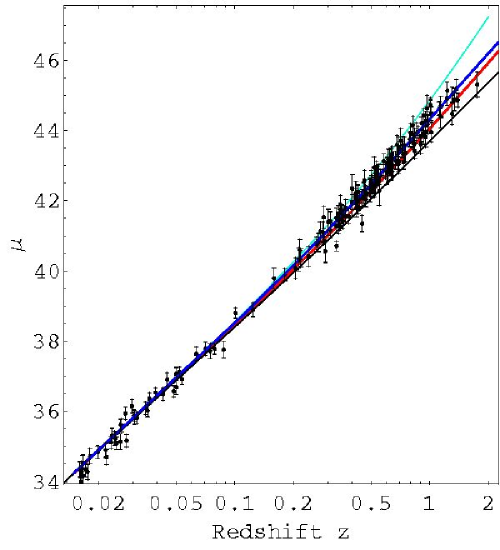
Figure 8: Hubble diagram as in figure 7 but plotted logarithmically to reveal details for $z<2$, and without GRB data. Upper curve (green) is ‘dark energy’ only $\Omega_{\Lambda}=1$. Next curve (blue) is best fit of ‘dark energy’-‘dark-matter’. Lowest curve (black) is matter only $\Omega_{m}=1$. 2nd lowest curve (red) is dynamical 3-space prediction.

14 Expanding Universe - Non-Zero Energy Density Case

When the energy density is not zero we need to take account of the dependence of $\rho(r,t)$ on the scale factor of the universe. In the usual manner we thus write

$$\rho(r,t)=\frac{\rho_{m}}{a(t)^{3}}+\frac{\rho_{r}}{a(t)^{4}}+\Lambda$$ (57)

for matter, EM radiation and the cosmological constant or ‘dark energy’ $\Lambda$, respectively, where the matter and radiation is approximated by a spatially uniform (i.e independent of $r$) equivalent matter density. We argue here that $\Lambda$ - the cosmological constant or dark energy density, like dark matter, is an unnecessary concept. We have chosen a definition for the cosmological constant $\Lambda$ so that it has the units of matter density. Then (46) becomes for $a(t)$

$$\frac{\ddot{a}}{a}+\frac{\alpha}{4}\frac{{\dot{a}}^{2}}{a^{2}}=-\frac{4\pi G}{3}\left(\frac{\rho_{m}}{a^{3}}+\frac{\rho_{r}}{a^{4}}+\Lambda\right)$$ (58)

giving

$${\dot{a}}^{2}=\frac{8\pi G}{3}\left(\frac{\rho_{m}}{a}+\frac{\rho_{r}}{a^{2}}+\Lambda a^{2}\right)-\frac{\alpha}{2}\int\frac{{\dot{a}}^{2}}{a}da+f$$ (59)

where $f$ is an integration constant. In terms of ${\dot{a}}^{2}$ this has the solution

$${\dot{a}}^{2}\!=\!\frac{8\pi G}{3}\!\!\left(\!\frac{\rho_{m}}{(1-\frac{\alpha}{2})a}\!+\!\frac{\rho_{r}}{(1-\frac{\alpha}{4})a^{2}}\!+\!\frac{\Lambda a^{2}}{(1+\frac{\alpha}{4})}\!+\!ba^{-\alpha/2}\!\right)$$ (60)

which is easily checked by substitution into (59), and where $b$ is the integration constant. Finally we obtain from (60)

$$t(a)=t(a_{0})+\int^{a}_{a_{0}}\frac{da}{\sqrt{\displaystyle{\frac{8\pi G}{3}}\left(\displaystyle{\frac{\rho_{m}}{a}+\frac{\rho_{r}}{a^{2}}}+\Lambda a^{2}+ba^{-\alpha/2}\right)}}$$ (61)

where we have re-scaled the various density parameters for notational convenience. When $\rho_{m}=\rho_{r}=\Lambda=0$, (61) reproduces the expansion in (48), and so the density terms in (60) give the modifications to the dominant purely spatial expansion, which we have noted above already gives an excellent account of the data. It is important to note that (60) has the $b$ term - the constant of integration, even when $\alpha=0$, whereas the GR-FLRW dynamics demands, effectively, $b=0$. Having $b\neq 0$ simply asserts that the 3-space can expand even when the energy density is zero - an effect missing from GR-FLRW cosmology.

From (60) we then obtain

$$H(z)^{2}={H_{0}}^{2}(\Omega_{m}(1+z)^{3}+\Omega_{r}(1+z)^{4}+\Omega_{\Lambda}+\Omega_{s}(1+z)^{2+\alpha/2})$$ (62)

where

$$H_{0}=\left(\frac{8\pi G}{3}(\rho_{m}+\rho_{r}+\Lambda+b)\right)^{1/2}$$ (63)

$$\Omega_{m}=\rho_{m}/(\rho_{m}+\rho_{r}+\Lambda+b),...$$ (64)

and so

$$\Omega_{m}+\Omega_{r}+\Omega_{\Lambda}+\Omega_{s}=1.$$ (65)

Next we discuss the strange feature of the GR-FLRW dynamics which requires a non-zero energy density for the universe to expand.

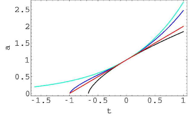
Figure 9: Plot of the scale factor $a(t)$ vs $t$, with $t=0$ being ‘now’ with $a(0)=1$, for the four cases discussed in the text, and corresponding to the plots in Figs. 7 and 8: (i) the upper curve (green) is the ‘dark energy’ only case, resulting in an exponential acceleration at all times, (ii) the bottom curve (black) is the matter only prediction, (iii) the 2nd highest curve (to the right of $t=0$) is the fitted ‘dark energy’ plus ‘dark-matter ’case (blue) showing a past deceleration and future exponential acceleration effect. The straight line plot (red) is the dynamical 3-space prediction. We see that the best-fit ‘dark energy’ - ‘dark matter’ curve closely follows the dynamical 3-space result. All plots have the same slope at $t=0$, i.e. the same value of $H_{0}$.

15 Deriving the Friedmann-Lemaître-Robertson-Walker Metric

The induced effective spacetime metric in (37) is, for the Hubble expansion,

$$ds^{2}=g_{\mu\nu}dx^{\mu}dx^{\nu}=dt^{2}-(d{\bf r}-H(t){\bf r}dt)^{2}/c^{2}$$ (66)

The occurrence of $c$ has nothing to do with the dynamics of the 3-space - it is related to the geodesics of relativistic quantum matter, as noted above. Nevertheless changing to spatial coordinate variables ${\bf r}^{\prime}$ with ${\bf r}=a(t){\bf r}^{\prime}$, and with $t^{\prime}=t$, we obtain

$$ds^{2}=g_{\mu\nu}dx^{\mu}dx^{\nu}=dt^{\prime 2}-a(t^{\prime})^{2}d{\bf r}^{\prime 2}/c^{2}$$ (67)

which is the usual Friedmann-Lemaître-Robertson-Walker (FLRW) metric in the case of a flat spatial section. However this involves a deceptive choice of spacetime coordinates. Consider the position of a galaxy located at ${\bf r}(t)$. Then over the time interval $dt$ this galaxy moves a distance $dr={\bf v}({\bf r},t)dt=H(t){\bf r}(t)dt$. In terms of the FLRW distance however the galaxy moves through distance $d{\bf r}^{\prime}=d({\bf r}(t)/a(t))=(d{\bf r}(t)-H(t){\bf r}(t))/a(t)={\bf 0}$. Hence the FLRW distances involve a dynamically determined re-scaling of the spatial distance measure so that the universe does not expand in terms of these coordinates. We now show why the GR-FLRW cosmology model needs to invoke ‘dark energy’ and ‘dark matter’ to fit the observational data.The Hilbert-Einstein (HE) equations for a spacetime metric are

$$G_{\mu\nu}\equiv R_{\mu\nu}-\frac{1}{2}Rg_{\mu\nu}=8\pi G\Lambda g_{\mu\nu}+8\pi GT_{\mu\nu}$$ (68)

where $G_{\mu\nu}$ is supposed to describe the dynamics of the spacetime manifold in the presence of an energy-momentum described by the tensor $T_{\mu\nu}$. Surprisingly, in the absence of $\Lambda$ and $T_{\mu\nu}$ the HE equation, now $G_{\mu\nu}=0$, does not have an expanding universe solution for the metric in (67).

The stress-energy tensor is, according to the Weyl postulate,

$$T_{\mu\nu}=(\rho+p)u_{\mu}u_{\nu}+pg_{\mu\nu}$$ (69)

Then with $u^{\mu}=(1,0,0,0)$ we obtain for the flat spacetime in (67) the well-known Friedmann equations

$$\frac{{\dot{a}}^{2}}{a^{2}}=\frac{8\pi G\Lambda}{3}+\frac{8}{3}\pi G\rho$$ (70)

$$\frac{{\ddot{a}}}{a}+\frac{{\dot{a}}^{2}}{2a^{2}}=4\pi G\Lambda-4\pi Gp$$ (71)

These two equations constitute the dynamical equations for the current standard model of cosmology ($\Lambda$CDM). Even in the case of zero-pressure ‘dust’, with $p=0$, these two equations are not equivalent to (58) (with $\alpha=0$ in this section). If $\rho=0,\Lambda=0$ and $p=0$ then these equations give the non-expanding universe $\dot{a}=0$, which is not the general solution to (58) which has $\dot{a}$= constant, and it is this solution which gives a parameter-free fit to the supernova/GRB redshift data. If only $p=0$ then these two equations give, first from (70), and then from (70) and (71).

$$\frac{{\dot{a}}^{2}}{2}-\frac{4\pi G\Lambda a^{2}}{3}-\frac{4\pi G\rho_{m}}{3a}=0$$ (72)

$$\frac{d}{dt}\left(\frac{{\dot{a}}^{2}}{2}-\frac{4\pi G\Lambda a^{2}}{3}-\frac{4\pi G\rho_{m}}{3a}\right)=0$$ (73)

Whence (72) requires that the integration constant from (73) must be zero - this is equivalent to demanding $b=0$ in (60). Hence according to the GR-FLRW dynamics the universe can only expand if at least one of $\Lambda$ or $\rho_{m}$ is non-zero. This amounts to not modelling space itself as a dynamical system - only the relative motion of energy/matter has any ontological meaning: this has been the main theme of spacetime modeling from the beginning. In dealing with this failure of the GR-FLRW dynamics we now show that a judicious choice of $\Omega_{\Lambda}$ and $\Omega_{m}$ can mock up the 3-space expansion, but only by introducing an extraneous and spurious acceleration.

16 Predicting the $\Lambda$CDM Parameters $\Omega_{\Lambda}$ and $\Omega_{DM}$

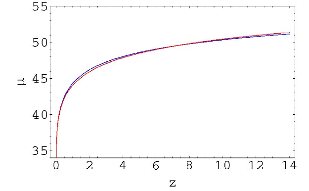
Figure 10: Comparison of GR-FLRW distance modulus $\mu(z)$ with $\Omega_{\Lambda}=0.73,\Omega_{m}=1-\Omega_{\Lambda}=0.27$, (blue plot), with distance modulus from dynamical 3-space (red plot). The small difference, which could not be distinguished by the observational data, over this redshift range demonstrates that the GR-FLRW model simulates the parameter-free uniformly-expanding dynamical 3-space prediction. Hence the ‘standard model’ values $\Omega_{\Lambda}=0.73$, $\Omega_{m}=0.27$ are predictable without reference to the actual supernovae/GRB magnitude-redshift data - there is no need to invoke ‘dark energy’ nor ‘dark matter’. The GR-FLRW model does not permit an expanding space unless there is energy residing in the space.

It is argued herein that ‘dark energy’ and ‘dark matter’ arise in the GR-FLRW cosmology because in that model space cannot expand unless there is an energy density present in the space, if that space is flat and the energy density is pressure-less. Then essentially fitting the Friedmann model $\mu(z)$ to the dynamical 3-space cosmology $\mu(z)$ we obtain $\Omega_{\Lambda}=0.73$, and so $\Omega_{m}=1-\Omega_{\Lambda}=0.27$. These values arise from a best fit for $z\in\{0,14\}$, and the quality of the fit is shown in figure 10. The actual values for $\Omega_{\Lambda}$ depend on the red-shift range used, as the Hubble functions for the GR-FLRW and dynamical 3-space have different functional dependence on $z$. These values are of course independent of the actual observed redshift data. In fitting the Friedmann dynamics to the supernovae/GRB magnitude-redshift data the best fit is $\Omega_{\Lambda}=0.73$, and so $\Omega_{m}=0.27$ [40], p40. Of course since this amount of matter is much larger than the observed baryonic matter, it is claimed that most of this matter is the so-called ‘dark matter’. Essentially the current standard model of cosmology $\Lambda$CDM is excluded from modelling a uniformly expanding dynamical 3-space, but by choice of the parameter $\Omega_{\Lambda}$ the Hubble function $H_{F}(z)$ can be made to fit the data. However $H_{F}(z)$ has the wrong functional form; when applied to the future expansion of the universe the Friedmann dynamics produces a spurious exponentially expanding universe.

17 Implications of the Supernovae and Gamma-Ray-Burst Data

As already noted above the supernovae and gamma-ray-burst data show that the universe is uniformly expanding, and that such an expansion cannot be produced by the Friedmann GR dynamics for a flat 3-space except by a judicious choice of the parameters $\Omega_{\Lambda}$ and $\Omega_{m}=1-\Omega_{\Lambda}$. Nevertheless we find that the FLRW flat 3-space spacetime metric is relevant but that it does not satisfy the Friedmann equations. We shall now illustrate this by comparing the distance moduli from various choices of the density parameters in (62). We consider four choices of parameter values with the plots shown in Figs. 7 and 8:

(i) A pure ‘dark energy’ or cosmological constant driven expansion has $\Omega_{m}=0,\Omega_{r}=0,\Omega_{\Lambda}=1,\Omega_{s}=0$. This produces a Hubble plot that causes too rapid an expansion, and indeed an exponential expansion at all epochs. This choice fails to fit the data.

(ii) A matter only expansion has $\Omega_{m}=1,\Omega_{r}=0,\Omega_{\Lambda}=0,\Omega_{s}=0$. This produces a Hubble expansion that is de-accelerating and fails to fit the data.

(iii) The $\Lambda$CDM Friedmann-GR parameters are $\Omega_{m}=0.27,\Omega_{r}=0,\Omega_{\Lambda}=0.73,\Omega_{s}=0$. They arise from a fit to the dynamical 3-space uniformly-expanding prediction as well as a best fit to the observational data. This shows that the data is implying a uniformly expanding 3-space. The Friedmann equations demand that $\Omega_{s}=0$ in the pressure-less dust case.

(iv) The zero-energy dynamical 3-space has $\Omega_{m}=0,\Omega_{r}=0,\Omega_{\Lambda}=0,\Omega_{s}=1$, as noted above. The spatial expansion dynamics alone gives a good account of the data. The data cannot distinguish between cases (iii) and (iv).

Of course the EM radiation term $\Omega_{r}$ is non-zero but small and determines the expansion during the baryongenesis initial phase, as does the spatial dynamics expansion term because of the $\alpha$ dependence.

18 Age of Universe and WMAP Data

The age of the universe is of course theory dependent. From (61) it is given in general by

$$t_{0}=\int_{0}^{1}\frac{da}{\dot{a}(t)}=\int_{0}^{\infty}\frac{dz}{(1+z)H(z)}$$ (74)

and so we must choose a form for $H(z)$, and one that models the redshift back to the Big Bang ($z=\infty$). However we only have, at best, knowledge of $H(z)$ back to say $z\approx 7$. The GR-FLRW $H(z)$ essentially fits to the 3-space form for $H(z)$ over a considerable range of $z$ values, as shown in figure 10, but not over the full $z$-range as shown in figure 9. Indeed figure 9 shows that the two $a(t)$ functions do differ, but that nevertheless they give essentially the same age for the universe. This is just an accident. However as noted when applied to the future expansion another extrapolation is employed and the GR-FLRW model predicts an exponential expansion, while the 3-space dynamics model predicts a continuing uniform expansion. From (49), with $\alpha=0$, we obtain $t_{0}=1/H_{0}$. However there will be changes to this from including effects of baryonic matter and that when the universe is inhomogeneous $\rho_{DM}$ may not be small or even positive, and would not evolve as conserved matter does as in (57).

Analysis of the CMB anisotropies by WMAP [36, 37, 38] have given results that are consistent with the $\Lambda$CDM model. However as noted herein that model involves a Hubble function that can also be matched by the Hubble function from the dynamical 3-space. So the concordance between fitting the supernovae/GRB data and the CMB data to the $\Lambda$CDM model does not imply the correctness of this model. This issue has been discussed by Efstathiou and Brown [39], and is known as the geometric degeneracy effect. What is most telling in this context is more than the existence of this degeneracy effect, but that the $\Lambda$CDM model parameters can be accurately computed without reference to the observational data, so they are purely artifacts of using the GR-FLRW $\Lambda$CDM model.

In this context we also note another geometric degeneracy, namely that if we use a FRW metric with a non-flat 3-space then the Friedmann equations now permit the term with coefficient $b$ in (60), but with $\alpha=0$, arises. This term, however, has completely different origins: in the GR-FLRW cosmology it is associated with 3-space curvature, while above it is related to the dynamics of the flat 3-space.

So from the beginning of cosmology the flawed Friedmann model of an expanding universe with a non-dynamical 3-space has been employed. The neglect of the 3-space dynamics up to now means that other methods for studying the so-called ‘dark energy’ and ‘dark matter’ need to be re-investigated: these include Baryonic Acoustic Oscillations (BAO), Galaxy Cluster Counting (GCC) and Weak Gravitational Lensing (WGL) [40]. In particular BAO analysis will be affected by the $\alpha$-dynamics term in (10) which can produce significant effects when the system is inhomogeneous. Similarly the GCC and WGL are also affected by this $\alpha$-dynamics. These effects impact on the determination of the baryonic matter content and on the computed age of the universe.

19 Ricci Curvature from the Dynamical 3-Space

We now note the form of the Ricci scalar, which is a measure of the non-flatness of the induced spacetime metric. From either (66) or (67) we obtain the Ricci scalar to be

$$R=-6\left(\frac{{\dot{a}}^{2}}{a^{2}}+\frac{\ddot{a}}{a}\right)=\frac{-96+24\alpha}{(4+\alpha)^{2}t^{2}}\neq 0$$ (75)

on using, say, expression (48) for $a(t)$. So even though the dynamical 3-space leads to the FLRW spacetime metric, with a flat 3-space, the spacetime itself is not flat. Nevertheless it is important to note that the induced spacetime has no ontological significance - it is merely a mathematical construct.

20 Conclusions

We have argued that a self-limited information-theoretic approach to modelling reality leads to an emergent quantum foam formalism, and that this in turn can be modelled, in part, by a classical dynamical 3-space. The minimal dynamics for this 3-space requires a two-parameter dynamics for that 3-space, with one being $G$ and the other being $\alpha$. That this $\alpha$ is the fine structure constant is determined from various experimental/observational data. Generalising the Schrödinger and Dirac equations then explains the phenomenon of gravity - here gravity is an emergent phenomenon arising from the wave-nature of quantum matter, and is not simply modelled as a phenomenon with known properties. The dynamical 3-space theory is then shown to explain various phenomena, including the so-called ‘dark matter’ effects - essentially these are related to the $\alpha$-dynamics that is missing from Newtonian gravity and GR. The 3-space dynamics has an expanding flat-universe solution that gives a parameter-free account of the supernovae/GRB data. This expansion occurs even when the energy density of the universe is zero. In contrast the GR-FLRW expansion dynamics only permits an expanding universe when the energy density, in the case of a pressure-less dust, is non-zero, and also essentially large. To fit the expanding 3-space solution a judicious choice of $\Omega_{\Lambda}=0.73$ and $\Omega_{m}=0.27$ in the GR-FLRW model is found, independent of the observational data. Not surprisingly these are the exact values found from fitting the GR-FLRW dynamics to the supernovae/GRB data. However a spurious aspect to this is that the GR-FLRW fit generates an anomalous exponential expansion in the future, as the GR-FLRW Hubble function has the wrong functional form. Because of the dominance of $\Omega_{\Lambda}=0.73$ and $\Omega_{m}=0.27$ the GR-FLRW dynamics has become known as the $\Lambda$CDM ‘standard’ model of cosmology. It is thus argued that the Friedmann dynamics for the universe has been flawed from the very beginning of cosmology, and that the new high-precision supernova data has finally made that evident. The derived theory of gravity does away with the need for ‘dark energy’ and ‘dark matter’. As the dynamical 3-space theory is strongly non-local we see that the universe is more connected than in previous models, and that this offers a new explanation for the uniformity of the universe, i.e. a resolution of the so-called horizon problem. The derivation of the phenomenon of gravity from the deeper Quantum Homotopic Field Theory which, it is argued, arises from the information-theoretic model for reality. The emergent gravity is seen to arise from a quantum system, and as well, displays features not in the Newtonian or the GR treatments of gravity. Hence the QHFT is a possible quantum ‘theory of everything’, including the formation of the universe via a phase transition. It thus gives us a possible quantum cosmology, and which has a ‘physics’ of the pre-universe, that is, before the beginning of a phase transition to a quasi-classical growing 3-space component.

References

- [1] Friedmann A 1922 Über die Kr mmung des Raumes, Z. Phys. 10, 377-386. (English translation in: 1999, Gen. Rel. Grav. 31, 1991-2000.)
- [2] Lemaître G 1931 Expansion of the Universe, A Homogeneous Universe of Constant Mass and Increasing Radius Accounting for the Radial Velocity of Extra-Galactic Nebulae, Monthly Notices of the Royal Astronomical Society, 91, 483-490. Translated from Lemaître G 1927 Un Univers Homogène de Masse Constante et de Rayon Croissant Rendant Compte de la Vitesse Radiale des Nébuleuses Extra-Galactiques, Annales de la Société Scientifique de Bruxelles A47, 49 56.
- [3] Robertson HP 1935 Kinematics and World Structure, Astron. J. 82, 248-301; 1936, 83, 187-200; 1936, 83, 257-271.
- [4] Walker AG 1937 On Milne’s Theory of World-Structure, Proc. London Math. Soc. 2 42, 90-127.
- [5] Perlmutter S and Schmidt BP 2003 Measuring Cosmology with Supernovae, in Supernovae and Gamma Ray Bursters, (Weiler K, Ed., Springer, Lecture Notes in Physics), 598, 195-217.
- [6] Cahill RT 2005 Process Physics: From Information Theory to Quantum Space and Matter, (Nova Science Pub., New York)
- [7] Nagels G 1983 A Bucket of Dust, Gen. Rel. and Grav. 17, 545.
- [8] Konopka T, Markopoulou F and Smolin L 2006 Quantum Graphity, arXiv:hep-th/0611197v1.
- [9] Manton NS 1987 Geometry of Skyrmions, Comm. Math. Phys. 111, 469.
- [10] Cahill RT and Klinger CM 2000 Self-Referential Noise and the Synthesis of Three-Dimensional Space, Gen. Rel. Grav., 32, 529.
- [11] Percival IC 1998 Quantum State Diffusion, (Cambridge University Press)
- [12] Bilson-Thompson, Markopoulou F and Smolin L 2007 Quantum Gravity and the Standard Model, Class. Quantum Gravity, 24, no.16, 3975-3993.
- [13] Cahill RT 2002 Process Physics: Inertia, Gravity and the Quantum, Gen. Rel. Grav., 34, 1637-1656.
- [14] Riess AG et al. 1998 Astron. J. 116, 1009.
- [15] Perlmutter S et al. 1999 Astrophys. J. 517, 565.
- [16] Cahill RT 2006 Dynamical Fractal 3-Space and the Generalised Schrödinger Equation: Equivalence Principle and Vorticity Effects, Progress in Physics, 1, 27-34.
- [17] Newton I 1687 Philosophiae Naturalis Principia Mathematica.
- [18] Cahill RT 2005 Gravity, ‘Dark Matter’ and the Fine Structure Constant, Apeiron, 12(2), 144-177.
- [19] Cahill RT 2005 ‘Dark Matter’ as a Quantum Foam In-flow Effect, in Trends in Dark Matter Research, 96-140, (ed. Val Blain J, Nova Science Pub., New York)
- [20] Ander ME et al. 1989 Test of Newton’s Inverse-Square Law in the Greenland Ice Cap, Phys. Rev. Lett., 62, 985-988.
- [21] Thomas J and Vogel P 1990 Testing the Inverse-Square Law of Gravity in Bore Holes at the Nevada Test Site, Phys. Rev. Lett., 65, 1173-1176.
- [22] Cahill RT 2005 Black Holes in Elliptical and Spiral Galaxies and in Globular Clusters, Progress in Physics, 3, 51-56.
- [23] Cahill RT 2006 Black Holes and Quantum Theory: The Fine Structure Constant Connection, Progress in Physics, 4, 44-50.
- [24] Hertz H 1890 On the Fundamental Equations of Electro-Magnetics for Bodies in Motion, Wiedemann’s Ann. 41, 369; 1962 Electric Waves, Collection of Scientific Papers, (Dover Pub., New York)
- [25] Clowe D et al. 2006 Direct Experimental Proof of the Existence of Dark Matter, Ap J, 648, L109 (C06).
- [26] Jee M et al. 2007 Discovery of a Ring-Like Dark Matter Structure in the Core of the Galaxy Cluster CL 0024+17, Ap. J., 661, 728-749.
- [27] Cahill RT 2007 Dynamical 3-Space: Alternative Explanation of the ‘Dark Matter Ring’, 4, 13-17.
- [28] Panlevé P 1921 C.R. Acad. Sci. 173, 677.
- [29] Gullstrand A 1922 Ark. Mat. Astron. Fys. 16, 1.
- [30] Cahill RT 2005 Novel Gravity Probe B Frame-Dragging Effect, Progress in Physics, 3, 30-33.
- [31] http://dark.dark-cosmology.dk/ tamarad/SN/
- [32] Davis T, Mortsell E, Sollerman J and ESSENCE 2007 Scrutinizing Exotic Cosmological Models Using ESSENCE Supernovae Data Combined with Other Cosmological Probes, astro-ph/0701510.
- [33] Wood-Vassey WM et al., 2007 Observational Constraints on the Nature of the Dark Energy: First Cosmological Results from the ESSENCE Supernovae Survey, astro-ph/0701041.
- [34] Riess AG et al. 2007 New Hubble Space Telescope Discoveries of Type Ia Supernovae at : Narrowing Constraints on the Early Behavior of Dark Energy, astro-ph/0611572.
- [35] Schaefer BE 2007 The Hubble Diagram to Redshift 6 from 69 Gamma-Ray Bursts, Ap. J. 660, 16-46.
- [36] Bennet CL et al. 2003 Wilkinson Microwave Anisotropy Probe (WMAP) Observations: Preliminary Maps and Basic Results, Astrophys. J. Suppl., 148, 1.
- [37] Verde L et al. 2003 First Year Wlikinson Microwave Anisotropy Probe (WMAP) Observations: Parameter Estimation Methodology, Astrophys. J. Suppl., 148, 195.
- [38] Kosowsky A et al. 2002 Efficient Cosmological Parameter Estimation from Microwave Background Anisotropies, Phys. Rev. D, 66, 063007.
- [39] Efstathiou G and Bond JR 1999 Cosmic Confusion: Degeneracies Among Cosmological Parameters Derived from Measurements of Microwave Background Anisotropies, Mon. Not. Roy. Astron. Soc., 304, 75-97.
- [40] Albrecht A et al. 2006 Report of the Dark Energy Task Force, arXiv:astro-ph/0609591v1.