Lie point symmetries
of difference equations and lattices

Abstract

A method is presented for finding the Lie point symmetry transformations acting simultaneously on difference equations and lattices, while leaving the solution set of the corresponding difference scheme invariant. The method is applied to several examples. The found symmetry groups are used to obtain particular solutions of differential-difference equations.

1 Introduction

Lie groups have long been used to study differential equations. As a matter of fact, they originated in that context [1, 2]. They have been put to good use to solve differential equations, to classify them, and to establish properties of their solution spaces [3, …, 8].

Applications of Lie group theory to discrete equations, like difference equations, differential-difference equations, or $q$-difference equations are much more recent [9, …, 37].

Several different approaches are being pursued. One philosophy is to consider a given system of discrete equations on a given fixed lattice and to search for a group of transformations, taking solutions into solutions, while leaving the lattice invariant. Within this philosophy different approaches differ by the restrictions imposed on the transformations and by the methods used to find the symmetries. One thing that is clear is that within this philosophy it is necessary to generalize the concept of point symmetries for difference equations, if we wish to recover all point symmetries of a differential equation in the continuous limit [9, …, 26].

A different philosophy is to consider a difference equation and a lattice as two relations involving a fixed number of points, in which we give the values of the independent and dependent variables say $x_{-},x,x_{+}$ and $u_{-},u,u_{+}$ respectively. The group transformations act on the equation and on the lattice. This philosophy was mainly developped by Dorodnitsyn and collaborators [27, …, 33]. In this approach, the given object was a Lie group and its Lie algebra. Invariants of this Lie group, depending on $x$ and $u$, calculated at a predetermined number of points were obtained. They were used to obtain invariant equations and lattices. The emphasis was on discretizing differential equations while preserving all of their point symmetries, or at least most of them.

The purpose of this article is to combine the two philosophies. More specifically, we will consider given equations on given lattices, but the lattice will also be given by some equation. We will then look for Lie point transformations, acting on both equations, and leaving the common solution sets of both equations invariant.

In Section 2 we develop the formalism necessary for calculating simultaneous symmetries of difference or differential-difference equations and lattices. Section 3 is devoted to examples of symmetries of purely difference equations, both linear and nonlinear ones. In Section 4 we also consider examples, this time of differential-difference equations. Some conclusions are drawn in the final Section 5.

2 Symmetries of differential-difference equations

2.1 The differential-difference scheme

In this article we shall only consider a restricted class of problems, for reasons of simplicity and clarity. However, the formalism involved can easily be extended to quite general systems of equations.

Thus we shall consider one scalar function $u(x,t)$ of two variables only. The variable $t$ is continuous and varies in some interval $I\subset\Re$. The variable $x$ is also continuous and varies in some interval $\tilde{I}\subset\Re$. However, $x$ will be ‘sampled’ in a set of discrete points $\{\ldots,x_{n-2}\,,\,x_{n-1}\,,\,x_{n}\,,\,x_{n+1}\,,\ldots\}$. The points $x_{k}$ are not necessarily equally spaced.

We shall study the symmetries of a pair of equations which we postulate to have the form

$$E=E\left(t,\{x_{k}\}_{k=n-n_{1}}^{n+n_{2}},\{u_{k}\}_{k=n-n_{1}}^{n+n_{2}},u_{n,t},u_{n,tt}\right) = 0$$ (1)

$$\Omega=\Omega\left(t,\{x_{k}\}_{k=n-n_{3}}^{n+n_{4}},\{u_{k}\}_{k=n-n_{3}}^{n+n_{4}}\right) = 0\ \ ,\ \ n_{i}\geq 0\,.$$ (2)

We have $k,n,n_{i}\in{Z}$, all $n_{i}$ are finite. Equations (1) is a differential equation in $t$ and a difference equation in $x$, since we define:

$$\begin{array}[]{rclcrcl}x_{n}&\equiv&x&,&x_{n-1}&\equiv&x_{n}-h_{-}(x_{n},t)\\ x_{n+1}&\equiv&x_{n}+h_{+}(x_{n},t)&,&x_{n+2}&\equiv&x_{n}+h_{+}(x_{n},t)+h_{+}(x_{n+1},t)\,,\ldots\\ u_{n}&\equiv&u(x_{n},t)&,&u_{n+k}&\equiv&u(x_{n+k},t)\,.\end{array}$$ (3)

At this stage we are not imposing any boundary conditions, so we assume that equations (1) and (2) can be shifted arbitrarily to the left and to the right. Thus, eq.(1) and (2) involve any $n_{1}+n_{2}+1$ or $n_{3}+n_{4}+1$ neighbouring points, respectively.

The fact that (1) involves only first and second derivatives and that there are no derivatives in (2) is also for simplicity only. The same goes for the fact that derivatives are evaluated at the reference point $n$ only (i.e. we do not consider terms like $\partial u(x_{n+1},t)/\partial t$).

In order to be able to consider eq.(1) and (2) as a difference scheme, we must be able to obtain $x_{n+N},u_{n+N}$ and also $x_{n-M},u_{n-M}$ ($N=\max(n_{2},n_{4}),M=\max(n_{1},n_{3})$). In other words, we impose two conditions:

$$\begin{array}[]{lcl}\det\left(\frac{\partial(E,\Omega)}{\partial(x_{n+N},u_{n+N})}\right)\not\equiv 0&,&\det\left(\frac{\partial(E,\Omega)}{\partial(x_{n-M},u_{n-M})}\right)\not\equiv 0\,.\end{array}$$ (4)

If necessary, when calculating (4) we shift one of the equations, (1) or (2), to the left or right, so that the same values $n+N$ and $n-M$ figure in both equations.

In general, we do not require that a continuous limit should exist. If it does, then eq.(1) should go into a differential equation in $x$ and $t$ and eq.(2) should go into the identity $0=0$. When taking the continuous limit it is convenient to introduce ‘discrete derivatives’, e.g.

$$u,_{x}=\frac{u_{n+1}-u_{n}}{x_{n+1}-x_{n}},\qquad u,_{\underline{x}}=\frac{u_{n}-u_{n-1}}{x_{n}-x_{n-1}},\qquad u,_{x\bar{x}}=2\frac{u,_{x}-u,_{\underline{x}}}{x_{n+1}-x_{n-1}}$$ (5)

etc. In the continuous limit we have $h_{+}(x_{k},t)\rightarrow 0\,,\,h_{-}(x_{k},t)\rightarrow 0,\,x_{n+k}\rightarrow x\,,\,u_{k}\rightarrow u(x)$ and the discrete derivatives go to the continuous ones.

A solution of the system (1), (2) will have the form $x_{n}=\Phi(n,c_{1},\ldots,c_{k})$, $u_{n}=f(x_{n},c_{1},\ldots,c_{k})$ where $c_{1},\ldots,c_{k}$ are constants needed to satisfy initial conditions and the functions $\Phi$ and $f$ are such that (1) and (2) become identities.

As a clarifying example of eqs.(1) and (2), let us consider a three point purely difference scheme, namely

$$E = \frac{u_{n+1}-2u_{n}+u_{n-1}}{(x_{n+1}-x_{n})^{2}}-u_{n}=0,$$ (6)

$$\Omega = x_{n+1}-2x_{n}+x_{n-1}=0\,.$$ (7)

The equation $\Omega=0$ determining the lattice has constant coefficients and its solution is $x_{n}=hn+x_{0}$, where $h=h_{+}=h_{-}$ and $x_{0}$ are constants. The equation $E=0$ on this lattice also has constant coefficients (since we have $x_{n+1}-x_{n}=h$) and its general solution is

$$u(x_{n})=c_{1}K_{+}^{x_{n}}+c_{2}K_{-}^{x_{n}} K_{\pm}=\left(\frac{2+h^{2}\pm h\sqrt{4+h^{2}}}{2}\right)^{1/h}\,.$$ , (8)

In the continuous limit we obtain $E=0\rightarrow u^{\prime\prime}-u=0\,,\,\Omega=0\rightarrow 0=0\,,\,u(x)=c_{1}\mathrm{e}^{x}+c_{2}\mathrm{e}^{-x}$. Eq. (7) happens to determine a regular (equally spaced) lattice. Below we shall see examples of other lattices.

2.2 Symmetries of differential-difference schemes

Let us consider a one-parameter group of local point transformations of the form

$$\tilde{x}=\Xi_{\lambda}(x,t,u)\,\,,\,\,\tilde{t}=\Gamma_{\lambda}(t)\,\,,\,\,\tilde{u}(\tilde{x},\tilde{t})=\Phi_{\lambda}(x,t,u)\,.$$ (9)

We shall require that they leave the system of equations (1), (2) invariant on the solution set of this system. Since we are interested in continuous transformations (of discrete systems), we use an infinitesimal approach and write the transformations up to order $\lambda$ as

$$\tilde{x} = x+\lambda\,\xi(x,t,u(x,t))\,,$$ (10)

$$\tilde{t} = t+\lambda\,\tau(t)\,,$$ (11)

$$\tilde{u}(\tilde{x},\tilde{t}) = u(x,t)+\lambda\,\phi(x,t,u(x,t))\ \ ,\ \ |\lambda|\ll 1\,.$$ (12)

This assumption is quite restrictive. Not only do we consider only point transformations, but we require that both $t$ and $\tilde{t}$ are continuous. No dependence, explicit or implicit, on the discretely sampled variable $x$ is allowed. Indeed, once the lattice equation is solved, we get a discrete set of points $\{x_{n}\}$and this would introduce discrete values $\tilde{t}=\tilde{t}_{n}$, which we do not allow. Moreover, the $x$-dependence of $t$, if allowed, remains unspecified, since the considered equations involve only time derivatives. This would lead to wrong results, i.e. infinite dimensional transformation groups that do not take solutions into solutions.

We must now prolong the action of the transformation (10) to the prolonged space. This space includes the derivatives $u_{t}(x,t),u_{tt}(x,t)$, the shifted points $x_{\pm}=x_{n\pm 1},\ldots$ and the function at shifted points $u_{\pm}=u(x_{\pm},t),\ldots$

It is convenient to express the invariance condition for the system (1), (2) in terms of a formalism involving vector fields and their prolongations. The vector field itself has the form

$$\hat{X}=\xi(x,t,u)\,\partial_{x}+\tau(t)\,\partial_{t}+\phi(x,t,u)\,\partial_{u}$$ (13)

with $\xi,\tau$ and $\phi$ the same as in eq.(10)–(12). The prolongation of the vector field (13) acting on the system (1), (2) is

$$\mathrm{pr}^{(M+N)}\,\hat{X}=\hat{X}+\sum_{k=n-M}^{n+N}\xi(x_{k},t,u_{k})\partial_{x_{k}}+\sum_{k=n-M}^{n+N}\phi^{(k)}\partial_{u_{k}}+\phi^{t}\partial_{u_{t}}+\phi^{tt}\partial_{u_{tt}}$$ (14)

with

$$\phi^{(k)} = \phi(x_{k},t,u_{k})$$ (15)

$$\phi^{t} = D_{t}\phi-(D_{t}\xi)\,u_{x}-(D_{t}\tau)\,u_{t}$$ (16)

$$\phi^{tt} = D_{t}\phi^{t}-(D_{t}\xi)\,u_{xt}-(D_{t}\tau)\,u_{tt}\,.$$ (17)

Thus the prolongation coefficients $\phi^{t},\phi^{tt}$ are the same as for differential equations, the coefficients $\phi^{(k)}$ are as in [10, …, 27].

The requirement that the system (1), (2) be invariant under the considered one-parameter group translates into the requirement

$$pr\hat{X}\,E\left|{}_{E=0\,,\,\Omega=0}\right.=0\ \ ,\ \ pr\hat{X}\,\Omega\left|{}_{E=0\,,\,\Omega=0}\right.=0\,.$$ (18)

In eq.(18), once the equations (1), (2) are taken into account, all involved variables are to be considered as independent. Eq.(18) are thus the determining equations for the infinitesimal coefficients $\xi,\tau$ and $\phi$.

For purely difference equations ($u_{t}$ and $u_{tt}$ absent in (1)) the procedure is the following

1. Extract $u_{n+N}$ and $x_{n+N}$ (or $u_{n-M}$ and $x_{n-M}$) from the equations (1) and (2) and substitute into eq.(18). This provides us with two functional equations for $\xi,\tau$ and $\phi$.

2. Assuming an analytical dependence of $\xi,\tau$ and $\phi$ on their own variables, we convert these two equations into differential equations by differentiating them with respect to appropriately chosen variables $u_{n+k},\,x_{n+k}$. Use the fact that the coefficients $\xi,\tau$ and $\phi$ depend on $x$ and $u$ evaluated at one point only to simplify the equations. Differentiate sufficiently many times to obtain differential equations that we can integrate.

3. Solve the differential equations, substitute back into the two original functional equations and solve them.

For differential-difference equations, we solve for the highest derivative (in our case $u_{tt}$) and for either $x_{n+N}$, or $u_{n+N}$ (or $x_{n-M}$ or $u_{n-M}$) and substitute into eq.(18). In this case, the determining equation will be a polynomial expression in the derivatives of $u$ with respect to $t$ (in our case $u_{t}$ only) and all their coefficients must vanish. For the remaining terms, which depend on shifted variables, we proceed as in the case of purely difference equations.

3 Examples of symmetries of difference equations

We shall give several examples of the calculation of symmetries acting on difference schemes. They will involve either three or four points on a lattice. Equations (1) and (2) simplify to

$$E(x,x_{-},x_{+},x_{++},u,u_{-},u_{+},u_{++})=0$$ (19)

$$\Omega(x,x_{-},x_{+},x_{++},u,u_{-},u_{+},u_{++})=0$$ (20)

for a four point scheme. A three point scheme is obtained if $E$ and $\Omega$ are independent of $x_{++}$ and $u_{++}$. Here $x=x_{n}$ is the reference point and $x_{-}=x_{n-1},\,x_{+}=x_{n+1},\,x_{++}=x_{n+2}$ and similarly for $u$.

The prolongation (14) of the vector field simplifies to

$$\begin{array}[]{rcl}pr\hat{X}&=&\xi(x,u)\partial_{x}+\phi(x,u)\partial_{u}+\xi(x_{-},u_{-})\partial_{x_{-}}+\xi(x_{+},u_{+})\partial_{x_{+}}+\phi(x_{-},u_{-})\partial_{u_{-}}\\[8.61108pt] &&+\xi(x_{++},u_{++})\partial_{x_{++}}+\phi(x_{+},u_{+})\partial_{u_{+}}+\phi(x_{++},u_{++})\partial_{u_{++}}\ .\end{array}$$ (21)

(for three point schemes we drop the $x_{++},\,u_{++}$ terms).

A symmetry classification of three point schemes was provided in a recent article [35]. Here we solve a different problem. The equations and lattices are given and we determine their symmetries.

3.1 Polynomial nonlinearity on a uniform lattice

Let us consider the nonlinear ordinary differential equation

$$u_{xx}-u^{N}=0\ \ ,\ \ N\not\equiv 0,1\,.$$ (22)

A straightforward calculation shows that for $N\not\equiv-3$ eq.(22) is invariant under a two-dimensional Lie group, the Lie algebra of which is spanned by

$$\hat{P}=\partial_{x}\ \ ,\ \ \hat{D}=(N-1)x\partial_{x}-2u\partial_{u}\,.$$ (23)

For $N=-3$ the symmetry algebra is $sl(2,\Re)$ with a basis

$$\hat{P}=\partial_{x}\ \ ,\ \ \hat{D}=2x\partial_{x}+u\partial_{u}\ \ ,\ \ \hat{C}=x^{2}\partial_{x}+xu\partial_{u}\,.$$ (24)

A natural way to discretize eq.(22) is to use a uniform lattice and put

$$E = \frac{u_{+}-2u+u_{-}}{(x_{+}-x)^{2}}-u^{N}=0$$ (25)

$$\Omega = x_{+}-2x+x_{-}=0\,.$$ (26)

Let us now apply the symmetry algorithm (18). The condition $prX\,\Omega=0$ for $E=0,\,\Omega=0$ implies

$$\xi(2x-x_{-},(x-x_{-})^{2}u^{N}+2u-u_{-})-2\xi(x,u)+\xi(x_{-},u_{-})=0\,.$$ (27)

Differentiating first by $\partial_{u_{-}}$, then by $\partial_{u}$ we obtain

$$-\xi_{u_{+}}(2x-x_{-},(x-x_{-})^{2}u^{N}+2u-u_{-})+\xi_{u_{-}}(x_{-},u_{-}) = 0$$ (28)

$$\left[N(x-x_{-})^{2}\,u^{N-1}+2\right]\,\xi_{u_{+}u_{+}}(2x-x_{-},(x-x_{-})^{2}u^{N}+2u-u_{-}) = 0\,.$$ (29)

Eq.(29) implies that $\xi$ is linear in $u$

$$\xi(x,u)=a(x)u+b(x)\,.$$ (30)

Eq.(28) reduces to $a(x_{+})=a(x)$, i.e. $a$ is a constant. Substituing these results into eq.(27) we obtain

$$a\,[u_{+}-2u+u_{-}]+b(x_{+})-2b(x)+b(x_{-})=0\,.$$ (31)

This implies $a=0$ and

$$b(x_{+})-2b(x)+b(x_{-})=0\,.$$ (32)

Differentiating successively with respect to $x$ and $x_{-}$ we find $b_{x_{+}x_{+}}(x_{+})=0$, i.e.

$$b(x)=b_{1}x+b_{0}\,.$$ (33)

Thus, the invariance of eq.(26) implies $\xi=b_{1}x+b_{0}$ with $b_{1},\,b_{0}$ constants. The function $\phi(x,u)$ is restricted by the requirement $prX\,E=0$ for $E=0,\,\Omega=0$. This invariance condition is given by

$$\begin{array}[]{l}\phi(2x-x_{-},(x-x_{-})^{2}u^{N}+2u-u_{-})-2\phi(x,u)+\phi(x_{-},u_{-})\\[8.61108pt] -(x-x_{-})^{2}[N\phi(x,u)u^{N-1}+2b_{1}u^{N}]=0\,.\end{array}$$ (34)

We successively differentiate this equation with respect to $u_{-}$ and $u$ and we obtain

$$-\phi_{u_{+}}(x_{+},u_{+})+\phi_{u_{-}}(x_{-},u_{-}) = 0$$ (35)

$$\phi_{u_{+}u_{+}}(x_{+},u_{+}) = 0\,.$$ (36)

These two equations require that $\phi=\phi_{1}u+\phi_{0}(x)$ with $\phi_{1}$ a constant. Substituing back into eq.(34) we obtain the remaining determining equation

$$\phi_{0}(2x-x_{-})-2\phi_{0}(x)+\phi_{0}(x_{-})-(x-x_{-})^{2}[(N-1)\phi_{1}+2b_{1}]u^{N}-N(x-x_{-})^{2}\phi_{0}u^{N-1}=0$$ (37)

Since we have $N\not\equiv 0,1$ eq.(37) implies $\phi_{0}(x)=0$ and $\phi_{1}(1-N)=2b_{1}$. Finally, we obtain the symmetry algebra of the difference system (25), (26). It is $2$-dimensional and coincides with the algebra (23) of the differential equation (22), the continuous limit of eq.(25).

Notice that the case $N=-3$ is not distinguished from the generic case. As a matter of fact, no difference equation on a uniform lattice can be invariant under the $SL(2,\Re)$ group corresponding to the algebra (24). A basis for the difference invariants of this algebra in the space $\{x,x_{-},x_{+},u,u_{-},u_{+}\}$ is

$$\rho_{1}=\frac{h_{-}u_{+}}{(h_{+}+h_{-})u}\ \ ,\ \ \rho_{2}=\frac{h_{+}u_{-}}{(h_{+}+h_{-})u}\ \ ,\ \ \rho_{3}=\frac{h_{+}h_{-}}{(h_{+}+h_{-})u^{2}}$$ (38)

where $h_{+}$ and $h_{-}$ are defined as $h_{+}=x_{+}-x,\,h_{-}=x-x_{-}$, and no function of $x$, $x_{+}$ and $x_{-}$ alone can be set equal to a constant. An $SL(2,\Re)$ invariant scheme must be constructed out of these invariants. For instance, an invariant scheme approximating eq.(22) for $N=-3$ is

$$\frac{h_{-}(u_{+}-u)-h_{+}(u-u_{-})}{h_{+}h_{-}(h_{+}+h_{-})} = \frac{2h_{+}h_{-}}{(h_{+}+h_{-})^{2}}\frac{1}{u^{3}}\ \ ,\ \ h_{-}u_{+}=h_{+}u_{-}\,.$$ (39)

3.2 Discrete versions of linear second order equations

3.2.1 Discretization of $u_{xx}=u$

Consider the ordinary differential equation

$$u_{xx}=u.$$ (40)

Like every second order linear ODE, it is invariant under $SL(3,\Re)$ with the Lie algebra realized in this case by the vector fields

$$\begin{array}[]{c}\hat{X}_{1}=\partial_{x}\ ,\ \hat{X}_{2}=u\partial_{u}\ ,\ \hat{X}_{3}=e^{x}\partial_{u}\ ,\ \hat{X}_{4}=e^{-x}\partial_{u}\ ,\ \hat{X}_{5}=e^{2x}(\partial_{x}+u\partial_{u}),\\[8.61108pt] \hat{X}_{6}=ue^{x}(\partial_{x}+u\partial_{u})\ ,\ \hat{X}_{7}=e^{-2x}(\partial_{x}-u\partial_{u})\ ,\ \hat{X}_{8}=ue^{-x}(\partial_{x}-u\partial_{u})\,.\end{array}$$ (41)

A very straightford discretization of eq.(40) on a uniform lattice is

$$\frac{u_{+}-2u+u_{-}}{(x_{+}-x)^{2}} = u,$$ (42)

$$x_{+}-2x+x_{-} = 0\,.$$ (43)

Applying the same procedure to the system (42), (43) that was applied to the system (25), (26) (with $N\not\equiv 0,1$), we again obtain a $2$-dimensional symmetry algebra

$$\hat{P}=\partial_{x}\ \ ,\ \ \hat{D}=u\partial_{u}\,.$$ (44)

At first glance the absence of symmetries of the form $\phi(x)\partial_{u}$, representing the linear superposition principle, seems surprising. However, viewed as a system of two equations, the system (42), (43) is really nonlinear. Eq.(43) defines a uniform lattice with an arbitrary step $h=x_{+}-x=x-x_{-}$, where the step $h$ can be scaled by a dilatation of $x$.

An alternative approach to the system (42), (43) is to first integrate eq. (43) once, thus fixing the step on the $x$-axis. The system (42), (43) is then replaced by the equation

$$\frac{u_{+}-2u+u_{-}}{h^{2}}=u\ ,$$ (45)

where $h=x_{+}-x=x-x_{-}$ is a fixed (non-scalable) constant. The symmetry algorithm described in Section 2 and applied in Section 3.1 yields a four-dimensional symmetry algebra

$$\hat{P}=\partial_{x}\ \ ,\ \ \hat{D}=u\partial_{u}\ \ ,\ \ \hat{S}_{1}=K_{+}^{x}\partial_{u}\ \ ,\ \ \hat{S}_{2}=K_{-}^{x}\partial_{u}$$ (46)

with $K_{\pm}$ as in eq.(8). The symmetries $\hat{S}_{1},\,\hat{S}_{2}$ represent the linear superposition formula for the linear system (45).

We mention that eq.(40) (and any linear ODE) can be discretized in a manner that exactly preserves all of its solutions. To do this we must preserve a subalgebra of the symmetry algebra of the ODE, containing the elements corresponding to the linear superposition formula. In our case these are $\hat{X}_{3}$ and $\hat{X}_{4}$ of eq.(41). Let us consider the subalgebra $\{\hat{X}_{1},\ldots,\hat{X}_{6}\}$. Its second order discrete prolongation allows no invariants. It does however allow an invariant manifold, namely

$$I=ue^{-x}(e^{-2x_{+}}-e^{-2x_{-}})+u_{+}e^{-x_{+}}(e^{-2x_{-}}-e^{-2x})+u_{-}e^{-x_{-}}(e^{-2x}-e^{-2x_{+}})=0\,.$$ (47)

The expression

$$S=\frac{e^{-2x}-e^{-2x_{-}}}{e^{-2x_{+}}-e^{-2x}}$$ (48)

is an invariant on the manifold (47).

Indeed, we have

$$\begin{array}[]{c}(\hat{X}_{1}+3\hat{X}_{2})\,I=0\ \ ,\ \ \hat{X}_{3}\,I=\hat{X}_{4}\,I=\hat{X}_{5}\,I=\hat{X}_{6}\,I=0\ \ ,\ \ \hat{X}_{2}\,I=I,\\[8.61108pt] \hat{X}_{i}\,S=0\ \ (i=1,\ldots,5)\ \ ,\ \ \hat{X}_{6}\,S=\frac{2\,I}{(e^{-2x_{+}}-e^{-2x})^{2}}\,,\end{array}$$ (49)

so that we have

$$\hat{X}_{i}\,I\left|{}_{I=0}=\right.0\ \ ,\ \ \hat{X}_{i}\,S\left|{}_{I=0}=\right.0\ \ ,\ \ i=1,\ldots,6\,.$$ (50)

A uniform lattice, to first order in $h$ and an equation with (40) as its continuous limit, is obtained by putting

$$S=1\ \ \ ,\ \ \ \frac{e^{3x}\,I}{2h^{3}}=0\,.$$ (51)

Eq.(51), or $I=0$, has $u=e^{x}$ and $u=e^{-x}$ as solutions and the general solution is

$$u=c_{1}e^{x}+c_{2}e^{-x}\,,$$ (52)

just as in the continuous case (40).

To check this, let us solve the system $S=1$, $I=0$ directly, with $I$ and $S$ given in eq. (47) and (48), respectively. We linearize $S=1$ by a change of variables and obtain:

$$z=e^{-2x}\ \ ,\ \ z_{+}-2z+z_{-}=0.$$ (53)

The solution is:

$$z_{n}=c_{3}n+c_{4},\,\ \ x_{n}=-\frac{1}{2}\ln(c_{3}n+c_{4}),$$ (54)

so that the lattice in $x$ is logarithmic ( $c_{3}$ and $c_{4}$ are integration constants). On this lattice eq.(47) reduces to

$$2u\sqrt{c_{3}n+c_{4}}-u_{+}\sqrt{c_{3}(n+1)+c_{4}}-u_{-}\sqrt{c_{3}(n-1)+c_{4}}=0.$$ (55)

To solve this linear equation we put $u(x)=e^{x}f(x)$ or, on the lattice

$$u(x_{n})=\frac{1}{\sqrt{c_{3}n+c_{4}}}f(x_{n}),$$ (56)

so that $f(x)$ satisfies

$$f(x_{+})-2f(x)+f(x_{-})=0.$$ (57)

We write the general solution of eq.(57) as

$$f(x_{n})=f\circ x(n)=A\,n+B\ .$$ (58)

By rewriting $A$ and $B$ in terms of the new integration constants $c_{1}$ and $c_{2}$, i.e. by putting $A=c_{2}\,c_{3}$ and $B=c_{2}\,c_{4}+c_{1}$, we obtain the general solution of the system (51) as

$$u=\frac{c_{1}}{\sqrt{c_{3}n+c_{4}}}+c_{2}\sqrt{c_{3}n+c_{4}}=c_{1}\mathrm{e}^{x}+c_{2}\mathrm{e}^{-x}$$ (59)

in full agreement with eq.(52).

3.2.2 Discrete version of $u_{xx}=1$

Let us consider the simplest 3 point difference scheme for the ODE $u_{xx}=1$

$$\frac{u_{+}-2u+u_{-}}{(x_{+}-x)^{2}}=1\ \ ,\ \ x_{+}-2x+x_{-}=0\,.$$ (60)

Applying the prolonged vector field to these equations and eliminating $x_{+}$ and $u_{+}$, we obtain two equations

$$\xi(2x-x_{-},(x-x_{-})^{2}+2u-u_{-})-2\xi(x,u)+\xi(x_{-},u_{-})=0,$$ (61)

$$\phi(2x-x_{-},(x-x_{-})^{2}+2u-u_{-})-2\phi(x,u)+\phi(x_{-},u_{-})=$$

$$2(x-x_{-})\left[\xi(2x-x_{-},(x-x_{-})^{2}+2u-u_{-})-\xi(x,u)\right]\,.$$ (62)

We first concentrate on eq.(61). Taking the second derivative with respect to $u$ and $u_{-}$ we find that $\xi$ is linear in $u$. Substituing back into (61) and differentiating with respect to $x$ and $x_{-}$ we find

$$\xi(x,u)=\alpha(u-\frac{x^{2}}{2})+\beta_{1}x+\beta_{0}$$ (63)

where $\alpha,\,\beta_{1}$ and $\beta_{0}$ are constants. Substituing $\xi$ into eq.(62) and solving for $\phi$ in a similar manner, we obtain:

$$\phi(x,u)=\alpha(xu-\frac{x^{3}}{2})+c(u-\frac{x^{2}}{2})+\beta_{1}x^{2}+\beta_{2}x+\beta_{3}.$$ (64)

Finally, a basis for the symmetry algebra of the system (60) is

$$\begin{array}[]{c}\hat{X}_{1}=\partial_{x}\ ,\ \hat{X}_{2}=\partial_{u}\ ,\ \hat{X}_{3}=x\partial_{u}\ ,\ \hat{X}_{4}=x\partial_{x}+x^{2}\partial_{u},\\[8.61108pt] \hat{X}_{5}=(u-\frac{x^{2}}{2})\partial_{u}\ ,\ \hat{X}_{6}=(u-\frac{x^{2}}{2})\partial_{x}+(u-\frac{x^{2}}{2})x\partial_{u}\,.\end{array}$$ (65)

It is easy to check that this Lie algebra is isomorphic to the general affine Lie algebra $gaff(2,\Re)$. This is the symmetry algebra of the scheme [35]

$$w_{+}-2w+w_{-}=0\ \ ,\ \ t_{+}-2t+t_{-}=0\,.$$ (66)

Indeed the system (60) is transformed into (66) by putting

$$u=w+\frac{t^{2}}{2}\ \ ,\ \ x=t\,.$$ (67)

3.3 Discrete versions of the equation $u_{xxx}=0$

The symmetry algebra of the ODE $u_{xxx}=0$ is $7$-dimensional. A basis for this algebra is

$$\begin{array}[]{c}\hat{X}_{1}=\partial_{x}\ ,\ \hat{X}_{2}=\partial_{u}\ ,\ \hat{X}_{3}=x\partial_{x}\ ,\ \hat{X}_{4}=u\partial_{u}\ ,\ \hat{X}_{5}=x\partial_{u},\\[8.61108pt] \hat{X}_{6}=x^{2}\partial_{u}\ ,\ \hat{X}_{7}=x^{2}\partial_{x}+2xu\partial_{u}\,.\end{array}$$ (68)

The generators $\hat{X}_{2},\,\hat{X}_{5},\,\hat{X}_{6}$ correspond to the linear superposition principle. We can add $u=c_{2}x^{2}+c_{1}x+c_{0}$ to any solution and indeed, this itself is the general solution.

Let us now consider discretizations of this ODE.

3.3.1 Discretization on a uniform lattice

We consider the system

$$E = u_{++}-3u_{+}+3u-u_{-}=0,$$ (69)

$$\Omega_{1} = x_{+}-2x+x_{-}=0.$$ (70)

The lattice is uniform, since the general solution of (70) is $x_{n}=hn+x_{0}$ with $h$ and $x_{0}$ constants. Eq.(70) must be shifted once to the right to obtain $x_{++}$.

The prolonged vector fields have the form (21). We apply the same method as in Section 3.2. to obtain the symmetry algebra of the system (69), (70). The result is a $6$-dimensional Lie algebra generated by $\{\hat{X}_{1}\,,\,\hat{X}_{2}\,,\,\hat{X}_{3}\,,\,\hat{X}_{4}\,,\,\hat{X}_{5}\,,\,\hat{X}_{6}\}$ of eq.(68). The system hence has exactly the same solutions as the ODE $u_{xxx}=0$, however the lattice is not invariant under the projective transformations generated by $\hat{X}_{7}$.

3.3.2 Discretization on a four point lattice

We take the equation (69) on the lattice

$$\Omega_{2}=x_{++}-3x_{+}+3x-x_{-}=0\,.$$ (71)

The lattice given by equation (71) is not uniform but satisfies $x_{n}=L_{2}n^{2}+L_{1}n+L_{0}$, where $L_{i}$ are constants. We assume $L_{2}\not\equiv 0$, otherwise the lattice is the same as for $\Omega_{1}=0$.

The symmetry algebra in this case is given by

$$\{\hat{X}_{1}\,,\,\hat{X}_{2}\,,\,\hat{X}_{3}\,,\,\hat{X}_{4}\,,\,\hat{X}_{5}\,,\,\hat{Y}=u\partial_{x}\}$$ (72)

with $\hat{X}_{1},\ldots,\hat{X}_{5}$ as in eq.(68). Thus $\hat{X}_{6}$ of (68) is absent. This reflects the fact that $u=x^{2}$ is not an exact solution on the lattice $\Omega_{2}=0$. Indeed, if we take $L_{2}=1$ and $L_{1}=L_{0}=0$ in eq.(68) we have $u=n^{4}$ which would solve a fourth order equation, not however equation (69).

3.3.3 Discretization preserving the entire symmetry group

The third prolongation of the algebra (68) acts on an 8-dimensional space with coordinates $(x\,,\,x_{+}\,,\,x_{++}\,,\,x_{-}\,,\,u\,,\,u_{+}\,,\,u_{++}\,,\,u_{-})$. If the 7 prolonged fields are linearly independent, they will allow only one invariant. This invariant can be calculated directly. It lies entirely in the subspace $\{x\,,\,x_{+}\,,\,x_{++}\,,\,x_{-}\}$ and is given by the anharmonic ratio of four points, namely

$$\frac{(x_{++}-x)(x_{+}-x_{-})}{(x-x_{-})(x_{++}-x_{+})}=K\,.$$ (73)

This is the invariant of the projective action of $sl(2,\Re)$ on the real line $\Re$, given by the $\partial_{x}$ part of the subalgebra $\{\hat{X}_{1}\ ,\ \hat{X}_{3}\ ,\ \hat{X}_{7}\}$ of the algebra (68). Eq.(73) provides us with a lattice. The invariant equation is obtained by requiring that the third prolongation of $(\hat{X}_{1},\ldots,\hat{X}_{7})$ be linearly connected on some manifold. This manifold is given by the condition

$$\begin{array}[]{lcl}I=&-&(u_{+}-u)(x_{++}-x)(x-x_{-})(x_{++}-x_{-})\\[8.61108pt] &+&(u_{++}-u)(x_{+}-x)(x-x_{-})(x_{+}-x_{-})\\[8.61108pt] &+&(u-u_{-})(x_{+}-x)(x_{++}-x)(x_{++}-x_{+})=0\,.\end{array}$$ (74)

It is easy to check that $I$ is indeed invariant, i.e.

$$\begin{array}[]{rcl}pr^{(3)}\hat{X}_{i}\,I\left|{}_{I=0}\right.=0&,&i=1,\ldots,7\,.\end{array}$$ (75)

Finally, a difference scheme, invariant under the group generated by the algebra (68), having $u_{xxx}=0$ as a continuous limit is given by

$$u,_{\underline{x}x\bar{x}}=\frac{6\,I}{(x_{++}-x_{-})(x_{++}-x)(x_{++}-x_{+})(x_{+}-x_{-})(x_{+}-x)(x-x_{-})}=0$$ (76)

and eq.(71).

We define discrete derivatives as

$$\begin{array}[]{rclcrclcrcl}u,_{x}&=&\frac{u_{+}-u}{x_{+}-x}&,&u,_{\bar{x}}&=&\frac{u_{++}-u_{+}}{x_{++}-x_{+}}&,&u,_{\underline{x}}&=&\frac{u-u_{-}}{x-x_{-}},\\[8.61108pt] u,_{x\bar{x}}&=&2\frac{u_{\bar{x}}-u_{x}}{x_{++}-x}&,&u,_{x\underline{x}}&=&2\frac{u_{x}-u_{\underline{x}}}{x_{+}-x_{-}},\\[8.61108pt] u,_{\underline{x}x\bar{x}}&=&3\frac{u_{x\bar{x}}-u_{x\underline{x}}}{x_{++}-x_{-}}\,.\end{array}$$ (77)

Any four solutions of a Riccati equation satisfy eq.(73) and we use this fact to solve this equation. Indeed, consider e.g. the Riccati equation

$$\dot{x}=Ax^{2}+Bx+C\ \ ,\ \ B^{2}-4AC>0$$ (78)

where $A,\,B$ and $C$ are real constants and $A\not\equiv 0$. The general solution of eq.(78) is

$$x=\frac{x_{1}+x_{2}\,\omega\,e^{A(x_{1}-x_{2})t}}{1-\omega\,e^{A(x_{1}-x_{2})t}}\ \ ,\ \ x_{1,2}=\frac{-B\pm\sqrt{B^{2}-4AC}}{2A}\,.$$ (79)

Let us take $\omega=n,\,x_{1}=\alpha,\,x_{2}=\beta$ and $e^{A(x_{1}-x_{2})t}=\gamma$. A solution of eq.(79) is

$$x\equiv x(n)=\frac{\alpha n+\beta}{\gamma n+\delta}\ \ ,\ \ \alpha,\,\beta,\,\gamma,\,\delta=const.\,,\,\alpha\delta-\beta\gamma=1.$$ (80)

Substituting into eq.(73) we find $K=4$. The value $K=4$ is also required to obtain the correct continuous limit. Indeed, putting $x_{+}-x=\epsilon\sigma_{1},\,x-x_{-}=\epsilon\sigma_{2},\,x_{++}-x_{+}=\epsilon\sigma_{3},\,\sigma_{i}\in\Re$ and $\epsilon\rightarrow 0$ we have

$$\frac{\epsilon^{2}(\sigma_{1}+\sigma_{3})(\sigma_{1}+\sigma_{2})}{\epsilon^{2}\sigma_{2}\sigma_{3}}=K$$ (81)

and for $\sigma_{1}=\sigma_{2}=\sigma_{3}$ we have $K=4$ and also $u,_{x}\rightarrow u^{\prime},\,u,_{\bar{x}}\rightarrow u^{\prime},\,u,_{\underline{x}}\rightarrow u^{\prime},\,u,_{x\bar{x}}\rightarrow u^{\prime\prime},\,u,_{\underline{x}x}\rightarrow u^{\prime\prime},\,u,_{\underline{x}x\bar{x}}\rightarrow u^{\prime\prime\prime}$, where the primes denote (continuous) derivatives.

Plots of $x(n)$ for lattices (70), (71) and (80) are shown on Figure 1,2 and 3, respectively. The expression (80) is singular for $\gamma=\delta/n$, so such values of $\gamma$ are to be avoided.

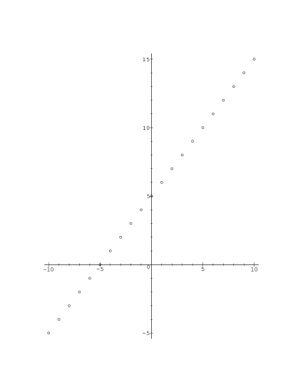
Figure 1: Variable $x$ as a function of $n$ for the lattice (70) $x_{n}=hn+x_{0}$   ($h=1\,,\,x_{0}=5$)

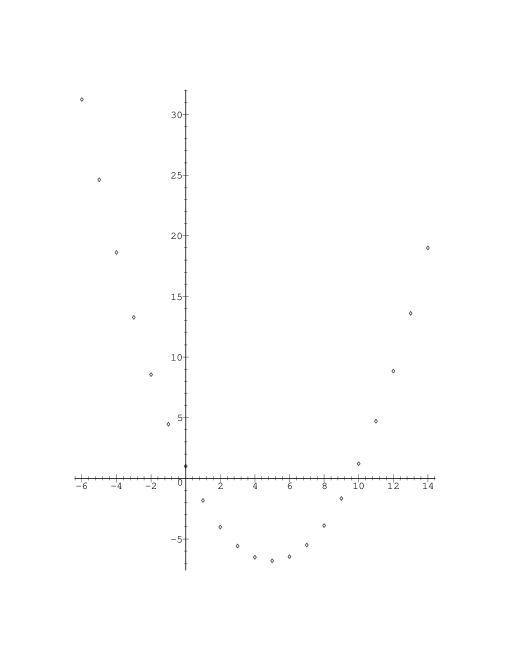
Figure 2: Variable $x$ as a function of $n$ for the lattice (71) $x_{n}=L_{2}n^{2}+L_{1}n+L_{0}$   ($L_{2}=1/\sqrt{10}\,,\,L_{1}=-\pi\,,\,L_{0}=1$)

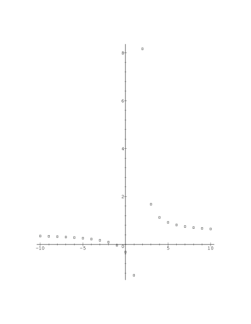
Figure 3: Variable $x$ as a function of $n$ for the lattice (80) $x_{n}=(\alpha n+\beta)(\gamma n+\delta)^{-1}$   ($\alpha=\sqrt{2}$ , $\beta=-\sqrt{3}$ , $\gamma=3$, $\delta=-\sqrt{3}\pi$)

4 Examples for differential-difference equations

In this section we shall need the complete formalism of Section 2, in particular the vector field prolongation (14),…,(17).

4.1 Symmetries of the discrete Volterra equation

The discrete Volterra equation [17] on a uniform lattice is represented by the two equations

$$E \equiv u_{t}+u\,\frac{u_{+}-u_{-}}{x_{+}-x_{-}}=0,$$ (82)

$$\Omega \equiv x_{+}-2x+x_{-}=0,$$ (83)

where $t$ is a continuous variable, $u=u(x,t)$ and $u_{t}=\partial u/\partial t$. The Volterra equation is integrable [17] but we make no use of that here.

The invariance condition for the lattice (83) is

$$\xi(2x-x_{-},t,u_{+})-2\xi(x,t,u)+\xi(x_{-},t,u_{-})=0\,.$$ (84)

Contrary to the cases in Section 3, the values $u_{+},\,u$ and $u_{-}$ in eq.(84) are independent, since the equation $E=0$ involves $u_{t}$ (in addition to $u_{+},\,u$ and $u_{-}$). Differentiating eq.(84) with respect to e.g. $u$ we obtain $\xi_{u}=0$. Differentiating with respect to $x_{-}$ and then $x$, we obtain $\xi_{x_{+}x_{+}}(x_{+},t)=0$. The function $\xi(x,t,u)$ hence reduces to

$$\xi=a(t)x+b(t)$$ (85)

with $a(t)$ and $b(t)$ so far arbitrary functions of $t$.

Invariance of the equation (82) implies:

$$\phi^{t}+\phi\frac{u_{+}-u_{-}}{x_{+}-x_{-}}+\frac{u}{x_{+}-x}(\phi^{(+)}-\phi^{(-)})-\frac{u(u_{+}-u_{-})}{(x_{+}-x_{-})^{2}}(\xi^{(+)}-\xi^{(-)})\left|{}_{E=\Omega=0}\right.=0\,.$$ (86)

The coefficients in the prolongation satisfy

$$\phi^{t} = \phi_{t}+(\phi_{u}-\tau_{t})u_{t}-\xi_{t}u_{x}-\xi_{u}u_{t}u_{x}-\tau_{u}u_{t}^{2}$$ (87)

$$\phi^{(\pm)} = \phi\left(x_{\pm},t,u(x_{\pm},t)\right).$$ (88)

We substitute (85), (87) and (88) into eq.(86) and eliminate $u_{t}(x,t)$ and $x_{+}$ using the equations (82) and (83). The only term involving $u_{x}$ is in $\phi^{t}$. Its coefficient $\xi_{t}$ must vanish and we find $\dot{a}=\dot{b}=0$ in the expression (85).

The remaining determining equation is

$$\begin{array}[]{l}\left\{\phi_{t}+[\phi-u(\phi_{u}-\tau_{t}-au)]\frac{u_{+}-u_{-}}{x_{+}-x_{-}}\right.\\[8.61108pt] +\left.\frac{u}{x_{+}-x_{-}}\left[\phi(x_{+},t,u(x_{+},t))-\phi(x_{-},t,u(x_{-},t))\right]\right\}_{x_{+}=2x-x_{-}}=0\,.\end{array}$$ (89)

We differentiate twice with respect to $u_{+}$ and obtain $\phi_{u_{+}u_{+}}=0$, so that we have $\phi(x,t,u)=\phi_{1}(x,t)u+\phi_{0}(x,t)$. Substituing back into eq.(89) we obtain the final result, namely

$$\xi=ax+b\ \ ,\ \ \tau=c_{1}t+c_{2}\ \ ,\ \ \phi=(a-c_{1})u\,.$$ (90)

Thus, the difference scheme (82), (83) which is the usual Volterra equation, is invariant under a $4$-dimensional group of Lie point transformations. The symmetry algebra is spanned by

$$\hat{P}_{0}=\partial_{t}\ \ ,\ \ \hat{P}_{1}=\partial_{x}\ \ ,\ \ \hat{D}_{0}=t\partial{t}-u\partial_{u}\ \ ,\ \ \hat{D}_{1}=x\partial{x}+u\partial_{u}$$ (91)

(two translations and two dilatations).

The continuous limit of the system (82), (83) is the Euler equation in $1+1$ dimensions

$$u_{t}+uu_{x}=0\,.$$ (92)

Its symmetry group is infinite-dimensional and can be obtained by standard techniques [3, …,8] (though we have not found it given explicitely in the literature). Its symmetry algebra is spanned by

$$\begin{array}[]{c}\hat{X}(\xi)=\xi(z,u)\partial_{x}\ \ ,\ \ \hat{T}(\tau)=\tau(z,t,u)\left(\partial_{t}+u\partial_{x}\right)\\[8.61108pt] \hat{F}(\phi)=\phi(z,u)\left(t\partial_{x}+\partial_{u}\right)\ \ ,\ \ z=x-ut\end{array}$$ (93)

where $\xi,\,\tau$ and $\phi$ are arbitrary functions of their arguments.

The Volterra equation (82) is certainly not a ‘symmetry preserving’ discretization of the Euler equation (92) on a uniform lattice. It only preserves the four-dimensional subalgebra (91) of the infinite-dimensional symmetry algebra (93). Let us mention here that eq.(82) is well known to be a bad numerical scheme for eq.(92).

4.2 A general nearest neighbour interaction equation

Let us consider the difference scheme

$$E \equiv u_{tt}-F(t,x_{+},x,x_{-},u_{+},u,u_{-})=0\,,$$ (94)

$$\Omega \equiv x_{+}-2x+x_{-}=0\,,$$ (95)

where $F$ is an arbitrary smooth function satisfying

$$(F_{u_{+}},F_{u_{-}})\not\equiv(0,0)\,.$$ (96)

A symmetry analysis of a similar class of equations was recently performed for a fixed (non transformable) regular lattice [12]. More specifically, the assumption was $x_{n}=n,\,n\in Z$.

The prolongation formula for the vector field (13) is (14),…,(17). Applying it to eq.(95) we obtain that $\xi$ has the form (85), just as for the Volterra equation. Applying the prolongation to the eq.(94) we obtain

$$\phi^{tt}-\tau F_{t}-(ax+b)F_{x}-(ax_{+}+b)F_{x_{+}}-(ax_{-}+b)F_{x_{-}}-\phi F_{u}-\phi^{(+)}F_{u_{+}}-\phi^{(-)}F_{u_{-}}\left|{}_{E=\Omega=0}\right.=0\,.$$ (97)

We substitute the expression for $\phi^{tt},\,\phi^{(+)}$ and $\phi^{(-)}$ and set the coefficients of $u_{t}^{3}$, $u_{t}^{2}$, $u_{t}^{2}u_{x}$, $u_{t}u_{xt}$, $u_{xt}$, $u_{t}$ equal to zero, after eliminating $u_{tt}$ and $x_{+}$, using equations (94), (95). The result is that for any interaction $F$ satisfying condition (96), we have

$$\tau=\tau(t)\ \ ,\ \ \xi=ax+b\ \ ,\ \ \phi=\left[\frac{\dot{\tau}}{2}+\alpha(x)\right]u+B(x,t)\,.$$ (98)

The as yet unspecified functions $\tau(t),\,\alpha(x),\,B(x,t)$ and constants $a,\,b$ satisfy a remaining determining equation, namely

$$\begin{array}[]{l}\left\{\frac{1}{2}\tau_{ttt}u+B_{tt}-(\frac{3}{2}\tau_{t}-\alpha)F+\tau F_{t}-(ax+b)F_{x}-(ax_{+}+b)F_{x_{+}}\right.\\[8.61108pt] -(ax_{-}+b)F_{x_{-}}-\left[(\frac{1}{2}\tau_{t}+\alpha(x))u+B\right]F_{u}-\left[(\frac{1}{2}\tau_{t}+\alpha(x_{+}))u_{+}+B(x_{+},t)\right]F_{u_{+}}\\[8.61108pt] \left.-\left[(\frac{1}{2}\tau_{t}+\alpha(x_{-}))u_{-}+B(x_{-},t)\right]F_{u_{-}}\right\}_{x_{+}=2x-x_{-}}=0\,.\end{array}$$ (99)

The results (98), (99) agree with those of Ref.[12], but are more general. The reason for the increase in generality is that here the lattice is not fixed a priori and hence the vector field (13) contains a term proportional to $\partial_{x}$.

To proceed further, we restrict the interaction $F$ to have a specific form.

4.3 Equation with $F=(x_{+}-x)^{6}(u_{+}-2u+u_{-})^{-3}$

Let us consider a special case of the system (94), (95), namely

$$u_{tt}=\frac{(x_{+}-x)^{6}}{(u_{+}-2u+u_{-})^{3}},$$ (100)

$$x_{+}-2x+x_{-}=0.$$ (101)

We substitute $F$ of eq.(100) into the determining equation (99) and clear the denominator. The dependence on $u,\,u_{+}$ and $u_{-}$ is explicit and we obtain

$$\begin{array}[]{l}\tau_{ttt}=0\ \ ,\ \ B_{tt}=0\ \ ,\ \ B(x_{+},t)-2B(x,t)+B(x_{-},t)=0,\\[8.61108pt] \alpha(x)(x_{+}-x)+6(ax+b)-6(ax_{+}+b)+3\alpha(x_{+})(x_{+}-x)=0\,.\end{array}$$ (102)

Analysing the system (102) in the usual manner, we obtain a 9-dimensional Lie algebra with basis

$$\begin{array}[]{c}\hat{P}_{0}=\partial_{t}\ ,\ \hat{P}_{1}=\partial_{x}\ ,\ \hat{D}_{1}=2t\partial_{t}+u\partial{u}\ ,\ \hat{D}_{2}=2x\partial_{x}+3u\partial{u},\\[8.61108pt] \hat{C}=t^{2}\partial_{t}+tu\partial{u}\ ,\ \hat{W}_{1}=\partial{u}\ ,\ \hat{W}_{2}=t\partial{u}\ ,\ \hat{W}_{3}=x\partial{u}\ ,\ \hat{W}_{4}=tx\partial{u}\,.\end{array}$$ (103)

A related system was studied earlier [12], namely

$$\ddot{u}_{n}(t)=\left[(\gamma_{n}-\gamma_{n-1})u_{n+1}+(\gamma_{n+1}-\gamma_{n-1})u_{n}+(\gamma_{n-1}-\gamma_{n})u_{n+1}\right]^{-3},$$ (104)

where $\gamma_{n}$ is any function of $n$, satisfying $\gamma_{n+1}\not\equiv\gamma_{n}$. If we take $\gamma_{n}=n$ in eq.(104) and $x=n$ in (100), (101) the two systems coincide. The symmetry algebra found in Ref.[12] is the subalgebra $\{\hat{P}_{0}\,,\,\hat{D}_{1}\,,\,\hat{C}\,,\,\hat{W}_{1}\,,\,\hat{W}_{2}\,,\,\hat{W}_{3}\,,\,\hat{W}_{4}\}$ of the algebra (103). The elements $\hat{P}_{1}$ and $\hat{D}_{2}$ are absent, since the lattice is fixed. Shifts $n^{\prime}=n+N$ are allowed, but are not infinitesimal.

The system (100), (101) has a continuous limit

$$u_{tt}=\frac{1}{u_{xx}^{3}}\,.$$ (105)

The symmetry algebra of eq.(105) coincides with (103), i.e. the system (100), (101) is a symmetry preserving discretization of eq.(105). We emphasize that eq.(100) was obtained as part of a classification of difference equations [12], not in any connection with the PDE (105).

4.4 Equation without a continuous limit

Let us now consider another special case of the system (94), (95), namely

$$u_{tt}=\frac{1}{(u_{+}-2u+u_{-})^{3}} x_{+}-2x+x_{-}=0\,.$$ , (106)

Substituing for $F$ into eq.(99) and proceeding as in Section 4.3. we again obtain a 9-dimensional symmetry algebra. It differs from that given in eq.(103) only in that $D_{2}$ is replaced by $\tilde{D}_{2}=x\partial{x}$. For $h=x_{+}-x$ satisfying $h\rightarrow 0$ we find $u_{tt}$ finite, but $(u_{+}-2u+u_{-})^{-3}\rightarrow\infty$, so the limit $h\rightarrow 0$ does not exist.

5 Conclusions

The main questions to be addressed in a program aiming at using Lie group theory to solve difference equations are: (i) How does one define the symmetries? (ii) How does one calculate the symmetries? (iii) What does one do with the symmetries?

In this article we define the symmetries as in eq.(9), that is we consider only Lie point transformations that act simultaneously in a difference equation (1) and lattice equation (2). The fact that the lattice also transforms is in the spirit of Dorodnitsyn’s approach to discretizing differential equations. In most symmetry studies of difference equations [9, …, 26] the lattice is fixed and nontransformable, e.g. given by the equation $x=n,\,n\in Z$. For nontransforming lattices we need to go beyond point symmetries to catch transformations of interest[17].

Once the class of symmetries that we wish to consider is defined, the matter of calculating them becomes purely technical. We proposed an algorithm for calculating symmetries in Section 2 (see eq. (13),…,(18)) and applied it in Section 3 and 4. Symmetry algorithms for fixed lattices were presented elsewhere [10, -, 14].

Equations (100) and (104) provide good examples of different approaches. The symmetry algebra (103) of the system (100), (101) happens to coincide with the symmetry algebra of the continuous limit (105). The symmetry algebra of the related equation (104) was calculated elsewhere [12]. It is a 7-dimensional subalgebra of the algebra (103), obtained by dropping $\hat{P}_{1}$ and $\hat{D}_{2}$. It was obtained by the ‘intrinsic method’ [11]. The symmetry algebra of eq.(104) can also be obtained from that of the system (100), (101) by taking a specific solution $x=n$ of eq.(101) and reducing the algebra (103) to the one that preserves this solution.

As far as applications of symmetries are concerned, they are the same for differential equations and difference ones, in particular, symmetry reduction.

First, consider translationally invariant solutions, i.e. solutions invariant under the subgroup generated by $\hat{X}=\hat{P}_{0}-v\hat{P}_{1}$ with $v$ constant and $\hat{P}_{0},\,\hat{P}_{1}$ as in eq.(103). We find that the solution, the differential-difference equations (D$\Delta$E) (100), (101) and the PDE (106) reduce to

$$u(x,t)=G(\eta)\ \ ,\ \ \eta=x+vt$$ (107)

$$v^{2}G_{\eta\eta}[G(\eta+h)-2G(\eta)+G(\eta-h)]^{3}=h^{6}$$ (108)

$$v^{2}G_{\eta\eta}^{4}=1$$ (109)

respectively. Surprisingly, the difference equation (108) and the ODE (109) have exactly the same solution for all values of the spacing $h$, namely

$$G=\pm\frac{1}{2\sqrt{v}}\eta^{2}+A\eta+B\ \ ,\ \ v\not\equiv 0$$ (110)

where $A$ and $B$ are integration constants. Thus, the system (100), (101) is not only a symmetry preserving discretization. It also preserves translationally invariant solutions.

As a second example, consider solutions invariant under dilations generated by $\hat{D}_{1}$ of eq.(103).The reduction formula, reduced D$\Delta$E and reduced PDE are

$$u(x,t)=t^{1/2}G(x)$$ (111)

$$G(x)\,[G(x+h)-2G(x)+G(x-h)]^{3}=-4h^{6}$$ (112)

$$G\,G_{xx}^{3}=-4$$ (113)

respectively. A particular solution of eq.(113) is $G(x)=4(-3)^{-3/4}(x-x_{0})^{3/2}$. This is not an exact solution of eq.(112), but the solution of (112) and (113) coincide to order $h^{2}$, rather than just $h$.

As a final example of symmetry reduction, consider the subgroup corresponding to $\hat{D}_{2}-3\hat{D}_{1}$ of eq.(103). The reduction formulas are

$$u(x,t)=G(\eta)\ \ ,\ \ \eta=x^{3}t$$ (114)

$$G_{\eta\eta}=\frac{(\eta_{+}^{1/3}-\eta^{1/3})^{6}}{\eta^{2}[G(\eta_{+})-2G(\eta)+G(\eta_{-})]^{3}}\ \ ,\ \ \eta_{+}^{1/3}-2\eta^{1/3}+\eta_{-}^{1/3}=0$$ (115)

$$27\eta^{3}G_{\eta\eta}[3\eta G_{\eta\eta}+2G_{\eta}]^{3}=1$$ (116)

While we are not able to solve the ODE (116), nor the difference scheme (115), we see that in both cases we get a reduction of the number of independent variables. We mention that this last reduction would not be obtained on a fixed lattice.

Let us sum up the situation with this particular approach to symmetries of difference equations.

1. Lie point symmetries acting simultaneously on given equations and lattices can be calculated using the reasonably simple algorithm presented in this article.

2. Symmetries can be used to perform symmetry reduction for D$\Delta$E.

Work is in progress on other applications of symmetries of discrete equations, in particular solving ordinary difference equations.

References

• [1] S. Lie, Klassifikation und Integration von Gewohnlichen Differentialgleichungen zwischen $x,y$ die eine Gruppe von Transformationen gestatten, Math. Ann. 32, 213 (1888)
• [2] S. Lie, Theorie der Transformationgruppen (B.G. Teubner, Leipzig, 1888, 1890, 1893)
• [3] P.J. Olver, Applications of Lie Groups to Differential Equations (Springer, New York, 1993)
• [4] N.H. Ibragimov, Transformation Groups Applied to Mathematical Physics (Reidel, Boston, 1985)
• [5] L.V. Ovsiannikov, Group Analysis of Differential Equations (Academic, New York, 1982)
• [6] G.W. Bluman and S. Kumei, Symmetries and Differential Equations (Springer, Berlin, 1989)
• [7] G. Gaeta, Nonlinear Symmetries and Nonlinear Equations (Kluwer, Dordrecht, 1994)
• [8] P. Winternitz, Group theory and exact solutions of nonlinear partial differential equations, In Integrable Systems, Quantum Groups and Quantum Field Theories, 429–495, Kluwer, Dordrecht, 1993.
• [9] S. Maeda, Canonical structure and symmetries for discrete systems, Math. Japan 25, 405 (1980)
• [10] D. Levi and P. Winternitz, Continuous symmetries of discrete equations, Phys. Lett. A 152, 335 (1991)
• [11] D. Levi and P. Winternitz, Symmetries and conditional symmetries of differential-difference equations, J. Math. Phys. 34, 3713 (1993)
• [12] D. Levi and P. Winternitz, Symmetries of discrete dynamical systems, J. Math. Phys. 37, 5551 (1996)
• [13] D. Levi, L. Vinet, and P. Winternitz, Lie group formalism for difference equations, J. Phys. A: Math. Gen. 30, 663 (1997)
• [14] R. Hernandez Heredero, D. Levi, and P. Winternitz, Symmetries of the discrete Burgers equation, J. Phys. A Math. Gen. 32, 2685 (1999)
• [15] D. Gomez-Ullate, S. Lafortune, and P. Winternitz, Symmetries of discrete dynamical systems involving two species, J. Math. Phys. 40, 2782 (1999)
• [16] S. Lafortune, L. Martina and P. Winternitz, Point symmetries of generalized Toda field theories, J. Phys. A: Math. Gen. 33, 2419 (2000)
• [17] R. Hernandez Heredero, D. Levi, M.A. Rodriguez and P. Winternitz P, Lie algebra contractions and symmetries of the Toda hierarchy, J. Phys. A: Math. Gen. (in press)
• [18] D. Levi and R. Yamilov, Conditions for the existence of higher symmetries of evolutionary equations on the lattice, J. Math. Phys. 38, 6648 (1997)
• [19] D. Levi and R. Yamilov, Non-point integrable symmetries for equations on the lattice, J. Phys. A: Math. Gen. (in press)
• [20] D. Levi, M.A. Rodriguez, Symmetry group of partial differential equations and of differential-difference equations: the Toda lattice vs the Korteweg-de Vries equations, J. Phys. A: Math. Gen. 25, 975 (1992)
• [21] D. Levi, R. Yamilov, Dilatation symmetries and equations on the lattice, J. Phys. A: Math. Gen. 32, 8317 (1999)
• [22] D. Levi, M.A. Rodriguez, Lie symmetries for integrable equations on the lattice, J. Phys. A: Math. Gen. 32, 8303 (1999)
• [23] R. Floreanini, J. Negro, L.M. Nieto and L. Vinet, Symmetries of the heat equation on a lattice, Lett. Math. Phys. 36, 351 (1996)
• [24] R. Floreanini and L. Vinet, Lie symmetries of finite-difference equations, J. Math. Phys. 36, 7024 (1995)
• [25] G.R.W. Quispel, H.W. Capel, and R. Sahadevan, Continuous symmetries of difference equations; the Kac-van Moerbeke equation and Painleve reduction, Phys. Lett. A 170, 379 (1992)
• [26] G.R.W. Quispel and R. Sahadevan, Lie symmetries and integration of difference equations, Phys. Lett. A 184, 64 (1993)
• [27] V.A. Dorodnitsyn, Transformation groups in a space of difference variables, in VINITI Acad. Sci. USSR, Itogi Nauki i Techniki, 34, 149–190 (1989), (in Russian), see English translation in J. Sov. Math. 55, 1490 (1991)
• [28] W.F. Ames, R.L. Anderson, V.A. Dorodnitsyn, E.V. Ferapontov, R.K. Gazizov, N.H. Ibragimov and S.R. Svirshchevskii, CRC Hand-book of Lie Group Analysis of Differential Equations, ed. by N.Ibragimov, Volume I: Symmetries, Exact Solutions and Conservation Laws, CRC Press, 1994.
• [29] V.A. Dorodnitsyn, Finite-difference models entirely inheriting continuous symmetry of original differential equations. Int. J. Mod. Phys. C, (Phys. Comp.), 5, 723 (1994)
• [30] V. Dorodnitsyn, Continuous symmetries of finite-difference evolution equations and grids, in Symmetries and Integrability of Difference Equations, CRM Proceedings and Lecture Notes, Vol. 9, AMS, Providence, R.I., 103–112, 1996, Ed. by D.Levi, L.Vinet, and P.Winternitz, see also V.Dorodnitsyn, Invariant discrete model for the Korteweg-de Vries equation, Preprint CRM-2187, Montreal, 1994.
• [31] M. Bakirova, V. Dorodnitsyn, and R. Kozlov, Invariant difference schemes for heat transfer equations with a source, J. Phys. A: Math.Gen., 30, 8139 (1997) see also V. Dorodnitsyn, R. Kozlov, The complete set of symmetry preserving discrete versions of a heat transfer equation with a source, Preprint of NTNU, NUMERICS NO. 4/1997, Trondheim, Norway, 1997.
• [32] V. Dorodnitsyn, Finite-difference models entirely inheriting symmetry of original differential equations Modern Group Analysis: Advanced Analytical and Computational Methods in Mathematical Physics (Kluwer Academic Publishers), 191, 1993.
• [33] V.A. Dorodnitsyn, Finite-difference analog of the Noether theorem, Dokl. Akad. Nauk, 328, 678, (1993) (in Russian). V. Dorodnitsyn, Noether-type theorems for difference equation, IHES/M/98/27, Bures-sur-Yvette, 1998.
• [34] V. Dorodnitsyn and P. Winternitz, Lie point symmetry preserving discretizations for variable coefficient Korteweg - de Vries equations, CRM-2607, Universite de Montreal, 1999 ; to appear in Nonlinear Dynamics, Kluwer Academic Publisher, 1999.
• [35] V. Dorodnitsyn, R. Kozlov and P. Winternitz P, Lie group classification of second order ordinary difference equations, J. Math. Phys. 41, 480 (2000)
• [36] D. Levi, L. Vinet, and P. Winternitz (editors), Symmetries and Integrability of Difference Equations, CRM Proceedings and Lecture Notes vol. 9, (AMS, Providence, R.I., 1996)
• [37] P.A. Clarkson and F.W. Nijhoff (editors), Symmetries and Integrability of Difference equations (Cambridge University Press, Cambridge, UK, 1999)