Abstract

We present analytical investigations of a multiplicative stochastic process that models a simple investor dynamics in a random environment. The dynamics of the investor’s budget, $x(t)$, depends on the stochasticity of the return on investment, $r(t)$, for which different model assumptions are discussed. The fat-tail distribution of the budget is investigated and compared with theoretical predictions. We are mainly interested in the most probable value $x_{\mathrm{mp}}$ of the budget that reaches a constant value over time. Based on an analytical investigation of the dynamics, we are able to predict $x_{\mathrm{mp}}^{\mathrm{stat}}$. We find a scaling law that relates the most probable value to the characteristic parameters describing the stochastic process. Our analytical results are confirmed by stochastic computer simulations that show a very good agreement with the predictions.

Keywords: multiplicative stochastic processes; scaling laws; investment dynamics; PACS: 05.40.-a, 05.10.Gg

1 Introduction

Multiplicative stochastic processes denote type of dynamics where a variable $x(t)$ changes its value in time due to a stochastic term $\lambda(t)$:

$$x(t+1)=\lambda(t)\,x(t)$$ (1)

$\lambda(t)$ may describe different stochastic processes, such as Gaussian white noise, uniform random distributions, GARCH or ARCH processes, which are explained later in this paper. Despite its great simplicity, the dynamics of eqn. (1) gained much attention in different fields of applications. It was, for example, used already in 1931 by Gibrat to describe the annual growth of companies – an idea extended in different works by economists [42, 10] and econophysicists [1]. Several theoretical aspects of stochastic processes with multiplicative noise have been focus of recent research in physics [31, 20, 44, 41, 40]. Moreover, by taking into account additional couplings between these processes, the approach has been extended towards a generalized Lotka-Volterra model [22, 39] which is referred to later in this paper.

The importance of multiplicative stochastic processes was also reflected by several mathematical investigations [46, 12, 13]. In the so-called Kesten process [16] – from which we depart in this paper – the dynamics of eqn. (1) was extended by a second additive stochastic term $a(t)$ independent of $\lambda(t)$

$$x(t+1)=\lambda(t)\,x(t)+a(t)$$ (2)

This extension has the nice feature that the stochastic process is repelled from zero, provided some constraints on $a(t)$ are satisfied. We will come back to this later in our paper. At this point, we rather want to provide some arguments why we became interested in this topic and why we think that this is relevant.

Our investigations started with the question of how much “intelligence” is needed for an agent to survive in a noisy environment (see also [9]). The example at hand is explained in Sect. 2.1: agents with a personal budget, $x(t)$, participate in a simple investment scenario and face a return on their investment, $r(t)$. Given some uncertainty of $r(t)$, they have the choice to adjust individually the portion of the budget they wish to invest, $q(t)$, which can be called their risk propensity. The strategy to choose $q(t)$ may of course depend on whether the agents are able to obtain some information about the expected return on investment, $r(t)$. Here, different levels of internal complexity, or “intelligence”, of agents come into play, namely their capability to observe and to store a history of previous returns $r(t-\tau)$, to calculate different measures from such a time series (such as trends, moving least squares, etc.), to detect or to forecast certain periodicities in the signal received (such as cycles in the market) [27, 26]. At this point, a wealth of different models, assumptions, suggestions, speculations etc. about the agent’s behavior comes into play from various fields (financial theory [24, 19, 9, 30], economics [21, 45, 5, 17, 29, 11], behavioral sciences [43], physics [25, 23, 6], computer sciences [18, 7, 15]). All these rather complex assumtions eventually lead to their specific outcome of the game, and can hardly be compared. So, before embarking on some more refined modeling assumptions about agents behavior, we had to ask ourselves what could be the reference case in this simple investment scenario, to which later all advanced simulations can be compared. In other words: what would be the dynamics of that investment process without all these “intelligent” assumptions? It turns out that this baseline case is exactly given by the dynamics of a multiplicative stochastic process with an additive term as described by eqn. (2). Instead of a rather complex strategy $q(t)$, we simply assume $q_{0}=\mathrm{const.}$ as the reference case, instead of an unknown additional influx $a(t)$, we take a constant, but positive “income” $a$, and instead of specific economic assumptions about market fluctuations we choose $r(t)$ from four different stochastic processes, which are simple, but analytically tractable. This way, in Sect. 2.1 we arrive at the basic dynamics of eqn. (12), which is equivalent to our starting equation (2).

The aim of our paper is (i) to elucidate the dynamics of eqn. (2) for some specific settings of $\lambda(t)$ and $a(t)$ by means of some computer simulations, and (ii) to investigate its stationary properties by means of analytical treatment. This will reveal some scaling between the most probable value of $x(t)$ and the parameters describing the stochastic processes. Before we continue in this direction, we want to shortly summarize some previous theoretical investigations of eqn. (2), in order to refer to it later.

The dynamics of eqn. (2) was treated by Sornette and Cont [41] as

$$\frac{x(t+1)-x(t)}{x(t)}=\frac{a(t)}{x(t)}+\lambda(t)-1$$ (3)

If the finite difference ${\left(x(t+1)-x(t)\right)}/{x(t)}$ is approximated by $(d\log x/dt)$, the following overdamped Langevin equation for $w=\log{x}$ can be obtained:

$$\frac{dw}{dt}=a(t)e^{-w}-\left|\upsilon\right|+\eta(t)$$ (4)

with:

$$\upsilon=\left\langle\lambda\right\rangle-1\simeq\left\langle\log\lambda\right\rangle\;\quad\left\langle\eta^{2}\right\rangle=\left\langle\lambda^{2}\right\rangle-\left\langle\lambda\right\rangle^{2}$$ (5)

The first term on the r.h.s. of eqn. (4) describes an effective repulsion of $x$ from zero, while the second term, $-\left|\upsilon\right|$, describes the drift towards zero. The third term, $\eta(t)$, expresses the stochastic influences resulting from $\lambda(t)$.

Going over from the single stochastic realizations of $\omega(t)$ to the probability density $P(\omega,t)$, it was shown in [41] that the following Fokker-Planck equation can be derived

$$\frac{\partial P(w,t)}{\partial t} = a(t)\,e^{-w}\,P(w,t)-\left(\left\langle\log{\lambda}\right\rangle+a(t)\,e^{-w}\right)\frac{\partial P(w,t)}{\partial w}$$ (6)

$$+\left(\left\langle\log{(\lambda)^{2}}\right\rangle-\left\langle\log{\lambda}\right\rangle^{2}\right)\,\frac{1}{2}\frac{\partial^{2}P(w,t)}{\partial w^{2}}$$

In accordance with eqn. (4), the first term of eqn. (6) describes the decay on $w$, the second term indicates the drift of the process and the third is a diffusion term with the diffusion constant:

$$D=\left\langle(\log{\lambda})^{2}\right\rangle-\left\langle\log{\lambda}\right\rangle^{2}$$ (7)

We recall that without the additive stochastic force, i.e. $a(t)\equiv 0$, eqn. (6) results in a simple Fokker-Planck equation for $x(t)$, related to the stochastic eqn. (1), with the log-normal distribution as limit distribution [31, 41]:

$$P(x(t))=\frac{1}{\sqrt{\pi\,D\,t}}\,\frac{1}{x(t)}\,\exp{\left\{-\frac{1}{D\,t}\big{[}\log{x(t)}-\left\langle\log{\lambda}\right\rangle\,t\big{]}^{2}\right\}}$$ (8)

Considering, however, an additive stochastic force $a(t)\not\equiv 0$, it was already noted in [16] that for large $x$ instead of a log-normal distribution now a power-law distribution results, provided that $\left\langle\log\lambda\right\rangle<0$:

$$P(x)\propto x^{-(1+\mu)}$$ (9)

The exponent $\mu$ satisfies the conditions

$$\left\langle\lambda^{\mu}\right\rangle=1\;;\quad\mu=\frac{2\left|\left\langle\log{\lambda}\right\rangle\right|}{\left\langle(\log{\lambda})^{2}\right\rangle-\left\langle\log{\lambda}\right\rangle^{2}}=\frac{2\left|v\right|}{D}$$ (10)

It was shown [41] that such power-laws result under quite general assumptions about multiplicative stochastic processes with repulsion at the origin which generalizes previous results by [20]. We note that an economically motivated entry/exit dynamics [36, 3, 32] as a boundary condition of the multiplicative stochastic process also leads to power distributions.

In the more general case of eqn. (6), we will in Sect. 3.1 provide a stationary solution for $P(\omega)$ at least for the case of a constant $a$. We will further use this solution to derive a result for the most probable value of the multiplicative stochastic process. In order to test the analytical predictions, we will compare them with stochastic computer simulations, which are described in the following section.

2 Computer simulations for different random environments

2.1 Investment model

Instead of solving the stochastic differential equation (6) numerically, in this section we focus on the individual realizations of the stochastic process as described by eqn. (2). Hence, we have to specify the stochastic processes behind the variables $\lambda(t)$ and $a(t)$, which is done in the following. As it became clear from the previous discussion, the additive stochastic term acts as a repulsion of the dynamics from zero, i.e. without $a(t)$ after some time every stochastic realization of $x(t)$ will reach the value zero, i.e., the exit for the process. So, the meaning of $a(t)$ is simply to keep the dynamics “alive” by preventing it from reaching zero. To simplify the dynamics, instead of a time-dependent value $a(t)$ we simply choose a small, but constant positive value of $a$, which results in the same effect.

For the multiplicative stochastic term the following assumption was made:

$$\lambda(t)=1+r(t)\,q(t)$$ (11)

In order to give the stochastic dynamics of eqs. (2), (11) some interpretation, let us consider the following: $x(t)$ shall represent the budget (wealth, liquidity) of an agent, who intents to invest some portion $0\leq q(t)\leq 1$ of its budget into a market [26, 27]. Depending on the market performance, this investment may result in a loss or a gain. Hence, there exists a return on investment, RoI, $r(t)$, which is either positive or negative. It should be noted that the RoI has to satisfy $r(t)>-1$ as a lower boundary, as investors can never loose more than what they have invested. Because there is no limit for potential profits, in principle there is no upper boundary for $r(t)$.

In a real investment scenario, the RoI can be determined from a time series of a real market that is influenced by several thousands bids and asks. This would involve to model the market dynamics explicitely. In the spirit of other investigations in economics and econophysics [1] we have chosen instead to model the market return $r(t)$ by means of different stochastic processes, i.e. to keep its dynamics independent of the investment of the agent. Further, we have bound the RoI to values between -1 and +1. The upper boundary was chosen to obtain a mean of zero for $r(t)$, which allows to better understand the basic dynamics. The following distributions for $r(t)$ are discussed:

1. $B\{-1,1\}$, a binary stochastic switch between only two states, -1 and +1

2. $U(-1,1)$, a uniform distribution, where every possible value between -1 and +1 has the same probability to be chosen

3. $N(0,0.1)$, a normal distribution with mean $0$ and standard deviation 0.1, i.e. values close to the mean are more likely to be picked

4. ARCH(1), a distribution, where possible values between -1 and +1 are chosen by considering some correlations between times $t$ and $t-1$ (autoregressive conditional heteroskedasticity) [2, 8].

These stochastic processes were not chosen in the first place because they capture real economic processes e.g. on financial markets, but because they later allow for analytical calculations of some properties of the probability distributions, as shown in Sect. 3.2. However, we note that the four types cover different degrees of complexity in the stochastic process, as their spectrum of values (discrete, continuous) and their range of values (rather broad for the uniform distribution, but narrowed and centered for the normal distribution) vary and even correlations between different time steps are taken into account (ARCH(1)).

The investment dynamics is then described by the multiplicative stochastic process

$$x(t+1)=x(t)\,\left[1+r(t)\,q(t)\right]+a$$ (12)

where the positive constant $a$ prevents the investor from going bankrupt.

The challenge for an agent in this very simple investment model is then to adjust its portion of the budget to be invested, $q(t)$, given some (observed) market returns $r(t)$. Low values of $q$ refer to a risk averse investment strategies, while higher values may be more risky, but also more rewarding with respect to the budget. In [27] we have discussed different scenarios for agents to adjust their risk propensity, $q(t)$. In this paper we focus more on the stochastic dynamics and therefore just choose $q(t)=q_{0}$, which is a small but constant value. This can serve as a reference case for more complex investment strategies [27].

At this point, we wish to note that the dynamics proposed in eqn. (12) is much simpler than the comparable starting equation in the generalized Lotka-Volterra model [22, 39] mentioned in Sect. 1,

$$x_{i}(t+1)=x_{i}(t)\,\left[1+\lambda(t)\right]+a\bar{x}(t)-Cx_{i}(t)$$ (13)

which assumes additional couplings between different individual stochastic processes, $x_{i}(t)$. Instead of a small, but constant income $a$ the term $a\bar{x}(t)$ considers a global coupling via the mean budget $\bar{x}(t)$ of all agents (which may be related to general publicly funded services). Moreover, the third term $Cx_{i}(t)$ describes direct interactions between different agents, as $C$ is a function dependent on other $x_{j}$. These may account for competition for limited resources and saturation effects in the dynamics. Even if, after some approximations discussed in [22], these additional influences may be small, they still affect the general solutions for the underlying probability distributions as we will discuss in Sect. 3.1. If we recast the differences between eqs. (12), (13) using the general framework of multiplicative processes [33]

$$\Delta x(t)=\eta(t)G[x(t)]+F[x(t)]$$ (14)

where $\eta(t)$ is a stochastic variable, then we have for our model, eqn. (12) $G(x)=x$ and $F(x)=a$, whereas for eqn. (13) $G(x)=x$ and $F(x)=a(1-x)$ results [22]. This will eventually affect the specific exponents of the stationary probability distributions, $P_{s}(x)$.

2.2 Simulation results

Here, we present stochastic computer simulations of eqn. (12) for different distributions of $r(t)$ as described in the previous section. Initially, $x(0)=10$ holds for the agent’s budget, $q_{0}$ and $a$ are kept constant during each simulation. The distributions were realized using 10’000 agents. In the case of the time evolution of the most probable value $x_{mp}$, the plotted values were calculated averaging over the $x_{mp}$ obtained for distributions resulting from 10 different realizations of the simulation.

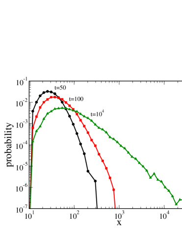
Figure 1: Investor’s budget probability distribution $P(x,t)$ for different time steps, assuming $x(0)=10$ and $r(t)\in B\{-1,1\}$, $q_{0}=0.1$ and $a=0.5$. The probability was estimated from $N=10^{4}$ runs.

Figure 1 shows the distribution of the investor’s budget at different time steps. Starting from the delta distribution at $x(0)=10$, the distribution disperses over time until it reaches a stationary state. The number of time steps needed to reach this stationary state depends on the initial conditions, the distribution of $r(t)$ and the additive constant $a$. For the conditions in Figure 1, this takes about $10^{4}$ iterations.

One can clearly see that the stationary distribution is characterized by a fat tail described by a power-law distribution, as shown in Figures 2. This is in accordance with previous investigations [40, 20] and was already discussed in Sect. 1. We have determined the scaling exponent $\mu$ of the power law, eqn. 9, from the simulation data for different stochastic processes and will later compare it with our analytical investigations.

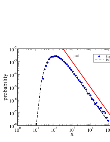
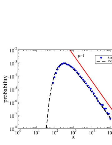
Figure 2: Investor’s budget stationary probability distribution $P_{s}(x)$ (estimated from frequencies after $t=10^{4}$): (left) Binary stochastic return distribution $r(t)=B\{-1,1\}$. (right) Uniform stochastic return distributions $r(t)=U(-1,1)$. In both cases, $x(0)=10$, $q(t)=0.1$ and $a=1$. Data is binned in logarithmic intervals of the same size. The dashed lines show the theoretical prediction of these curves by Eqn. (21), derived later.

In the following, we are more interested in the clear maximum of the stationary distribution which gives the most probable value, $x_{\mathrm{mp}}$. Figure 3 (right) shows the evolution of $x_{\mathrm{mp}}$ over time for three different additive terms. The most probable value increases with time until a balanced state is reached, where the dissipation described by the negative drift towards zero and the constant influx $a$ compensate on average. It can be noticed that the standard deviation of $x_{\mathrm{mp}}$ increases with $a$. Larger $a$ lead to larger values for the budgets, this in turn leads to an amplification of the fluctuations due to the multiplicative nature of the process. Figure 3 shows the evolution of $x_{\mathrm{mp}}$ for three different values of the risk propensity $q_{0}$. Obviously, the larger $q$, the smaller $x_{\mathrm{mp}}$.

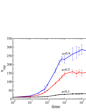
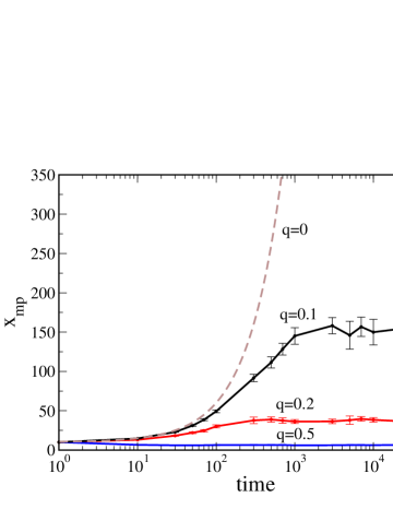
Figure 3: Most probable budget value vs. time: (left) for $q=0.1$ and 3 different additive constants $a$, (right) for $a=0.5$ and 3 different constant risk propensities $q_{0}$. Other parameters and settings as in Figure 2(right).

Figure 3 suggest that there is a scaling between the most probable value $x_{\mathrm{mp}}$ and the parameters characterizing the stochastic dynamics, eqn. (12), namely $q_{0}$ and $a$. This scaling is investigated numerically in the following and will later be confirmed by analytical investigations. Figures 4, 5 show $\left\langle x_{\mathrm{mp}}\right\rangle$ at a fixed time, $t=10^{4}$, for the four different realizations of the stochastic process, $r(t)$, discussed in Sect. 2.1. In all four cases, the results, plotted against the variable $a/q_{0}^{2}$ clearly show a straight line, which allows for the scaling:

$$x_{\mathrm{mp}}=c\cdot\frac{a}{q_{0}^{2}}$$ (15)

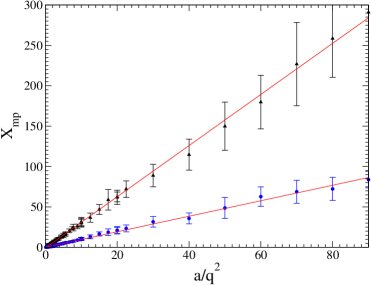
Figure 4: Most probable budget value vs. scaled variable $a/q_{0}^{2}$ for the binary stochastic process $r(t)\in\{-1,1\}$ (o) and for the uniform stochastic process $r(t)\in U(-1,1)$ ($\triangle$). Each set was plotted by varying $a$ and $q_{0}$ over the range of $[0.1,0.9]$ in $0.1$ increments, giving a total of 81 data points per combination, , averaged over 100’000 Monte-Carlo simulations and 10 runs. The value of the slope found for the numerical simulations is for the binary stochastic process $c=0.961\pm 0.006$ and the uniform stochastic process $c=3.149\pm 0.014$

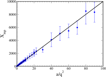
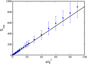
Figure 5: Most probable budget value vs. scaled variable $a/q_{0}^{2}$: (left) for the normal distributed stochastic process $r(t)\in N(0,0.1)$. The value found for the slope of the numerical simulations in this process was: $c=102.17\pm 0.701$, (right) for the ARCH(1) process ($\alpha_{0}=\alpha_{1}=0.1$), with a slope of $c=9.089\pm 0.029$

By means of analytical investigations of the stochastic multiplicative dynamics, we now want to confirm the findings of the numerical experiments.

3 Analytical investigations

3.1 Stationary state

In order to derive the observed scaling law, eqn. (15), we start with the Fokker-Planck eqn. (6). Using the approximation of a constant value of $a$ and the notation of eqn. (7) for the diffusion constant $D$, we find for the stationary solution of eqn. (6):

$$0=-\partial_{w}\left[\left(\left\langle\log\lambda\right\rangle+a\,e^{-w}\right)P_{s}(w)-\frac{D}{2}\partial_{w}P_{s}(w)\right]$$ (16)

This results in the stationary solution:

$$P_{s}(w)=\mathcal{N}\exp\left(\frac{2\left\langle\log\lambda\right\rangle\,w-2a\,e^{-w}}{D}\right)$$ (17)

with normalisation $\mathcal{N}$. Using $w=\log x$, the corresponding stationary probability distribution $P_{s}(x)$ is recovered by the chain rule:

$$P_{s}(x)=P_{s}\left(w(x)\right)\,\frac{dw}{dx}=\mathcal{N}\,x^{\frac{2\left\langle\log\lambda\right\rangle}{D}-1}\,\exp\left(-\frac{2a}{D\,x}\right).$$ (18)

The normalization is explicitely calculated via:

$$1\stackrel{{\scriptstyle!}}{{=}}\mathcal{N}\int_{0}^{\infty}x^{\frac{2\left\langle\log\lambda\right\rangle}{D}-1}\,\exp\left(-\frac{2a}{D\,x}\right)\,dx=\mathcal{N}\left(\frac{D}{2a}\right)^{-\frac{2\left\langle\log\lambda\right\rangle}{D}}\Gamma\left(-\frac{2\left\langle\log\lambda\right\rangle}{D}\right)$$ (19)

where $\Gamma(y)$ is the Gamma function. Redefining

$$\mu:=-\frac{2\left\langle\log\lambda\right\rangle}{D},$$ (20)

we eventually find the stationary distribution in the normalized form:

$$P_{s}(x)=\frac{\left(\frac{2a}{D}\right)^{\mu}}{\Gamma(\mu)}\,x^{-(1+\mu)}\,\exp\left(-\frac{2a}{D\,x}\right).$$ (21)

A graphical visualization of this function can be seen in Figs. 2 together with the results obtained from the averaging of the stochastic computer simulations. It is worth noticing that the Gamma function diverges for $\mu\rightarrow 0$. Hence, the condition of $\left\langle\log\lambda\right\rangle<0$ is indeed important for the existence of the stationary solution. One should also notice that for large $x$ eqn. (21) reduces to the power-law distribution, eqn. (9).

We note that eqn. (21) is a special form of the general solution

$$P_{s}(x)=\frac{1}{G^{2}(x)}\,\exp\left(\frac{2}{D}\int^{x}\frac{F(x^{\prime})}{G^{2}(x^{\prime})}dx^{\prime}\right)$$ (22)

obtained in [22, 33]. If we use $F(x)=a$ and $G(x)=x$ in accordance with the stochastic process defined in eqn. (12), this would lead to the (non-normalized) solution $P_{s}(x)=x^{-2}\exp(-2a/Dx)$. This is in agreement with eqn. (21) because of $\mu\approx 1$ in our case. The solution discussed in [22] is however different from ours because $F(x)=a(1-x)$ and $G(x)=x$ was used there, which eventually lead to the stationary distribution $P_{s}(x)=x^{-2(1-a/D)}\exp(-2a/Dx)$, and consequently to $\mu=1+(2a/D)$. Only in the limit of $a\ll D$ (which may hold for the case discussed in [22] because of e.g. $a\approx D/4$, but is hardly satisfied in our model, because for example $a=0.5$, $D=0.01$ in Fig. 1), both solutions tend to converge. Apart from these differences, the emergence of the stable power-law distribution, eqn. (9), for large $x$ was already discussed in [38, 39, 33, 34, 37, 3, 40, 41, 20]

3.2 Scaling of the most probable value

In the following, we are less interested in the power-law behavior of eqn. (21), but mainly in the most probable value of the process, $x_{\mathrm{mp}}$, which correspond to the peaks of the distribution shown in Figs. 2. From the extremum condition

$$0\stackrel{{\scriptstyle!}}{{=}}\partial_{x}P_{s}(x)$$ (23)

we find with eqn. (21) for the most probable value:

$$x_{\mathrm{mp}}=\frac{a}{D-\left\langle\log\lambda\right\rangle}$$ (24)

(Note again the difference to the result $x_{\mathrm{mp}}=a/(D+a)$ obtained in [22] – for a different stochastic process).

In order to derive the scaling of $x_{\mathrm{mp}}$ on the parameters $a$ and $q_{0}$, we have to calculate the diffusion constant $D$, eqn. (7), and, hence, have to specify the stochastic process, $\lambda(t)$, eqn. (11), or $r(t)$ respectively. From eqs. (7), (11) we find with $q(t)=q_{0}$

$$D=\left\langle\log^{2}(1+q_{0}\,r)\right\rangle-\left\langle\log(1+q_{0}\,r)\right\rangle^{2}\approx q_{0}^{2}\left(\left\langle r^{2}\right\rangle-\left\langle r\right\rangle^{2}\right)$$ (25)

Because of $\left\langle r\right\rangle=0$, this results in first approximation in the following expression for the most probable value:

$$x_{\mathrm{mp}}\;\approx\;\frac{a}{q_{0}^{2}\,\left\langle r^{2}\right\rangle}.$$ (26)

Note that this yields a good approximation only for $\left\langle log\lambda\right\rangle\approx 0$ and small values of $q_{0}$.

For the specification of $r(t)$ we refer to the four different distributions listed in Sect. 2.1 and already used in the computer simulations of Sect. 2.2. We find the following results:

1. If the returns, $r(t)$, are randomly drawn from the binomial distribution $B\{-1;1\}$, $\left\langle r^{2}\right\rangle=1$ holds and the scaling is obtained as:

   $$x_{\mathrm{mp}}=\frac{a}{q_{0}^{2}}$$ (27)

2. If the returns are randomly drawn from the uniform distribution $U(-1,1)$, we find

   $$\left\langle r^{2}\right\rangle=\frac{1}{2}\int_{-1}^{1}r^{2}\,dr=\frac{1}{3}$$ (28)

   and for the scaling

   $$x_{\mathrm{mp}}=3\frac{a}{q_{0}^{2}}$$ (29)

3. If the returns are randomly drawn from the Gaussian distribution $N(0,0.1)$, the deviation is given by $\left\langle r^{2}\right\rangle=\sigma^{2}=0.01$ and the scaling is obtained as

   $$x_{\mathrm{mp}}=100\frac{a}{q_{0}^{2}}$$ (30)

4. If the returns are randomly drawn from the ARCH(1) process, we find with $\alpha_{0}=\alpha_{1}=0.1$ [23, p. 78]

   $$\left\langle r^{2}\right\rangle=\sigma^{2}=\frac{\alpha_{0}}{1-\alpha_{1}}=0.111$$ (31)

   which leads to a scaling of

   $$x_{\mathrm{mp}}=9\frac{a}{q_{0}^{2}}$$ (32)

We note that the nature of the stochastic process in all four cases is reflected only in the different prefactors $c$, while the scaling function $x_{\mathrm{mp}}=c\,a/q_{0}^{2}$ remains the same. Comparing the analytical results with the computer simulations presented in Sect. 2.2 one can see that both the scaling function and the values of the prefactors $c$ are in perfect agreement. This shows indeed that the approximations made for the analytical treatment were appropriate.

4 Conclusions

In this paper, we have derived an analytical expression for the stationary probability distribution of an investor’s budget $x$, eqn. (21), when investing in a random environment. The nature of the underlying stochastic process was considered in four different distributions for the return on investment (RoI), $r(t)$. Assuming that in every time step the investor invest a constant portion $q_{0}$ of his current budget on which he receives an RoI and further receives a very small amount $a$ as a constant income, we have shown that the most probable value of the investor’s budget scales with the forementioned variables as $x_{\mathrm{mp}}=a/(q_{0}\left\langle r^{2}\right\rangle)$, eqn. (26). This result was confirmed both by analytical investigations and extensive computer simulations for the four different stochastic processes.

At the end, we want to comment on the range of validity for the scaling obtained. One of the underlying assumptions of our model was a constraint of the RoI to values between $(-1,+1)$, where -1 means a complete loss of the investment and thus is a reasonable lower bound, whereas +1 means a doubling of the investment, chosen for reasons of better tractability (i.e. $\left\langle r\right\rangle=0$ holds, for example). These constraints for $r(t)$ used during the computer simulations may indeed result in deviations from the theoretical prediction, eqn. (26), if the underlying stochastic process for $r(t)$ frequently gives values outside the interval $(-1,+1)$, which then need to be discarded. This can be the case both for the normal and for the ARCH distribution.

For our computer simulations, we have thus chosen small values of $\sigma^{2}$ and $a_{0}$, $\alpha_{1}$, respectively, to control the width of the distribution and the “outliers”. In fact, the larger these values, the less is the agreement between the “truncated” computer simulations and the theoretical approximation based on the full range of $r$ values.

Nevertheless, this argument does not restrict the value of the scaling obtained in eqn. (26), which is still valid. In order to deal with broader distributions for the RoI, one has two options:

• The computer simulations can be repeated on a larger interval for $r(t)\in(-C,+C)$ which controls the number of “outliers”. This will however not change the principal insights derived in this paper.

• The analytical prediction can be improved by dealing with truncated distributions. This basically affects the calculation of $\left\langle r^{2}\right\rangle$. Assuming the constraint $r(t)\in(-1,+1)$, one finds for example for the truncated normal distribution [35]

  $$\left\langle r^{2}\right\rangle=\sigma^{2}-\sigma\sqrt{\frac{2}{\pi}}\;\frac{\exp\left\{-\frac{1}{2\sigma^{2}}\right\}}{\operatorname{erf}\left\{\frac{1}{\sqrt{2}\sigma}\right\}}$$ (33)

  which holds also for larger $\sigma^{2}$. For truncated ARCH or GARCH distributions, the situations are more complicated, here we refer to the literature [8, 4, 28, 2]

Eventually, we wish to comment on the investor dynamics proposed in this paper. These were by purpose related to multiplicative stochastic processes, to allow for analytical insights and conclusions about the influence of different stochastic distributions. Despite its simplicity, the dynamics of eqn. (12) is not restricted to artificial scenarios. In fact, the dynamics of the RoI, $r(t)$, can be taken from real time series, instead of being modeled by a stochastic process. The most challenging application, however, is in the dynamics of the variable $q(t)$ which decides about the portion of the budget to be invested. While risk averse agents may tend to lower $q$, risk seeking strategies may go for higher $q$ and for higher yields in the lucky case. Throughout this paper, $q$ was set to a constant but small value, independent of individual characteristics. Any realistic investment scenario deals with the question to adjust the risk propensity $q(t)$ in time based on the observation of previous $r(t)$. For the model given, an artificial intelligence approach to this question is presented in [27]. As a next step, the investment dynamics can be extended towards a portfolio scenario, where both $r$ and $q$ become multidimensional variables, to allow different investment strategies for different assets.

Acknowledgments

The authors gratefully acknowledge discussions with Robert Mach and Frank E. Walter (Zurich). We are further indepted to Jan Lorenz (Zurich) for corrections.

Appendix

Instead of dealing with the probability distribution $P(x)$ as in Sect. 3, one can try to treat the stochastic dynamics of eqn. (2) directly. For this case, we can present at least a formal solution using the $\mathcal{Z}$-transform [14]. Rewriting eqn. (2) as

$$a\;=\;x(t+1)-\lambda x(t)$$ (34)

the $\mathcal{Z}$-transform leads to

$$a\sum_{n=0}^{\infty}\frac{1}{z^{n}}=a\,\frac{z}{z-1}=z\left[X(z)-x(0)\right]-\lambda X(z)$$ (35)

where $X(z)$ is given by

$$X(z)=x(0)\,\frac{z}{z-\lambda}+a\,\frac{z}{(z-1)(z-\lambda)}$$ (36)

Using the inverse tranform

$$X(z^{-1})=\left[x(0)-\frac{a}{1-\lambda}\right]\,\frac{1}{1-\lambda z}+\frac{a}{1-\lambda}\,\frac{1}{1-z}$$ (37)

the solution for $x(t)$ can be found as

$$x(t) = \frac{1}{t!}\,\partial_{z}^{t}\,X\left(\frac{1}{z}\right)$$ (38)

$$= \lambda^{t}\,\left[x(0)-\frac{a}{1-\lambda}\right]+\frac{a}{1-\lambda}$$ (39)

$$= \lambda^{t}\,x(0)+a\,\frac{1-\lambda^{t}}{1-\lambda}$$ (40)

$$= \lambda^{t}\,x(0)+a\,\sum_{s=0}^{t-1}\lambda^{s}$$ (41)

From this solution, we see that the decisive condition on $\lambda$ for a well-defined solution reads:

$$|\lambda|<1$$ (42)

which agrees with the finding of $\left\langle\log|\lambda|\right\rangle<0$ obtained from the treatment of the probability distribution $P(x)$.

References

- Aoyama et al. [2004] Aoyama, H.; Fujiwara, Y.; Souma, W. (2004). Kinematics and dynamics of Pareto-Zipf’s law and Gibrat’s law. Physica A 344(1-2), 117–121.
- Bera and Higgings [1993] Bera, A. K.; Higgings (1993). ARCH models: properties, estimation and testing. Journal of Economic Survey 7, 305–362.
- Blank and Solomon [2000] Blank, A.; Solomon, S. (2000). Power-laws in cities population, financial markets and internet sites (scaling in systems with a variable number of components). Physica A 287, 279–288.
- Bollerslev [1986] Bollerslev, T. (1986). Generalised autoregressive conditional heteroskedasticity. Journal of Econometrics 31, 307–327.
- Carpenter [2002] Carpenter, J. P. (2002). Evolutionary Models of Bargaining: Comparing Agent-based Computational and Analytical Approaches to Understanding Convention Evolution. Computational Economics 19(1), 25–49.
- Daniels et al. [2003] Daniels, M.; Farmer, J. D.; Gillemot, L.; Iori, G.; Smith, D. E. (2003). Quantitative Model of Price Diffusion and Market Friction Based on Trading as a Mechanistic Random Process. Physical Review Letters .
- Drake and Marks [2002] Drake, A. E.; Marks, R. E. (2002). Genetic Algorithms in Economics and Finance: Forecasting Stock Market Prices and Foreign Exchange - A review. In: S. Chen (ed.), Genetic Algorithms and Genetic Programming in Computational Finance, Kluwer Academic, chap. 2. pp. 29–54.
- Engle [1982] Engle, R. F. (1982). Autoregressive Conditional Heteroskedasticity with Estimates of the Variance of U.K. Inflation. Econometrica 50, 987–1002.
- Farmer et al. [2005] Farmer, J.; Patelli, P.; Zovko, I. (2005). The predictive power of zero intelligence in financial markets. Proceedings of the National Academy of Sciences 102(6), 2254–2259.
- Gabaix [1999] Gabaix, X. (1999). Zipf’s law and the growth of cities. The American Economic Review 89(2), 129–132.
- Gode and Sunder [1993] Gode, D. K.; Sunder, S. (1993). Allocative efficiency of markets with zero-intelligence traders: Market as a partial substitute for individual rationality. Journal of Political Economy 101(?), 119–137.
- Horst [2001] Horst, U. (2001). The stochastic equation Y(t+1) = A(t) Y(t) + B(t) with non-stationary coefficients. J. Appl. Prob. 38, 80–95.
- Horst [2004] Horst, U. (2004). Stability of linear stochastic difference equations in strategically controlled random environments. Adv. Appl. Prob. 35, 961–981.
- Jury [1973] Jury, E. I. (1973). Theory and Application of the Z-Transform Method. Krieger.
- Kassicieh et al. [1998] Kassicieh, S. K.; Paez, T. L.; Vora, G. (1998). Investment decisions using genetic algorthims. In: HICSS 1998. Thirtieth Hawaii International Conference on System Sciences, Kohala Coast, Hawaii, USA: IEEE Computer Society, vol. 5, pp. 484–490.
- Kesten [1973] Kesten, H. (1973). Random difference equations and renewal theory for products of random matrices. Acta Math. 131, 207–248.
- Klos and Nooteboom [2001] Klos, T. B.; Nooteboom, B. (2001). Agent-based computational transaction cost economics. Journal of Economic Dynamics and Control 25(?), 502–526.
- Lawrenz and Westerhoff [2003] Lawrenz, C.; Westerhoff, F. (2003). Modeling Exchange Rate Behavior with Genetic Algorithm. Computational Economics 21(3), 209–229.
- LeBaron [2000] LeBaron, B. (2000). Agent-based computational finance: Suggested readings and early research. Journal of Economic Dynamics and Control 24(?), 679–702.
- Levy and Solomon [1996] Levy, M.; Solomon, S. (1996). Power laws are logarithmic Boltzmann laws. Int. J. Mod. Phys. C 7, 595–601.
- Lux and Marchesi [2000] Lux, T.; Marchesi, M. (2000). Volatility clustering in financial markets: a micro-simulation of interacting agents. International Journal of Theoretical and Applied Finance 3(4), 675–702.
- Malcai et al. [2002] Malcai, O.; Biham, O.; Richmond, P.; Solomon, S. (2002). Theoretical analysis and simulations of the generalized Lotka-Volterra model. Phys. Rev. E 66(3), 031102.
- Mantegna and Stanley [2000] Mantegna, R. N.; Stanley, H. E. (2000). An Introduction to Econophysics, Correlations and Complexity in Finance. United Kingdom: Cambridge University Press.
- Markowitz [1991] Markowitz, H. M. (1991). Foundations of Portfolio Theory. The Journal of Finance 46(2), 469–477.
- Maslov and Zhang [1998] Maslov, S.; Zhang, Y.-C. (1998). Optimal Investment Strategy for Risk Assets. Mathematical Models and Methods in Applied Sciences .
- Navarro and Schweitzer [2003] Navarro, J. E.; Schweitzer, F. (2003). The Investors Game: A Model for Coalition Formation. In: L. Czaja (ed.), Proceedings of the Workshop on Concurrency, Specification & Programming, CS&P’2003. Czarna, Poland: Warsaw University, vol. 2, pp. 369–381.
- Navarro et al. [2007] Navarro, J. E.; Walter, F. E.; Schweitzer, F. (2007). Risk-Seeking versus Risk-Avoiding Investments in Noisy Periodic Environments. Submitted, see http://www.sg.ethz.ch for more information.
- Nelson and Cao [1992] Nelson, D. B.; Cao, C. Q. (1992). Inequality Constraints in the Univariate GARCH Model. Journal of Business & Economic Statistics 10(2), 229–235.
- Parkes and Huberman [2001] Parkes, D.; Huberman, B. (2001). Multiagent Cooperative Search for Portfolio Selection. Games and Economic Behavior 35(124-165).
- Raberto et al. [2003] Raberto, M.; Cincotti, S.; Focardi, S.; Marchesi, M. (2003). Traders’ Long-Run Wealth in an Artificial Financial Market. Computational Economics 22(2/3), 255–272.
- Redner [1990] Redner, S. (1990). Random multiplicative processes: An elementary tutorial. Am. J. Phys. 58, 267–273.
- Richiardi [2004] Richiardi, M. (2004). Generalizing Gibrat: Reasonable Multiplicative Models of Firm Dynamics. Journal of Artificial Societies and Social Simulation 7(1).
- Richmond [2001] Richmond, P. (2001). Power Law Distributions and Dynamic Behaviour of Stock Markets. The European Physical Journal B 20(4), 523–526.
- Richmond and Solomon [2001] Richmond, P.; Solomon, S. (2001). Power laws are disguised Boltzmann Laws. International Journal of Modern Physics C 12(3), 333–343.
- Robert [1995] Robert, C. P. (1995). Simulation of truncated normal variables. Stat. Comput. 5, 121–125.
- Simon and Bonini [1958] Simon, H. A.; Bonini, C. P. (1958). The size distribution of business firms. The American Economic Review 48(4), 607–617.
- Solomon and Richmond [2001a] Solomon, S.; Richmond, P. (2001a). Power Laws of Wealth, Market Order Volumes and Market Returns. Physica A 299(1-2), 188–197.
- Solomon and Richmond [2001b] Solomon, S.; Richmond, P. (2001b). Stability of Pareto-Zipf law in non-stationary economies. In: A. Kirman; J. B. Zimmermann (eds.), Economics with heterogeneous interacting agents, Lecture Notes in Economics and Mathematical Systems, Berlin- Heidelberg: Springer. p. 141.
- Solomon and Richmond [2002] Solomon, S.; Richmond, P. (2002). Stable power laws in variable economies; Lotka-Volterra implies Pareto-Zipf. The European Physical Journal B 27(2), 257–261.
- Sornette [1998] Sornette, D. (1998). Multiplicative processes and power laws. Physical Review E 57(4), 4811–4813.
- Sornette and Cont [1997] Sornette, D.; Cont, R. (1997). Convergent Multiplicative Processes Repelled from Zero: Power Laws and Truncated Power Laws. Journal of Physics 1(7), 431.
- Sutton [1997] Sutton, J. (1997). Gibrat’s legacy. Journal of Economic Literature 35(1), 40–59.
- Takahashi and Terano [2003] Takahashi, H.; Terano, T. (2003). Agent-Based Approach to Investors’ Behavior and Asset Price Fluctuation in Financial Markets. Journal of Artificial Societies and Social Simulation 6(3).
- Takayasu et al. [1997] Takayasu, H.; Sato, A.; Takayasu, M. (1997). Stable Infinite Variance Fluctuations in Randomly Amplified Langevin Systems. Physical Review Letters 79(6), 966–969.
- Takayuki et al. [2004] Takayuki, M.; Kurihara, S.; Takayasu, M.; Takayasu, H. (2004). Investment strategy based on a company growth model. In: H. Takayasu (ed.), The Application of Econophysics. Proceedings of the second Nikkei Econophysics Symposium. Springer, pp. 256–261.
- Vervaat [1979] Vervaat, W. (1979). On a stochastic difference equation and a representation of non-negative infin itely divisible random variables. Advances in Applied Probability 11, 750–783.