Absorbing-state phase transitions: exact solutions of small systems

Abstract

I derive precise results for absorbing-state phase transitions using exact (numerically determined) quasistationary probability distributions for small systems. Analysis of the contact process on rings of 23 or fewer sites yields critical properties (control parameter, order-parameter ratios, and critical exponents $z$ and $\beta/\nu_{\perp}$) with an accuracy of better than 0.1%; for the exponent $\nu_{\perp}$ the accuracy is about 0.5%. Good results are also obtained for the pair contact process.

I Introduction

Stochastic processes with an absorbing state arise frequently in statistical physics vankampen ; gardiner . In systems with spatial structure, phase transitions to an absorbing state, as exemplified by the contact process harris ; liggett , are widely studied in connection with self-organized criticality socbjp , the transition to turbulence bohr , and issues of universality in nonequilibrium critical phenomena marro ; hinrichsen ; odor04 ; lubeck . Interest in such transitions should continue to grow in the wake of experimental confirmation in a liquid crystal system takeuchi . This Letter presents a new theoretical approach to absorbing-state phase transitions via analysis of exact (numerical) quasistationary (QS) probability distributions.

The quasistationary probability distribution (QSD) provides a wealth of information about systems exhibiting an absorbing-state phase transition qss ; qssim . (Since the only true stationary state for a finite system is the absorbing one, “stationary-state” simulations in fact probe QS properties, that is, conditioned on survival.) In particular, the order parameter and its moments, static correlation functions, and the QS lifetime are all accessible from the QSD. Until now, QS properties of systems with spatial structure have been determined only via simulation qssim ; qscp ; ginelli ; here I develop an effective scheme for determining the QSD on rings of $L$ sites.

The QSD is defined as follows. Consider a continuous-time Markov process $X_{t}$ with state $A$ absorbing: if $X_{t}=A$, then $X_{t^{\prime}}=A$ at all subsequent times. The transition rates $w_{C^{\prime},C}$ (from state $C$ to state $C^{\prime}$) are such that $w_{C,A}=0$, $\forall C$. (Some processes have several absorbing states, $A_{1},...,A_{n}$.) Let $p_{C}(t)$ denote the probability of state $C$ at time $t$, given some initial state $X_{0}\neq A$. The survival probability $P_{s}(t)=\sum_{C\neq A}p_{C}(t)$ is the probability that the process has not visited the absorbing state up to time $t$. We suppose that as $t\to\infty$ the $p_{C}$, normalized by the survival probability, attain a time-independent form, allowing us to define the QSD:

$$\overline{p}_{C}=\lim_{t\to\infty}\frac{p_{C}(t)}{P_{s}(t)},\;\;\;\;(C\neq A),$$ (1)

with $\overline{p}_{A}\equiv 0$; it is normalized so: $\sum_{C\neq A}\overline{p}_{C}=1$.

In principle, one could integrate the master equation numerically and extract the QSD in the long-time limit. Such an approach is very time-consuming, and essentially useless for processes with a large state space. I use instead the iterative scheme demonstrated in intme . Given some initial guess for the distribution $\overline{p}_{C}$, the following relation is iterated until convergence is achieved:

$$\overline{p}_{C}^{\prime}=a\overline{p}_{C}+(1-a)\frac{r_{C}}{w_{C}-r_{A}}.$$ (2)

Here $r_{C}=\sum_{C^{\prime}}w_{C,C^{\prime}}\overline{p}_{C^{\prime}}$ is the probability flux (in the master equation) into state $C$ ($r_{A}$ is the flux to the absorbing state, so that $1/r_{A}$ gives the lifetime of the QS state), and $w_{C}=\sum_{C^{\prime}}w_{C^{\prime},C}$ is the total rate of transitions out of state $C$. The parameter $a$ can take any value between 0 and 1; in practice rapid convergence is obtained with $a=0.1$.

The iterative scheme is used to determine the QSD of the contact process (CP) on rings of $L$ sites. In the CP harris ; liggett ; marro , each site $i$ of a lattice is either occupied ($\sigma_{i}(t)=1$), or vacant ($\sigma_{i}(t)=0$). Transitions from $\sigma_{i}=1$ to $\sigma_{i}=0$ occur at a rate of unity, independent of the neighboring sites. The reverse transition is only possible if at least one neighbor is occupied: the transition from $\sigma_{i}=0$ to $\sigma_{i}=1$ occurs at rate $\lambda r$, where $r$ is the fraction of nearest neighbors of site $i$ that are occupied; thus the state $\sigma_{i}=0$ for all $i$ is absorbing. ($\lambda$ is a control parameter governing the rate of spread of activity.)

Although no exact results are available, the CP has been studied intensively via series expansion and Monte Carlo simulation. Since its scaling properties have been discussed extensively marro ; hinrichsen ; odor04 we review them only briefly here. The best estimate for the critical point in one dimension is $\lambda_{c}=3.297848(20)$, as determined via series analysis iwanrd93 . Approaching the critical point, the correlation length $\xi$ and lifetime $\tau$ diverge, following $\xi\propto|\Delta|^{-\nu_{\perp}}$ and $\tau\propto|\Delta|^{-\nu_{||}}$, where $\Delta=(\lambda-\lambda_{c})/\lambda_{c}$ is the relative distance from the critical point. The order parameter (the fraction of active sites), scales as $\rho\propto\Delta^{\beta}$ for $\Delta>0$. Near the critical point, finite-size scaling (FSS) fisherfss , implies that average properties such as $\rho$ depend on $L$ through the scaling variable $\Delta L^{1/\nu_{\perp}}$, leading, at the critical point, to $\tau\propto L^{z}$, with dynamic exponent $z=\nu_{||}/\nu_{\perp}$, and $\rho\propto L^{-\beta/\nu_{\perp}}$.

The computational algorithm for determining the QSD consists of three components. The first (applicable to any model having two states per site) enumerates all configurations on a ring of $L$ sites. Configurations differing only by a lattice translation are treated as equivalent. In subsequent stages only one representative of each equivalence class is used, yielding a considerable speedup and reduction in memory requirements. (The multiplicity, or number of configurations associated with each equivalence class, is needed for calculating observables.) The second component runs through the list of configurations, enumerating all possible transitions. Here proper care must be taken to determine the weight of each transition, due to the varying multiplicity of initial and final configurations. The exit rate for each configuration $C$ is simply: $w_{C}=n_{C}+(\lambda/2)c_{C}$, where $n_{C}$ is the number of occupied sites and $c_{C}$ the number of occupied-vacant nearest-neighbor pairs. To determine $r_{C}$ one enumerates, for each configuration, all transitions from some other state $C^{\prime}$ to $C$. (Each vacant site $i$ in $C$ implies a transition from a configuration $C^{\prime}$, differing from $C$ only in that site $i$ is occupied; each nearest-neighbor pair of occupied sites $i,i\!+\!1$ in $C$ implies transitions from a $C^{\prime}$ in which either $i$ or $i+1$ is vacant. Transitions between the same pair of configurations $C^{\prime}$ and $C$ are grouped together, with the proper multiplicity stored in the associated weight.) The final part of the algorithm determines the QSD via the iterative procedure described above. The specific rules of the model enter only in the second stage; extension to other models is straightforward.

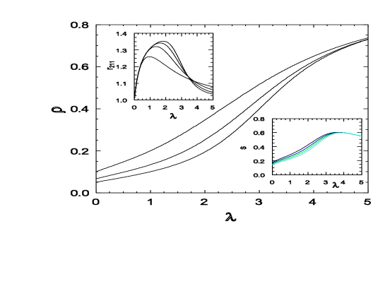
Figure 1: QS order parameter vs. creation rate $\lambda$ in the CP; system sizes $L=10$, 15 and 20 (upper to lower). Upper inset: moment ratio $r_{211}$ for system sizes 5, 10, 15, and 20, in order of increasing maximum value. Lower inset: entropy per site $s$ for sizes 17, 19, 21, and 23 (left to right).

I determined the QSD for the contact process on rings of up to 23 sites. The number of configurations scales as $N_{c}\simeq(2^{L}-2)/L+1$ (for $L$ prime this formula is exact). The number of annihilation transitions is $N_{a}\simeq 2^{L-1}$ (on average half the sites are occupied) and that of creation transitions is $N_{cr}\simeq 3\cdot 2^{L-3}$. (For $L=23$, there are 364 723 configurations, and $\approx 7.3\times 10^{6}$ transitions; the calculation takes about 16 hours on a 3 GHz processor.)

The QS order parameter $\rho$ (Fig. 1), follows the anticipated trend (i.e., $\rho(\lambda)$ is a sigmoidal function), but does not show any clear sign of the critical point; indeed, no such sign is expected for the small systems considered here. A precise estimate of the critical value $\lambda_{c}$ can nevertheless be obtained through analysis of the moment ratios. Let $m_{j}$ denote the $j$-th moment of the occupied site density, and $r_{211}\equiv m_{2}/m_{1}^{2}$. The values $\lambda_{r,L}$, marking the crossing of $r_{211}(L)$ and $r_{211}(L+1)$, approach the critical value systematically, as shown in Fig. 2. ($\lambda_{r,L}$ is plotted, for convenience, versus $L^{-1.5}$ as this leads to an approximately linear plot.) Once preliminary estimates of $\lambda_{r,L}$ (with uncertainty $\sim 10^{-5}$) have been obtained, I perform high-resolution studies, with $\Delta\lambda=10^{-4}$, in the vicinity of each crossing; precise estimates of the crossing values (uncertainty $\sim 10^{-13}$) are then obtained applying Neville’s algorithm numrec to the data for $r_{211}(L+1)-r_{211}(L)$. Using the Bulirsch-Stoer (BST) extrapolation technique numrec ; monroe , the data for sizes 8 to 23 furnish $\lambda_{c}=3.2961(15)$ and the critical moment ratio $r_{211,c}=1.1729(1)$. These values compare well with the best available estimates of $\lambda_{c}=3.297848(20)$ and $r_{211,c}=1.1736(1)$ qssim ; the associated errors are $\approx$ 0.05%, remarkably small, in light of the system sizes used.

Figure 2: Contact process: values of $\lambda$ at crossings of $r_{211}$ (upper set), and at kurtosis minima (lower set) versus $1/L^{1.5}$. Inset: kurtosis $q$ versus $\lambda$ for (lower to upper) $L=17$, 19, 21, and 23.

The moment ratios $r_{3111}\equiv m_{3}/m_{1}^{3}$ also exhibit crossings that converge to $\lambda_{c}$. More surprisingly, the product $m_{-1}m_{1}$ exhibits crossings and appears to approach a well defined limit, 1.366(1), as $L\to\infty$ at the critical point; simulations ($L=1000$ and 2000), yield 1.374(2) for this quantity. The reduced fourth cumulant, or kurtosis, given by $q(\lambda,L)=K_{4}/K_{2}^{2}$, where $K_{2}=m_{2}-m_{1}^{2}$ (the variance of the order parameter) and $K_{4}=m_{4}-4m_{3}m_{1}-3m_{2}^{2}+12m_{2}m_{1}^{2}-6m_{1}^{4}$, does not exhibit crossings but instead takes a pronounced minimum at a value $\lambda_{qm}(L)$ that converges to the critical value as $\lambda_{c}-\lambda_{qm}(L)\propto L^{-1.39(1)}$. (This property has been verified in simulations using $L=1000$, and 2000; departures from the minimum value are evident for $|\Delta|=5\times 10{-4}$ inprog .) The sharpness of the minimum, as gauged by $q^{\prime\prime}=d^{2}q/d\lambda^{2}|_{\lambda_{qm}}$, appears to increase rapidly with size: $q^{\prime\prime}\propto L^{1.84(3)}$. (This is consistent with $q^{\prime\prime}\sim L^{2/\nu_{\perp}}$, as expected from FSS.) Since a negative kurtosis reflects a probability distribution that is broader at the maximum, and with shorter tails (compared to a Gaussian distribution with the same mean and variance), it is natural that $q$ should be minimum at the critical point, where fluctuations are dominant.

The statistical entropy per site, $s=-L^{-1}\sum_{j}p_{j}\ln p_{j}$, is plotted in Fig. 1. In the large-$L$ limit, $s$ should be zero for $\lambda<\lambda_{c}$, since the QSD is concentrated on a set of configurations with vanishing density. As $L\to\infty$, one expects $ds/d\lambda|_{\lambda_{c}}$ to diverge (as is the case for $d\rho/d\lambda$), and to attain a maximum at some $\lambda>\lambda_{c}$, approaching zero as $\lambda\to\infty$. The numerical data are consistent with these trends.

Figure 3: Main graph: finite differences $\Delta\ln\rho/\Delta\ln L$ versus $1/L$ in the CP (upper set) and PCP (lower set); left inset: finite differences $\Delta\ln r_{1}/\Delta\ln L$ (symbols as in main graph); right inset: order parameter in CP at $\lambda_{c}$ versus system size, on log scales.

Encouraged by the good results of the moment-ratio analysis, I examine three quantities expected, on the basis of FSS, to exhibit scaling at the critical point: the QS lifetime $\tau$, the order parameter, and the derivative $r^{\prime}\equiv|dr_{211}/d\lambda|$. (The latter should diverge $\propto L^{1/\nu_{\perp}}$.) Despite the small system sizes, these quantities indeed appear to follow power laws (see Fig. 3). To obtain precise estimates of the associated exponents, I calculate the finite difference ratios $\Delta\ln\rho/\Delta\ln L=[\ln\rho(L)-\rho(L-1)]/[\ln L-\ln(L-1)]$, (and similarly for $\tau$ and $r^{\prime}$). Linear regression of these ratios versus $1/L$, using the seven largest sizes, yields $\beta/\nu_{\perp}=0.25193(3)$, $z=1.58054(2)$, and $\nu_{\perp}=1.092(1)$. These estimates differ by 0.06%, 0.01%, and 0.5%, respectively, from the literature values of 0.25208, 1.5807, and 1.0968 jensen99 . Thus data on QS properties of systems with 23 sites or fewer yield estimates of critical exponents to within half a percent or better! Precise estimates are also found for $r_{3111}$ and $q$ at the critical point: using BST extrapolation I find values of 1.5306(5) and -0.5015(5), compared with the simulation values of 1.526(3) and -0.505(3), respectively rdjaff .

To test the robustness of this approach, I apply it to the pair contact process (PCP). In the PCP jensen93 , each site is again either occupied or vacant, but all transitions involve a pair of particles occupying nearest-neighbor sites, called a pair in what follows. A pair annihilates itself at rate $p$, and with rate $1-p$ creates a new particle at a randomly chosen site neighboring the pair, if this site is vacant. Any configuration lacking a pair of nearest-neighbor occupied sites is absorbing. Simulation results jensen93 ; iwanrdpcp ; rdjaff place the PCP in the same universality class as the CP (namely, that of directed percolation). Unlike the CP, for which quite precise results have been derived via series expansions, there are no reliable predictions from series or other analytic methods.

Using, as before, the parameter values associated with crossings of the moment ratio $m_{211}$, I obtain (for system sizes $L=8$ to 23), the estimate $p_{c}=0.07330(3)$, about 0.3% above the best available estimate of 0.077092(1) pcpdqss . The estimates $\beta/\nu_{\perp}=0.2483(1)$ and $\nu_{\perp}=1.096(2)$, obtained via the same procedure as used for the CP, are also in good agreement with the accepted values. Analysis of the QS lifetime however, yields the unexpectedly large value $z\simeq 2.6$. In fact, the finite-difference ratios $\Delta\ln\tau/\Delta\ln L$ vary erratically with $L$, indicating that the result for $z$ is unreliable. This may be associated with the large number of absorbing configurations in the PCP (growing exponentially with $L$), so that the extinction rate has not reached its asymptotic limiting behavior at the system sizes considered here. Extrapolation of the moment ratio at $p_{c}$ yields $m_{122}=1.174(1)$, and reduced fourth cumulant $q=-0.500(5)$, again in good accord with the expected values. (As in the case of the CP, the value of $\lambda$ at which $q$ takes its minimum approaches $\lambda_{c}$ with increasing system size.) Thus the QS properties of the PCP (for $L\leq 23$) permit one to assign the model to the directed percolation class, despite the lack of a clear result for the dynamic exponent $z$.

It is natural to inquire whether the QS probability distribution exhibits any simplifying features. In an equilibrium lattice gas with interactions that do not extend beyond nearest neighbors, for example, the probability of a configuration depends only on the number of particles $N$ and nearest-neighbor pairs $P$. The the CP, by contrast, I find that the QS probability of each configuration in a given $(N,P)$ class is distinct (the probabilities typically vary over an order of magnitude or more, even far from the critical point). In a broad sense, this is because, unlike in equilibrium, not all annihilation events possess a complementary creation event. For similar reasons, it does not appear likely that the QSD could be obtained via the maximization of the statistical entropy, subject to some simple set of constraints.

In summary, I show that analysis of exact (numerical) quasistationary properties on relatively small rings yields remarkably precise results for critical properties at an absorbing-state phase transition. Deriving the QS distribution involves rather modest programming and computational effort: the results reported here can be obtained in a few days on a fast microcomputer. Applied to the contact process, the analysis yields most critical properties with an error well below 0.1%. For the more complicated PCP, errors are generally $\leq$ 1%. Application to other absorbing-state phase transitions, including some belonging to other universality classes, is in progress. The method may also be useful in the study of metastable states, provides a valuable check on simulations, and may serve as the basis for phenomenological renormalization group approaches.

Acknowledgment

I thank Robert Ziff for valuable suggestions. This work was supported by CNPq and FAPEMIG, Brazil.

References

- (1) N. G. van Kampen, Stochastic Processes in Physics and Chemistry (North-Holland, Amsterdam, 1992).
- (2) C. W. Gardiner, Handbook of Stochastic Methods, (Springer-Verlag, Berlin, 1990).
- (3) T. E. Harris, Ann. Probab. 2, 969 (1974).
- (4) T. Liggett, Interacting Particle Systems (Springer-Verlag, Berlin, 1985).
- (5) R. Dickman, M. A. Muñoz, A. Vespignani, and S. Zapperi, Braz. J. Phys. 30, 27 (2000).
- (6) T. Bohr, M. van Hecke, R. Mikkelsen, and M. Ipsen, Phys. Rev. Lett. 86, 5482 (2001), and references therein.
- (7) J. Marro and R. Dickman, Nonequilibrium Phase Transitions in Lattice Models (Cambridge University Press, Cambridge, 1999).
- (8) H. Hinrichsen, Adv. Phys. 49 815, (2000).
- (9) G. Ódor, Rev. Mod. Phys 76, 663 (2004).
- (10) S. Lübeck, Int. J. Mod. Phys. B 18, 3977 (2004).
- (11) K. A. Takeuchi, M. Kuroda, H. Chaté, and M. Sano, eprint: arXiv:0706.4151.
- (12) R. Dickman and R. Vidigal, J. Phys. A 35, 1145 (2002).
- (13) M. M. de Oliveira and R. Dickman, Phys. Rev. E 71, 016129 (2005).
- (14) R. Dickman and M. M. de Oliveira, Physica A 357, 134 (2005); M. M. de Oliveira and R. Dickman, Braz. J. Phys. 36, 685.
- (15) F. Ginelli, H. Hinrichsen, R. Livi, D. Mukamel, and A. Torcini J. Stat. Mech. 2006, P08008.
- (16) R. Dickman, Phys. Rev. E 65, 047701 (2002).
- (17) I. Jensen and R. Dickman, J. Stat. Phys. 71, 89 (1993).
- (18) M. E. Fisher and M. N. Barber, Phys. Rev. Lett. 28, 1516 (1972).
- (19) W. Press, S. Teukolsky, W. Vetterling, and B. Flannery, Numerical Recipes (Cambridge University Press, Cambridge, 1992.).
- (20) J. L. Monroe, Phys. Rev. E65, 066116 (2002).
- (21) Detailed results on moment ratios will be reported elsewhere.
- (22) I. Jensen, J. Phys. A 32, 5233 (1999).
- (23) R Dickman and J. Kamphorst Leal da Silva, Phys. Rev. E58, 4266 (1998).
- (24) I. Jensen, Phys. Rev. Lett. 70, 1465 (1993).
- (25) I. Jensen and R. Dickman, Phys. Rev. E48, 1710 (1993).
- (26) M. M. de Oliveira and R. Dickman, Phys. Rev. E 74, 011124 (2006).