Order parameter for the dynamical phase transition in Bose-Einstein condensates with topological modes

Abstract

In a trapped Bose-Einstein condensate, subject to the action of an alternating external field, coherent topological modes can be resonantly excited. Depending on the amplitude of the external field and detuning parameter, there are two principally different regimes of motion, with mode locking and without it. The change of the dynamic regime corresponds to a dynamic phase transition. This transition can be characterized by an effective order parameter defined as the difference between fractional mode populations averaged over the temporal period of oscillations. The behavior of this order parameter, as a function of detuning, pumping amplitude, and atomic interactions is carefully analyzed. A special attention is payed to numerical calculations for the realistic case of a quadrupole exciting field and the system parameters accessible in current experiments.

I Introduction

Bose-Einstein condensation (BEC) in weakly interacting dilute Bose gases is a topic of high current interest and intensive investigations, both experimental and theoretical, as can be inferred form the book Pitaevskii03 and review articles Dalfovo99 ; Courteille01 ; Yukalov04 ; Andersen04 ; Bongs04 ; Yukalov05 ; Posazhennikova06 . At sufficiently low temperature, the weakly interactiong gas is almost completely Bose-condensed and is well described by the Gross-Pitaevskii equation Pitaevskii03 . Then the system is in its ground state. One could pose a question whether nonground-state Bose-Einstein condensates could be realized?

The possibility of creating nonground-state Bose-Einstein condensates was advanced in Ref. Yukalov97 . As is clear, such a condensate has to be nonequilibrium, since in an equilibrium system at zero temeprature, the state with the lowest energy would be always preferable. The most important point is that the atomic system would possess a discrete spectrum, or at least, would have finite gaps between different parts of its spectrum, such as occur in optical lattices. A straightforward way of obtaining a purely discrete spectrum is by confining atoms in a trapping potential. Then, in order to transfer atoms from their ground BEC state to another nonground level, the system has to be subject to an oscillatory external field. The field oscillation is to be close to the frequency of the transition between the ground and the chosen excited state of the trap. The states of the trapped coherent atomic cloud are given by the set of solutions to the stationary Gross-Pitaevskii equation, which are termed topological coherent modes. Due to the nonlinearity of the system, caused by atomic interactions, the spectrum is not equidistant and allows for the selection of the desired levels by means of the resonant modulation of an external field. It has been mathematically accurately proved Yukalov97 ; Yukalov02 that this resonantly excited condensate can be well approximated by an effective two-level system. The analytical proof has been confirmed Yukalov-Marzlin04 by direct numerical simulations for the time-dependent Gross-Pitaevskii equation. The topological coherent modes have also been studied theoretically in Refs. Ostrovskaya00 ; Kivshar01 ; D'Agosta02 ; D'Agosta-Presilla02 ; Proukakis02 ; Adhikari04 . The generation of a nonground-state BEC has recently been observed in optical lattices Muller07 .

The resonant system with nonground-state BEC, generated by an applied modulating field, possesses several unusual properties, as is reviewed in Ref. Yukalov06 . One of the interesting features is the existence of two essentially different regimes of motion. In one of them, the fractional mode populations are locked in the regions close to their initial conditions, while in another regime, the mode populations oscillate in the whole diapason between zero and one. The transition between these two dynamical regimes represents a kind of a dynamic phase transition. It has been shown Yukalov00 ; Yukalov01 ; Yukalov-Yukalova02 that this dynamical transition is equivalent to a phase transition in an effective averaged system, accompanied by critical phenomena around the phase transition. According to Landau and Lifshitz Landau80 , an order parameter is a quantity defined in such a way that it takes non-zero values, positive or negative, in the unsymmetrical phase and is zero in the symmetrical phase. So, similarly to phase transitions in equilibrium systems, it is possible to define an order parameter characterizing the dynamic phase transition. The role of such an order parameter for the system with resonantly generated topological modes is played by the difference between the time-averaged mode populations for the ground and the excited states.

The aim of the present work is twofold. First, we analyze the order-parameter behavior for a wide range of different values of the detuning, pumping, and interaction strengths. Second, we accomplish a numerical investigation of the order-parameter features for a setup typical for current experiments, so that to choose realistic conditions for experimentally realizing the discussed generation of the coherent topological modes and observing the dynamic phase transition between the mode-locked and unlocked regimes.

The structure of the paper is as follows. In Section II, we recall the main equations describing the resonant excitation of the coherent topological modes Yukalov97 ; Yukalov01 , characterizing the coupling between the ground and excited states of BEC. In Section III, we present the results of our investigation for the behavior of the order parameter under the varying amplitude of the excitation field, detuning from resonance, and for different strengths of atomic interactions. In section IV, we explore the case of a realistic alternating field that could be realized in experiment, for which we consider an oscillatory magnetic quadrupole field. We summarize our results in the concluding section .

II Main Equations and Definition of Model

The mathematical model, rather accurately describing a trapped BEC of a dilute Bose gas, is the well-known Gross-Pitaevskii equation Dalfovo99 , which is equivalent to the nonlinear Schrödinger equation

$$\hat{H}[\Phi]\Phi=i\hslash\frac{\partial\Phi}{\partial t},\qquad\hat{H}[\Phi]=-\frac{\hslash^{2}}{2m_{0}}\nabla^{2}+U_{trap}\left(\mathbf{r}\right)+A_{s}\left|\Phi\right|^{2},$$ (1)

where $U_{trap}\left(\mathbf{r}\right)$ is the trapping potential, $A_{s}=4\pi(N-1)\hslash^{2}a_{s}/m_{0}$, with $m_{0}$ being atomic mass; $a_{s}$, the s-wave scattering length; and $N$, the number of atoms. The stationary wave-function $\Phi$ can be written in the form

$$\Phi_{n}=\Phi_{n}\left(\mathbf{r},t\right)=\varphi\left(\mathbf{r}\right)e^{-iE_{n}t/\hslash},$$ (2)

where $\varphi_{n}\left(\mathbf{r}\right)$ is a solution to the stationary Gross-Pitaevskii equation

$$\hat{H}[\varphi_{n}]\varphi_{n}=E_{n}\varphi_{n}.$$ (3)

Since the Hamiltonian in equation (3) is non-linear, the spectrum $E_{n}$ is not equally spaced Yukalov97 . Because of this, it is possible to couple the ground BEC state in the confining potential to another mode (labeled $p$) by applying an oscillatory field Yukalov97 , e.g., given by

$$V_{p}\left(\mathbf{r},t\right)=V\left(\mathbf{r}\right)cos(\omega t),$$ (4)

where $\omega$ is the angular frequency characterizing the time variation of the field and $V\left(\mathbf{r}\right)$ is a spatially dependent amplitude. If this frequency is chosen to be close to the transition frequency between the two modes, then, as has been shown Yukalov97 ; Yukalov02 , the total wave-function $\Phi$ can be written as the sum of two modes

$$\Phi\left(\mathbf{r},t\right)=c_{0}\left(t\right)\varphi_{0}\left(\mathbf{r}\right)e^{-iE_{0}t/\hslash}+c_{p}\left(t\right)\varphi_{p}\left(\mathbf{r}\right)e^{-iE_{p}t/\hslash},$$ (5)

where the population $n_{j}$ of each mode is given by

$$n_{j}=|c_{j}(t)|^{2}.$$ (6)

This implies that if we wish to know the temporal evolution of these mode populations, we need to find out how the coefficients $c_{j}$ evolve in time. Substituting Eq. (5) into the Schrödinger equation

$$\left[\hat{H}+V\left(\mathbf{r},t\right)\right]\Phi\left(\mathbf{r},t\right)=i\hslash\frac{\partial\Phi\left(\mathbf{r},t\right)}{\partial t},$$ (7)

we obtain the rate equations for the coefficients $c_{0}$ and $c_{p}$,

$$\frac{dc_{0}}{dt} = -i\alpha_{0p}n_{p}c_{0}-\frac{i}{2}\beta e^{i\Delta\omega t}c_{p},$$ (8a)

$$\frac{dc_{p}}{dt} = -i\alpha_{p0}n_{0}c_{p}-\frac{i}{2}\beta^{*}e^{-i\Delta\omega t}c_{0}.$$ (8b)

An accurate derivation of these rate equations can be done Yukalov97 ; Courteille01 ; Yukalov02 by employing the Krylov-Bogolubov averaging technique Bogolubov61 . In Eq. (8), we have the transition amplitude, defined as

$$\alpha_{jk}=\frac{A_{s}}{\hslash}\int|\varphi_{j}\left(\mathbf{r}\right)|^{2}\left(2|\varphi_{k}\left(\mathbf{r}\right)|^{2}-|\varphi_{j}\left(\mathbf{r}\right)|^{2}\right)d\mathbf{r},$$ (9)

the coupling amplitude caused by the external field, defined as

$$\beta=\frac{1}{\hslash}\int\varphi_{0}^{*}\left(\mathbf{r}\right)V\left(\mathbf{r}\right)\varphi_{p}\left(\mathbf{r}\right)d\mathbf{r},$$ (10)

and the detuning $\Delta\omega=\omega-\omega_{p,0}$, which is the difference between the field frequency and the transition frequency, given by $\hslash\,\omega_{p,0}=E_{p}-E_{0}$. Note that amplitude (9) is unsymmetric, i.e., not necessarily $\alpha_{0p}=\alpha_{p0}$. It comes from the non-linearity introduced by interaction. The interaction will have different values depending on the occupied state and that may be the cause of the obtained unsymmetry in $\alpha_{jk}$.

Our physical system is similar to a condensate in a double-well potential. Here, the coupling field characterized by the parameter $\beta$ has the role of tunneling and there is the same nonlinear term associated with collisions. Instead of using the two-mode model Milburn97 , we prefer to use the Gross-Pitaevskii formalism which predict the form of the spatial distributions of wave function for both, ground and excited, condensates.

The system of equations (8) can be solved numerically for each given set of parameters. In order to simplify the description, the following dimensionless parameters are introduced:

$$a=\frac{\alpha_{0p}}{\alpha_{p0}},\qquad b=\frac{\beta}{\alpha_{p0}},\qquad\delta=\frac{\Delta\omega}{\alpha_{p0}},$$ (11)

with the time scaling

$$t^{\prime}=\alpha_{p0}\,t.$$ (12)

This system of equations allows us to find the temporal behavior of the mode amplitudes characterizing the fractional mode populations (6) Yukalov97 ; Yukalov00 . In Fig. 1, we present the temporal evolution of the mode populations for a resonant field ($\delta=0$), the interaction amplitude $a=1$, and different values of the pumping amplitude $b$. We assume that, initially, all atoms are in the ground-state BEC, i. e., $c_{0}(0)=1$ and $c_{p}(0)=0$.

Figure 1: Time evolution of the population fraction of the ground state (solid line) and the excited state (dashed line) in the presence of a resonant field, $\delta=0$, and $a=1$ for (a) $b=0.4$; (b) $b=0.5$; (c) $b=0.5001$; (d) $b=0.6$.

We see that there are two different types of behavior of the population dynamics. For $b<0.5$, the ground state population is always larger than that of the excited state. While for $b>0.5$, the time averages of both population modes are the same, which means that it is possible to transfer all atoms from the ground to the excited state. The same effect can be obtained for other values of $a$ as we can see in Fig. 2, with $a=0.1$ and a detuning $\delta=0.45$.

Figure 2: Time evolution of the population fraction in the ground state (solid line) and the excited state (dashed line) in the presence of a field with the detuning $\delta=0.45$ and $a=0.1$ for (a) $b=0.2$; (b) $b=0.2749$; (c) $b=0.2750$; (d) $b=0.4$.

As is seen, it is easier to detect a trapped BEC in an excited state, when the dynamics correspond to the mode-unlocked regime shown in the cases (c) and (d) of Figs. 1 and 2, since in these cases the system stays longer in the excited state. In order to deeper understand how the excitation depends on the parameters of the system, it is useful to analyze the behavior of the order parameter, as defined in Refs. Yukalov01 ; Yukalov-Yukalova02 .

III Order Parameter for Dynamic Transition

The order parameter, characterizing the dynamic phase transition for the case of the resonant BEC, with the generated topological modes, can be defined Yukalov01 , as the difference $\eta$ between the time-averaged fractional mode populations,

$$\eta=\overline{n}_{0}-\overline{n}_{p},$$ (13)

where $\overline{n}_{i}$ is the time average of $n_{i}$ over the whole oscillation period. This order parameter clearly shows us what kind of dynamic regime occurs. Observing the character of the mode oscillations, we note that in cases (a) and (b) of Fig. 1 and Fig. 2, $\eta>0$, and in the (c) and (d) cases, $\eta=0$.

We have calculated the behavior of $\eta$ as a function of $b$, for $0\leq a\leq 2$ with different amplitudes of the resonant field. These results are shown in Fig. 3, from where we see that there is an abrupt change of the order parameter for $a\geq 0.8$, while for $a\leq 0.8$, $\eta$ goes smoothly to zero. Also, for $0.8\leq a<1$, $\eta$ becomes negative for some values of $b$. When the order parameter is negative, this does not mean that the fraction of the excited mode is always larger than the ground state population. It simply shows that the BEC on the average spends more time in the excited state, which would favor the detection of condensed atoms in that state.

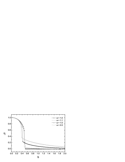
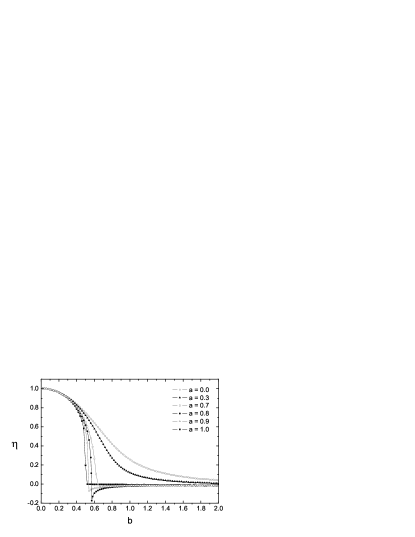
Figure 3: Order parameter $\eta$ as a functions of $b$ for different values of $a$ with a resonant field excitation.

To better illustrate the peculiarities of the population evolution, we show in Fig. 4 the mode populations $n_{0}$ and $n_{p}$, for $a=0.8$, for different values of $b$. In all these cases we set the resonant external field ($\delta=0$). As presented in Fig. 3 and Fig. 4, when $a=0.8$ and $b=0.57$, we have $\eta\simeq-0.174$. Then $n_{p}$ never reaches one, i. e., we do not get a completely excited BEC. For conditions presented in Fig. 4(d), the excited state population is dominant for the major part of time.

Figure 4: Fractions of mode populations in the ground state (solid line) and the excited state (dashed line) in the presence of a resonant field, $\delta=0$, and $a=0.8$ for (a) $b=0.55$; (b) $b=0.56$; (c) $b=0.565$; (d) $b=0.57$.

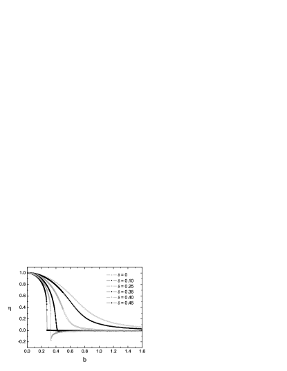
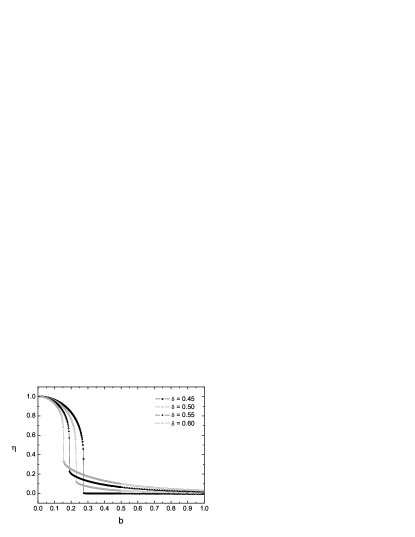
Figure 5: Order parameter $\eta$ as a function of $b$ for different values of $\delta$ with $a=0.1$.

The behavior of the order parameter when varying the detuning for a fixed interaction strength $a=0.1$ is presented in Fig. 5, which shows $\eta$ as a function of $b$ for different values of the detuning. This figure, together with Fig. 3, characterizes the overall behavior of the order parameter under varying the system parameters $a$, $b$ and $\delta$.

The question that is yet left open is how and under what particular conditions the proposal of obtaining the dynamical phase transition for a trapped BEC Yukalov01 could be realized in laboratory. To this end, we need to study the behavior of the order parameter $\eta$ for a realistic setup of the applied field geometry, field amplitude, and detuning, so that to identify the critical field that changes the dynamic regime of the mode excitation. The specifications for the dimensionless parameters $a$, $b$, and $\delta$ for a typical laboratory setup is, therefore, necessary. In the following section, we calculate these parameters for a magnetic quadrupole field, which corresponds to the experiment in progress in our group, employing a ${}^{87}Rb$ condensate.

IV Magnetic Quadrupole as an Excitation Field

The amplitudes $\alpha_{0p}$, $\alpha_{p0}$, and $\beta$ cannot be obtained as exact analytic expressions, since there are no exact analytic solutions for the Gross-Pitaevskii equation. We can, however, obtain rather accurate approximate solutions using the Optimized Perturbation Theory Yukalov76 , whose detailed description can be found, e.g., in Ref. Courteille01 . In this case, approximate expressions for the ground state and three excited-state wave functions, for a harmonic trap

$$U_{trap}=\frac{1}{2}\left(\omega_{r}^{2}\,r^{2}+\omega_{z}^{2}z^{2}\right),$$ (14)

are given by

$$\phi_{000} = \left(\frac{u_{000}^{2}v_{000}}{\pi^{3}l_{r}^{6}}\right)^{1/4}e^{-(u_{000}r^{2}+v_{000}z^{2})/2l_{r}^{2}},$$ (15)

$$\displaystyle\phi_{010} = u_{010}\left(\frac{v_{010}}{\pi^{3}l_{r}^{6}}\right)^{1/4}\frac{r}{l_{r}}e^{i\varphi}e^{-(u_{010}r^{2}+v_{010}z^{2})/2l_{r}^{2}},$$ (16)

$$\displaystyle\phi_{001} = \left(\frac{4u_{001}^{2}v_{001}^{2}}{\pi^{3}l_{r}^{6}}\right)^{1/4}\frac{z}{l_{r}}e^{-(u_{001}r^{2}+v_{001}z^{2})/2l_{r}^{2}},$$ (17)

$$\phi_{100} = \left(\frac{u_{100}^{2}v_{100}}{\pi^{3}l_{r}^{6}}\right)^{1/4}\left(1-u_{100}\frac{r^{2}}{l_{r}^{2}}\right)e^{-(u_{100}r^{2}+v_{100}z^{2})/2l_{r}^{2}},$$

where $l_{r}=\sqrt{\hslash/m_{0}\omega_{r}}$ is the oscillator length, and $u_{nmk}$ and $v_{nmk}$ are the variational parameters, defined by minimizing the corresponding energy of each mode.

The alternating magnetic field in a magnetic trap can be created as an oscillatory quadrupole magnetic field of the form

$$\textbf{B}(\textbf{r},t)=\left(Ax\hat{x}+Ay\hat{y}-2Az\hat{z}\right)cos\omega t,$$ (19)

which corresponds to the field formed by a pair of coils operating in the anti-Helmholtz configuration. Then the potential $V(\textbf{r})$ in Eq. (4) is given by

$$V(\textbf{r})=-\vec{\mu}\cdot\textbf{B}=g_{F}\,m_{F}\,\mu_{B}\,A\,\sqrt{r^{2}+4z^{2}},$$ (20)

where $\vec{\mu}$ is the atomic magnetic moment, $g_{F}$ is the gyromagnetic factor, $m_{F}$ is the magnetic quantum number, and $\mu_{B}$ is the Bohr’s magneton. It is easy to see that the sole topological mode, from the lowest modes given above, which could be coupled to the ground-state mode by the potential (20), is the radial dipole mode $\phi_{100}$. For this mode, we have made calculations of the order parameter $\eta$ as a function of the field-amplitude parameter $A$. We have chosen this parameter $A$ because it is easily controllable in laboratory, since it is proportional to the current in the coils constructed to produce the desired field Bergeman87 .

We set all parameters of the system according to the experiment in progress, where ${}^{87}Rb$ is employed, having mass $m_{0}=0.144\times 10^{-21}\,g$ and the scattering length $a_{s}\simeq 6nm$. The magnetic trap has $\omega_{r}=2\pi\times 120\,Hz$ and $\omega_{z}=2\pi\times 24\,Hz$. The number of atoms is taken as $N=10^{4}$, which corresponds to a realistic experimental number. Figure 6 shows the obtained results for different detunings. In this case, the transition frequency between the ground state and the radial dipole mode is $\omega_{100,0}=2\pi\times 190\,Hz$.

Figure 6: Order parameter $\eta$ for the exciting magnetic quadrupole field as a function of the field parameter $A$ for different values of the field detuning.

This figure clearly shows that there exist critical points in the behavior of $\eta$, which depend on the detuning. In Fig. 6, when, for instance, $\Delta\omega=-2\pi\times 2\,Hz$, the critical point happens for $A=0.096\,G/cm$. Three different situations are seen in Fig. 6. For $\Delta\omega=-2\pi\times 13\,Hz$, we have the situation similar to that for $a=0.1$ and $\delta=0.40$, shown in Fig. 5, when $\eta<0$. In this case, the critical point occurs when $A\simeq 0.119\,G/cm$. We also have the case when the critical point occurs for $\eta>0$, which is analogous to the behavior obtained for $a=0.1$ and $\delta>0.45$ and shown in Fig. 5. Here, for $\Delta\omega=2\pi\times 13\,Hz$, the critical point happens for $A\simeq 0.068\,G/cm$. In the case of a negative detuning, $\Delta\omega=-2\pi\times 36\,Hz$, there is no abrupt change in the behavior of $\eta$, similarly to the case shown in Fig. 5, where a resonant field is considered.

V Conclusion

The dynamics of the resonant excitation of topological coherent modes of a Bose-Einstein condensate in a harmonic trap is analyzed. The behavior of the effective order parameter is investigated as a function of the external field amplitude for a variety of different system characteristics, such as the detuning from the resonance and interaction amplitudes. An important observation is that the detuning can compensate the influence of atomic interactions, producing in the case of a weak interaction ($a=0.1$), the behavior similar to that obtained for a strong interaction ($a=1$) and a purely resonant field. The pumping field, in the setup of the quadrupolar geometry was employed to study the feasibility of observing the dynamic phase transition for typical experimental conditions. The frequency variation around the resonance leads to the different behavior of the order parameter, depending on whether the detuning is red- or blue- shifted. The obtained results can be used for the experimental realization of the dynamic phase transition in the process of resonant generation of topological coherent modes.

Finally, we shall mention that several calculation using Bogoliubov theory performed by Dziarmaga and Sacha Dziarmaga03 shown that the effect of quantum and thermal depletion could be a serious limitation on quantum coherence of atomic BEC. Second question is the necessity of an efficient atomic population transference. If both, quantum and thermal depletion, affect the process, we cannot guarantee that the atoms which populates the excited state are a Bose-Einstein condensate (a coherent state). Following Ruostekoski and Walls Ruostekoski98 , the effects of decoherence due to noncondensed atoms on BECs shows that purity decays fast. Hence, one must have the interaction parameter much smaller than the decoherence time scale associated with the nonlinear parameter. Because our analysis shown that the macroscopic population of the excited state is associated with small values of b, we believe the effects of decoherence will be small.

- (1) L. Pitaevskii and S. Stringari, Bose-Einstein Condensation (Clarendon, Oxford, 2003).
- (2) F. Dalfovo, S. Giorgini, L. P. Pitaevskii, and S. Stringari Rev. Mod. Phys. 71, 463 (1999).
- (3) P. W. Courteille, V. S. Bagnato, and V. I. Yukalov, Laser Phys. 11, 659 (2001).
- (4) V. I. Yukalov, Laser Phys. Lett. 1, 435 (2004).
- (5) J. O. Andersen, Rev. Mod. Phys. 76, 599 (2004).
- (6) K. Bongs and K. Sengstock, Rep. Prog. Phys. 67, 907 (2004).
- (7) V. I. Yukalov and M. D. Girardeau, Laser Phys. Lett. 2, 375 (2005).
- (8) A. Posazhennikova, Rev. Mod. Phys. 78, 1111 (2006).
- (9) V. I. Yukalov, E. P. Yukalova, and V. S. Bagnato, Phys. Rev. A 56, 4845 (1997).
- (10) V. I. Yukalov, E. P. Yukalova, and V. S. Bagnato, Phys. Rev. A 66, 043602 (2002).
- (11) V. I. Yukalov, K. P. Marzlin, and E. P. Yukalova, Phys. Rev. A 69, 023620 (2004).
- (12) E. A. Ostrovskaya, Y. S. Kivshar, M. Lisak, B. Hall, F. Cattani, and D. Anderson, Phys. Rev. A 61, 031601(R) (2000).
- (13) Y. S. Kivshar, T. J. Alexander, and S. K. Turytsin, Phys. Lett. A 278, 225 (2001).
- (14) R. D’Agosta, B. A. Malomed, and C. Presilla, Laser. Phys. 12, 37 (2002).
- (15) R. D’Agosta and C. Presilla, Phys. Rev. A 65, 043609 (2002).
- (16) N. P. Proukakis and L. Lambropoulos, Eur. Phys. J. D 19, 355 (2002).
- (17) S. K. Adhikari, Phys. Rev. A 69, 063613 (2004).
- (18) T. Müller, S. Fölling, A. Widera, and I. Bloch, e-print arXiv:0704.2856.
- (19) V. I. Yukalov, Laser Phys. Lett. 3, 406 (2006).
- (20) V. I. Yukalov, E. P. Yukalova, and V. S. Bagnato, Laser Phys. 10, 26 (2000).
- (21) V. I. Yukalov, E. P. Yukalova, and V. S. Bagnato, Proc. SPIE 4243, 150 (2001).
- (22) V. I. Yukalov, E. P. Yukalova, and V. S. Bagnato, Laser Phys. 12, 231 (2002).
- (23) L. D. Landau and E. M. Lifshitz, Statistical Physics (Pergamon Press, Oxford, 1980).
- (24) N. N. Bogolubov and Y. A. Mitropolsky, Asymptotic Methods in the Theory of Nonlinear Oscillations (Gordon and Breach, New York, 1961).
- (25) G. J. Milburn, J. Corney, E. M. Wright, and D. F. Walls, Phys. Rev. A 55, 4318 (1997).
- (26) V. I. Yukalov, Moscow Univ. Phys. Bull. 31, 10 (1976).
- (27) For more details about the derivation of the field-parameter , see T. Bergeman, G. Erez, and H. J. Metcalf, Phys. Rev. A 35, 1535 (1987).
- (28) J. Dziarmaga and K. Sacha, Phys. Rev. A 68, 043607 (2003).
- (29) J. Ruostekoski and D. F. Walls, Phys. Rev. A 58, R50 (1998).