Using GRO J1655-40 to test Swift/BAT as a monitor for bright hard X-ray sources

Abstract

Context. While waiting for new gamma-ray burst detections, the Burst Alert Telescope (BAT) onboard Swift covers each day $\sim$50% of the sky in the hard X-ray band (“Survey data”). The large field of view (FOV), high sensitivity and good angular resolution make BAT a potentially powerful all-sky hard X-ray monitor, provided that mask–related systematics can be properly accounted for.

Aims. We have developed and tested a complete procedure entirely based on public Swift/BAT software tools to analyse BAT Survey data, aimed at assessing the flux and spectral variability of bright sources in the 15-150 keV energy range.

Methods. Detailed tests of the capabilities of our procedure were performed focusing, in particular, on the reliability of spectral measurements over the entire BAT FOV. First, we analyzed a large set of Crab observations, spread over $\sim$7 months. Next, we studied the case of GRO J1655-40, a strongly variable source, which experienced a 9-month long outburst, beginning on February 2005. Such an outburst was systematically monitored with the well-calibrated PCA and HEXTE instruments onboard the RXTE mission. Thanks to the good BAT temporal coverage of the source, we have been able to cross-check BAT light-curves with simultaneous HEXTE ones.

Results. The Crab tests have shown that our procedure recovers both the flux and the source spectral shape over the whole FOV of the BAT instrument. Moreover, by cross-checking GRO J1655-40 light-curves obtained by BAT and HEXTE, we found the spectral and flux evolution of the outburst to be in very good agreement. Using our procedure, BAT reproduces HEXTE fluxes within a 10-15% uncertainty with a $3\sigma$ sensitivity of $\sim 20$ mCrab for an on-axis source, thus establishing its capability to monitor the evolution of relatively bright hard X-rays sources.

1 Introduction

The Burst Alert Telescope (BAT; (Barthelmy et al. 2005)), the gamma-ray instrument on board Swift (Gehrels et al. 2004)is a highly sensitive coded mask instrument optimized in the 15-150 keV energy range. Its large ($\sim$ 2 sr) D-shaped FOV allows for the coverage of $\sim$ 1/6 of the sky in a single pointing. BAT was designed to be an efficient detector for Gamma-Ray Bursts (GRBs) and is now fulfilling its pre-launch expectations, delivering $\sim$ 100 GRBs/yr .

While waiting for new GRBs, BAT collects a huge amount of data on the hard X-ray sky. Indeed, a sensitive all-sky survey in the 15-150 keV energy range will be one of the major outcomes of the Swift mission. With an expected limiting flux of $\sim 0.2$ mCrab at high Galactic latitude and $\sim 3$ mCrab at low Galactic latitude (with a 4-year dataset), the Swift survey is expected to be $\sim$10 times deeper than the HEAO1 A4 reference all-sky hard X-ray survey (Levine et al. 1984), performed more than 25 years ago. Preliminary results, based on 3 months of data, have been published by Markwardt et al. (2005).

Owing to its large FOV, high sensitivity and good angular resolution, BAT could perform an efficient monitoring of high-energy sources. Indeed, count-rate light-curves (in the 15-50 keV energy range) for more than 400 known sources, updated on a single orbit basis, have been recently made available on the web in the “BAT Hard X-ray transient monitor” facility of the Goddard Space Flight Center (Krimm et al. 2006).

To fully exploit the data collected by BAT, however, count rate light curves should be converted into flux light curves. This would allow a continuous assessment of the varying sources’ spectral shape. Thus, we have developed a procedure aimed at extracting spectral information for bright hard X-ray sources falling into the BAT field of view.

Tests were made to verify the reliability of the results of our method, focusing on the spectral performances of the BAT instrument. First we analyzed a large number of observations of the Crab nebula (and its pulsar), the classical calibration source for X-ray instruments, performed under different observing conditions. Next, we performed a detailed study of the 9-month long 2005 outburst of the galactic microquasar GRO J1655-40. Such event was also carefully monitored with the narrow field instruments PCA and HEXTE on-board the Rossi X-Ray Timing Explorer (RXTE), making it possible to cross-check the BAT results with those obtained simultaneously by an independent well calibrated instrument.

The paper is organized as follows. After a brief overview of BAT survey data structure (section 2), we outline our automatic data analysis pipeline. The tests performed on the Crab are reported in section 3, focusing on the reliability of spectral results as a function of the source position within the BAT FOV. The requirements to combine different BAT datasets are spelled out in section 3.3.

After assessing the reliability of our pipeline using the very bright and steady Crab as a reference source, we went on to study the 2005 outburst of GRO J1655-40. Our RXTE spectral analysis is described in section 4.2. Finally, we compare BAT and RXTE spectral results, thus assessing the performances of our pipeline in order to use the BAT data to monitor the behaviour of a strongly variable source (section 4.3). Appendices A and B provide technical details on the data analysis pipelines.

2 Swift/BAT Survey Data

BAT is a coded mask instrument with a detecting area of 5200 cm². The detector is an array of 32768 CdZnTe elements operating in the 15-150 keV energy band with a good sensitivity and energy resolution (Barthelmy et al. 2005). The BAT instrument is operated in photon-counting mode. Photons interacting with the detector are processed (events) and then are tagged with an associated time of arrival, detector number and energy. Such information is stored on-board in a memory buffer which may contain $\sim$10 minutes of data (depending on the actual count rate). Data are analyzed in real time using several algorithms in order to detect new GRBs. In case of a GRB trigger, the event buffer is sent to the ground for more detailed analysis (event files), otherwise it is organized on board in a Detector Plane Histogram (DPH) and then sent to the ground. DPHs are three dimensional histograms: for a given buffer set, every cell contains the number of events received in one of 32768 pixels of the detector plane and in one of 80 energy channels. Such histograms are accumulated over a typical 5 minutes time interval and then stacked as independent rows in a “Survey” data file. Together with auxiliary files (which contain all spacecraft-related information for a given observation), they are the standard basic products for BAT non-GRB science.

All Swift data and software are publicly available and they have been downloaded at Heasarc-U.S. web site . Version 2.4 of the Swift software was used for data reduction.

3 BAT as a monitor: calibration with the Crab

BAT has a very large field of view. In order to fully exploit such a capability - which is crucial to use BAT as a monitor for the hard X-ray sky - as a first step we have to assess the stability of the source flux as reconstructed by our procedure as a function of the source position within the FOV. Indeed, different positions within the instrument FOV correspond to different mask coded fractions (see Figure  1). To this aim, we will study a large sample of observations of the bright and steady Crab, the source used to calibrate the BAT spectral response. This will be a crucial test to assess the capability of our method to extract spectral and flux information across the whole instrument FOV.

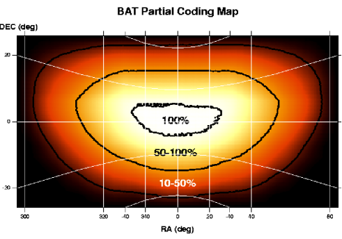
Figure 1: The D-shaped BAT Field of View. Fully coded (100%), half-coded (50%) down to the 10% coded fraction contours are indicated.

We implemented an automated data analysis pipeline based on a single-DPH row logic, i.e. extracting products for each single DPH row, following three steps.

1. “Good” data are carefully selected. Each DPH is checked for the overall count rate, pointing stability, occultations of part of the FOV by the Earth or the Moon, as well as for other possible sources of systematic effects (see Appendix A.1 for details).

2. Selected DPHs are processed to compute the source flux.

   To this aim we used the so called “Mask-weighting” technique. Such an approach is based on the “mask-weight map”, accounting for the fraction of the detector which is shadowed by the mask with respect to the source position. Applying such a mask to the DPH yields a background-subtracted spectrum of the source (for a detailed description, see Appendix A.3).

3. We also investigated the possibility to combine different DPHs, in order to increase the exposure time (and thus the source signal to noise) beyond the typical $\sim 5$ min integration of a single DPH. A careful check of the effects of DPH pointing offsets was performed, in order to assess the maximum “misjudgement” allowed to minimize flux loss in the combined DPH.

All the details of our pipeline are given in Appendix A (to study the Crab, we use steps 1,2 and 3 described there).

3.1 Data selection

Our Crab data set encompasses all observations, with the source within the BAT FOV, collected between 2005/01/01 and 2005/06/30. Such a sample includes 365 observations, including a total of 4626 DPH rows (for a total observing time of $\sim$1.46 Ms). We note that such a data set is larger than the one presented on the public BAT Digest pages describing details on the instrument calibration (44 grid locations in the BAT FOV). After the data screening stage (Appendix A.1), 1014 rows ($\sim$ 20%) were rejected. Details on the impact of each specific filtering criterium are given in Table 1.

Detectors not enabled	36
Earth contamination + SAA	121
Star tracker unlocked	264
Pointing unstable	317
High count rate	328
Earth/Moon/Sun source occultation	297

Table 1: Number of DPH rows of our Crab sample rejected after the filtering stage.

Moreover, 34 rows ($<1\%$) could not be processed owing to the lack of the relevant housekeeping files. We are then left with $\sim 3600$ good DPH rows which were used for image, as well as for spectral, analysis.

Of course, the Crab position varied greatly within the BAT FOV. Table 2 provides the statistic of the source position in the good BAT data set.

Deg off-axis	Processed rows
0-5	306
5-10	0
10-15	0
15-20	108
20-25	33
25-30	299
30-35	908
35-40	253
40-45	816
45-50	295
50-55	323
55-60	207
60-..	0

Table 2: Distribution of the Crab location in the FOV for the processed sample of DPH rows. The source position is given in degrees from the center of the BAT FOV.

3.2 Results I: flux evaluation

BAT has a coded aperture imaging system. The net count-rate of a source at a given position in the sky may be extracted using the mask-weighting technique. Basically, it consists in assigning to each detection element a weight (from -1 to +1), depending on the fraction of the detector which is shadowed by the mask with respect to the source position. By applying such a weight map to a DPH, it is then possible to extract a background-subtracted spectrum for a source of known position (see Appendix A.3 for details).

The Crab mask-weighed spectrum was extracted using the nominal coordinates. All Crab spectra were fitted with a power law in the 10-100 keV range. Best fit photon indices and normalization factors, as well as observed fluxes, were computed. A plot of the Crab 10-100 keV flux in physical units (erg cm^-2 s^-1) as a function of partial coding fraction is shown in Fig. 2 (upper panel). A similar plot with the values of the photon index is shown in the lower panel of the same figure. Both the flux and the photon index are in good agreement with the values assumed for the BAT instrument calibration (see BAT Digest pages). Both the flux and photon index values are very stable as a function of the source location within the BAT FOV. As shown in Table 3, the spread of the values is within 8.1%, and is further reduced to 5.9%, if only coded fraction $>$0.1 are selected.

Then, we investigated whether the use of the target coordinates as derived from a source detection (instead of the nominal ones) could yield different results for the extraction of spectral information. For each DPH, an image of the BAT FOV was produced, and standard source detection was performed using publicly available Swift analysis software tools (see Appendix A.2 for a detailed description). The Crab was detected in all but 39 cases. The target detection coordinates agree well with the known Crab position and the dispersion around the nominal source coordinates is very small, as shown graphically in Figure 3 and numerically in Table 4.

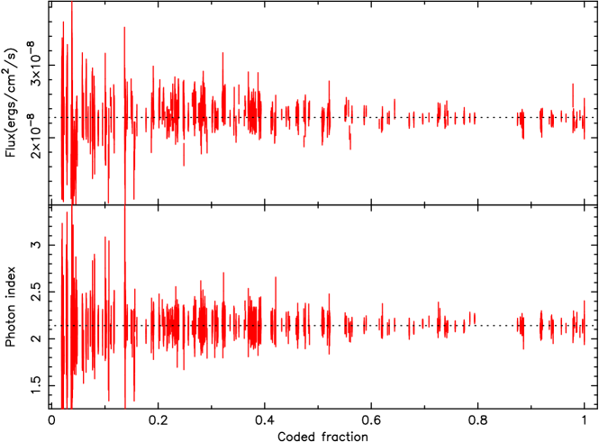
Figure 2: Crab flux in the 10-100 keV energy band (upper panel) and spectral photon index (lower panel) as a function of the coded fraction, as estimated with mask-weighting technique using celestial Crab coordinates. The horizontal dotted lines represent the best fit to the constant model (see table 3 for details).

	Detection Coordinates		Catalogue Coordinates
	FLUX
Coded fraction	Mean	rms	Mean	rms
$>$ 0	2.28E-08	7.7%	2.28E-08	8.1%
$>$ 0.1	2.28E-08	5.0%	2.28E-08	5.9%
	PHOTON INDEX
$>$ 0	2.14	0.09	2.14	0.11
$>$ 0.1	2.14	0.07	2.14	0.08

Table 3: Flux and power law statistic of Crab dataset. Fluxes in the 10-100 keV energy band are expressed in ergs cm^-2s^-1 units.

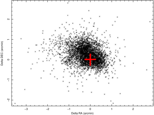
Figure 3: Dispersion of Crab detection coordinates around the nominal source position (red cross).We note that the coordinates dispersion is not perfectly centered on the Crab nominal position. Probably this is related to systematic image centroid shifts as a function of the position in the FOV (see BAT Digest pages), as well as to the distribution of the Crab detector coordinates in our dataset.

	Coded fraction $>$ 0	Coded fraction $>$ 0.1
$<1arcmin$	84.8%	90.9%
$<2arcmin$	98.6%	99.4%
$<3arcmin$	99.9%	100.0%

Table 4: Catalogue and detection coordinates percent difference.

Then, we repeated the mask weighting, as well as the spectral analysis, using as a starting point the source detection coordinates instead of the nominal ones. Results were found to be virtually undistinguishable (See Figure 4 and Table 3).

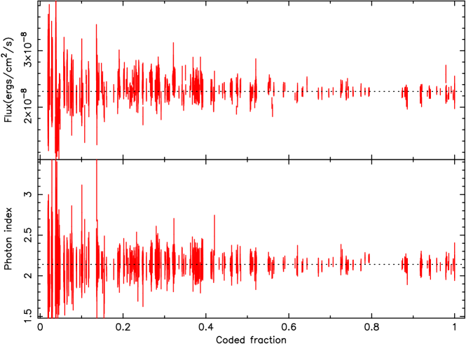
Figure 4: Crab flux in the 10-100 keV energy band (upper panel) and spectral photon index (lower panel) as a function of the coded fraction, as estimated with mask-weighting technique using Crab detection coordinates. The horizontal dotted lines represent the best fit to the constant model (see table 3 for details).

Figure 5 shows the flux difference as a function of the offset between the real Crab coordinate (in red) and those provided by the detection algorithm (in black). Considering the totality of the Crab data, we note that 96.0% of the detections lie within 3 arcmin from the source celestial coordinates and that their flux values differ by, at most, $\pm$5%. Considering only flux values extracted from observations with coded fraction greater than 0.1, the $\pm$5% threshold is met in 98.5% of the cases.

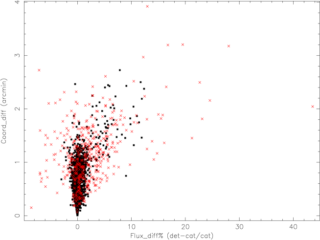
Figure 5: Flux difference using detection coordinates and nominal coordinates as a function of coordinate difference. Black squares represent the rows for which Crab was located at coded fraction greater than 0.1, whereas red crosses those for which the coded fraction was smaller or equal to 0.1 . We note that the use of detection coordinates induces a slight source flux overestimate which can be quantified in $\sim$0.5 %.

3.3 Results II: stacking multiple DPHs

DPH have a typical integration time of 5 minutes. A single-DPH analysis may be desirable in order to maximize time resolution. However, especially when dealing with faint sources, it may be important to increase statistics, at the expense of time resolution, by merging several DPHs. In general, different DPHs are collected with different mean satellite attitudes. Such a difference must be carefully checked before proceeding with the merging, since any offset may cause a partial loss in the reconstructed source flux. In order to quantify such an effect as a function of the pointing offset, we performed a simple test with the Crab. We started by selecting, among the data set described in section 3.1, DPHs where the Crab happened to be in three different FOV regions (at coded fraction 1, $\sim$0.5, $\sim$0.1). For each region, we selected a reference DPH together with a group of nearly co-aligned DPHs, having ROLL angles within 1 arcmin of the reference one, as well as pointing offsets (in R.A. and Dec.) within 7 arcmin of the reference one.

Then, each of the selected DPH rows was summed to the reference one, obtaining stacked DPH pairs, each being characterized by a “pointing offset” ranging from 0 to 7 arcmin. For each of such stacked pairs, we performed a spectral analysis and we extracted the Crab flux, to be compared with the one obtained from the reference DPH. Details on the handling of different attitude files for the construction and analysis of a pair are given in Appendix B.

The resulting flux-losses with respect to the reference DPH, as a function of the offset, for different coded fractions, are given in Table 5.

Although our investigation is far from complete, results suggest that significant flux losses ($>$ 5%) may occur, especially for target position at low coded fractions, when stacking different DPHs with a pointing offset larger than 2 arcmin. Thus, we decided conservatively to stack DPHs only if their pointings are within 1.5 arcmin.

Offset (arcmin)	Flux loss
Pcode = 1
1	0.1%
2	0.3%
3	1.9%
5	5.7%
7	11.1%
Pcode = 0.5
1	1.2%
2	3.6%
2.7	5.2%
4	19.4%
Pcode = 0.1
2	7.7%

Table 5: Crab flux loss for two DPH stacked as a function of the DPH pointing offset. Different positions of the Crab in the FOV have been considered.

4 Monitoring a strongly-variable source: the case of GRO J1655-40

Having assessed the overall correctness and reliability of our procedure on the bright Crab, we will proceed with the study of the microquasar GRO J1655-40, a source definitely fainter than the Crab and one known to be strongly variable, both in flux and in spectral shape.

GRO J1655-40 had a large outburst in 2005. Such an event started in the middle of February (it was discovered on February 17.99 during Galactic bulge scans with the RXTE/PCA instrument (Markwardt & Swank 2005)) and lasted for more than 9 months. In what follows we shall take advantage of a very large database serendipitously collected by the BAT instrument during the whole outburst event as well as of the systematic monitoring performed by the RXTE satellite.

This will allow us to compare our BAT results with quasi-simultaneous results obtained with the well calibrated instruments on-board RXTE. Such a cross-check will yield a very robust assessment of the capabilities of our analysis method as well as of the potentialities of BAT as a monitor for a (relatively) bright, strongly variable source.

4.1 BAT data analysis

All BAT observations covering the field of GRO J1655-40, collected between 2005/01/22 and 2005/11/11, were retrieved. The complete dataset includes 796 observations, for a total of 8724 DPHs, corresponding to $\sim$2.6 Ms observing time.

All the data analysis was performed by our automatic pipeline. As a first step, good data are selected, according to the prescription described in Appendix A.1. A total of 2080 ($\sim$24%) DPHs were discarded after data screening. Such a percentage is compatible with that found for the Crab dataset in section 3.2.

Next, well-aligned, contiguous DPHs are combined up to a maximum integration time of 1 hour. As a result, we obtained 1650 merged DPHs.

Then, from each data block, a spectrum is extracted with the mask-weighting technique, and the appropriate response matrix is produced.

An automatic spectral analysis is then carried out in XSPEC. After evaluating the source signal-to-noise, spectra with no signal (S/N=0)were discarded. This resulted in the rejection of 378 spectra ($\sim$ 23% of the total). Low S/N spectra (with source detection below $\sim 4\sigma$ level) are used to set an upper limit to the source flux. Contiguous, low-S/N spectra are summed, as well as their response matrices, in an attempt to increase the statistics, and the spectral analysis repeated on such combined spectra. High-S/N spectra are used for a complete spectral fit using a power law model.

A detailed description of the data analysis pipeline is given in Appendix A. The complete pipeline used for our study of GRO J1655-40 consists of steps 1, 2, 4, and 5 described there.

4.2 RXTE data analysis

RXTE monitored the whole outburst of GRO J1655-40 since its discovery (Markwardt & Swank 2005). The dataset is composed of 490 observations, performed between 2005-02-26 and 2005-11-11. Each observation has a typical integration time of $\sim$1.5 ks, for a total observing time of $\sim$664 ks.

Spectral data extracted from the complete dataset have been kindly made available to the community by the MIT group . Spectra for both source and background as well as response matrices and effective area files have been retrieved from their web site.

In order to ease a comparison of the results between different instruments, the same choices of energy range and spectral model were adopted. Thus, only data from the HEXTE instrument (operating in the 20-200 keV energy range) were used for the spectral fits. The spectral analysis was performed with an automatic pipeline based on the same algorithm adopted for BAT (as described in Appendix A). We discarded 53 low quality spectra, with S/N$<$3.5.

As a further step, data from the PCA instrument (operating in the 2-60 keV energy range) were used to extract a simple light curve (cts s^-1) in the soft (20-30 keV) energy range. An analogous light curve for the hard range (30-100 keV) was also extracted from HEXTE data and an hardness ratio plot was produced.

In addition, we downloaded public RXTE All Sky Monitor (ASM) data collected during the whole GRO J1655-40 outburst and extracted a count rate light curve in the 2-10 keV range.

4.3 Results

The complete light curve of the outburst of GRO J1655-40 as seen by BAT (in erg cm^-2 s^-1) is shown in Figure 6 (top panel). HEXTE measurements are also shown, to allow for a direct comparison. We plotted in the same figure the light curves extracted from the PCA data (count rate in 3-20 keV, central panel) and from the ASM data (count rate in 2-10 keV, bottom panel). Errors are at $1\sigma$ level.

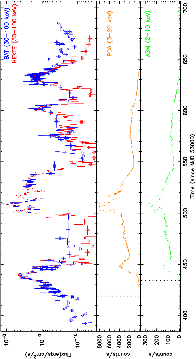
Figure 6: GRO J1655-40 complete 2005 outburst as seen from Swift/BAT and RXTE/HEXTE (upper panel), RXTE/PCA (central panel), and RXTE/ASM (lower panel). I n the upper panel, stars mark BAT and HEXTE points corresponding to averaged spectra. 3$\sigma$ upper limits are also plotted, marked by arrows. Vertical dotted bars in the central and lower panels represent the time of the first detection of the outburst obtained with PCA and ASM respectively.

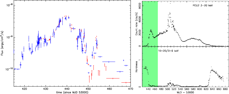
Figure 7: Left panel: zoom of the first part of the GRO J1655-40 outburst as seen by BAT (blue) and HEXTE (red) (symbols as in Figure 6). The right panel represents the PCA count rate and hardness ratio as obtained from the (http://tahti.mit.edu/opensource/1655/) web site. The green box highlights the time span covered in the left panel.

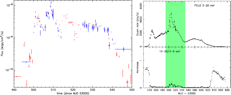
Figure 8: Zoom of the central part of the GRO J1655-40 outburst as seen by BAT (blue) and HEXTE (red).

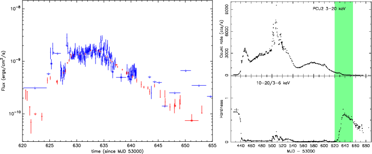
Figure 9: Zoom of the final part of the GRO J1655-40 outburst as seen by BAT (blue) and HEXTE (red).

Zooms of sections of the light-curve are shown in figures 7, 8 and 9, where the light-curves and hardness ratio plots obtained with the PCA instrument (taken from http://tahti.mit.edu/opensource/1655/) are also given. In spite of the different time coverage of such a strongly variable source, the agreement between the BAT and HEXTE light curves is remarkably good.

It is somewhat difficult to perform a direct quantitative comparison since BAT and HEXTE observations are not strictly simultaneous and the source shows a large variability on short timescales. Generally, BAT and HEXTE measurements appear to be fully consistent within errors. Considering time windows for which the BAT and HEXTE observations are frequent and close in time, a difference not larger than $\sim$10-15% is apparent when the source flux is above 1-2 $\times$10^-9 erg cm^-2s^-1, or $\sim 90$ mCrab. Generally, a good agreement (within errors) is found when the S/N in BAT spectra is greater than 4. The actual flux yielding such a S/N obviously depends on the position of the target within the FOV. Indeed, in one hour exposure, the $3\sigma$ sensitivity with our approach is $\sim 10-20$ mCrab for an on-axis source, while it is a factor $\sim 10$ worse at a coded fraction 0.2. Thus, if the target lies within the half-coded region, our approach yields significant spectral measurements (consistent with HEXTE) in the 30-100 keV range down to $(5-6)\times 10^{-10}$ erg cm^-2s^-1, or $\sim 50$ mCrab (see e.g. Fig 9, around MJD 53640). The study of sources fainter than $\sim 50$ mCrab would require a different and more complex approach.

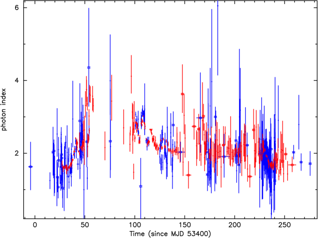
Figure 10: Spectral photon index evolution of the GRO J1655-40 outburst as obtained by fitting a power law independently to BAT (blue) and HEXTE (red) spectra. Errors are given at 1$\sigma$ level. Star labeled BAT and HEXTE points correspond to averaged spectra.

A good agreement between the power law photon index values as measured by BAT and HEXTE is also apparent in Figure 10. This is particularly evident if we consider the time intervals corresponding to the highest source flux (above $\sim$2 $\times$ 10^-9 ergs cm^-2 s^-1), as shown in Fig. 11, where BAT and HEXTE values agree to within $\sim$13% with no apparent correlation between spectral shape and flux discrepancy.

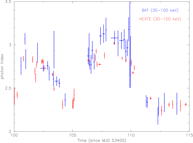
Figure 11: Zoom of figure 10 for the central part of the outburst.

Fig. 6 is a clear proof of the good capabilities of our method in order to extract flux and spectral informations for bright hard X-ray sources. BAT serendipitous coverage yielded a monitoring with a time coverage fully comparable to that obtained through a systematic campaign with RXTE. We note that BAT, simply owing to its good sensitivity over a very large FOV, caught the outburst since the very beginning, while the detection of the source activity by HEXTE and PCA was due to planned observational campaign of the Galactic center region (PCA Galactic bulge scans). Had GRO J1655-40 be located outside the galactic bulge region scanned by RXTE, its outburst would have been detected by ASM with $>$15 day delay with respect to BAT (see figure 7).

5 Summary and conclusions

We have developed and tested a procedure, based on public available Swift software tools, aimed at extracting flux and spectral information for bright hard X-ray sources from BAT “survey” data. Tests performed using a large sample of Crab data have shown that our pipeline, based on the mask-weighting technique, yields reliable measurements, both in spectral shape and in flux, over the whole BAT FOV. Using those results as a starting point, a more comprehensive test of our method was carried out on a fainter, strongly variable source such as GRO J1655-40. Its 9-month long outburst was systematically monitored with PCA and HEXTE instruments on board RXTE satellite and serendipitously observed by BAT. The cross-check performed by analysing indipendently the BAT and HEXTE spectra has shown a very good agreement between the two instruments when the source signal-to-noise in BAT spectrum is greater than 4 ($\sim$50 mCrab, for a target within the half coded region), confirming the reliability of our approach for using BAT as a hard X-ray monitor for bright sources. Combining such good performances with the huge BAT FOV, which covers each day $\sim$50% of the sky, one realizes the instrument’s potential to frequently monitor the temporal and spectral evolution of numerous bright, hard-X ray sources. As shown in section 4.3, BAT has been able to detect the beginning of the GRO J1655-40 outburst almost simultaneously with PCA instrument, which was luckily on target. Thus, while scanning the sky waiting for GRBs, BAT can be used both for detecting emission from hard X-ray transients and for monitoring the temporal and spectral evolution of known sources.

Appendix A Data analysis pipelines

In this section we provide a detailed description of the automatic pipelines used throughout this work. We divide the pipeline into different sections: 1) Preliminary data selection and preparation; 2) Imaging analysis; 3) mask weighting; 4) spectral analysis.

A.1 Preliminary data selection and preparation.

We describe here the prescription we used to select a good-quality, reliable dataset.

• First of all, we select data, collected in the desired time interval, with the target inside the BAT FOV. Data, including housekeeping and auxiliary files, may be searched and retrieved through the Swift data archive (see http://heasarc.gsfc.nasa.gov/cgi-bin/W3Browse/swift.pl).

• We correct DPH energy scale using gain offset maps. Gain offset files, stored among housekeeping files, are not supplied for each obs id. The most recent available file is selected for each observation, (the mean time between the file and the next is $\sim$3h). The ad-hoc tool baterebin is used to perform the correction.

• We reject bad datasets. Data filtering is performed using information stored both in housekeeping and attitude files:

  • Attitude information. Data for which the star tracker is not locked and the spacecraft is not in pointing mode are rejected.

  • Number of enabled detectors. To optimize imaging capabilities and detector performances, a minimum number of enabled detectors is required. DPH collected with less than 24000 enabled detectors are rejected.

  • Background noise. DPHs with anomalously high background noise may be identified by checking the total detector count rate. If such value exceeds 18000 counts s^-1 in the 14-190 keV energy band, data are discarded.

  • Avoidance angles and occultations. Data for which the angle between pointing and Earth limb is less than 30 degrees, or the spacecraft is in South Atlantic Anomaly (SAA) are discarded. Time intervals during which the source under study is occulted by Earth, Moon and Sun may be identified using the ad-hoc batoccultgti tool.

  • Overall data quality. DPHs for which data quality is nominal may be identified by checking appropriate flag stored in each DPH file.

  Each of the above criteria yields a Good Time Interval (GTI) table. The intersection of all such GTIs yields a table we used to screen for bad data. The resulting GTI is possibly unnecessarily restrictive. Often good data may be discarded because of a few seconds bad GTI intersection. In order to avoid such a problem, we added on both sides of each time interval a small allowance of 10% of the time interval. If such a value exceeds 10 seconds, we set the allowance to 10 s. Next, we checked all DPH times against resulting GTIs using the batbinevt tool, both for entire DPH and for a combination of DPH rows. Only the total intersected data will be considered for further analysis.

• We update attitude information. A new attitude file based on the median pointing direction, as evaluated considering only the observation GTI, is generated using the aspect tool.

A.2 Imaging analysis and source detection.

We give here details on the procedure we used to extract an energy resolved image of the sky and to search for the source of interest as well as for new ones.

• we create a Detector Plane Image (DPI). DPIs are obtained from DPH by adding, for each detector, the total counts recorded. Energy selections may be performed a priori in order to have energy-resolved DPIs. Such operations may be performed using the batbinevt tool.

• we generate a detector mask starting from the map of enabled/disabled detectors stored in the housekeeping files. As for the case of gain offset files, detector masks are not supplied for each observation. They are supposed not to change rapidly, so we used the nearest available file. Hot pixels are then searched and identified using the ad-hoc task bathotpix. A bad pixel map is obtained, and it is combined to the original map to produce the final detector mask.

• we create a background map for each DPI, not accounting for sources inside the FOV, using the batclean tool, the detector mask, and the default background model.

• we built the sky image. Each DPI was deconvolved from the coded aperture mask and translated to a background-subtracted image of the sky (including all the sources within the instrument FOV) with the ad-hoc task batfftimage, using the background map, the corrected attitude file and the merged detector mask.

• we create a coded fraction map. A map of the sky coded fraction across the instrument FOV was obtained using the batfftimage tool using the same inputs as above. Values of 1 are applied to fully coded regions, 0 to the edges of FOV.

• we run the source detection algorithm. We used the ad-hoc task batcelldetect to perform a source detection on the resulting sky images. A list of sources above a desired signal-to-noise threshold (we adopted 3.8) and a partially-coded fraction threshold (we adopted 0.001) is generated, including sky and image coordinates, signal-to-noise, count rate, coded fraction and other useful pieces of information for each source.

The procedure outlined above may be run either on a single-row DPH, or on a merged DPH.

A.3 Mask-weighting technique.

We describe here the procedure we used to extract the source spectrum using the mask weighting approach, as well as to generate appropriate response matrix. The source coordinates must be known a priori (either from source detection, or from independent measurements). This section of our pipeline uses as input either a single-row DPH, or a merged DPH.

• We generate the weight map for the source under study for each DPH. The ad-hoc tool batmaskwtimg is used to this aim, using the detector mask as well as the corrected attitude files described above.

• We extract the source background-subtracted spectrum from each DPH. This is done with the batbinevt tool, using energy corrected, GTI-filtered DPH together with the corresponding weight map.

• We generate an ad-hoc response matrix response matrix (including effective area information) for each spectrum using the task batdrmgen.

• We add systematic error. The spectrum extracted as described above does not include systematic errors, which may be relevant at low energy ($<$25 keV). The batphasyserr tool may be used to add ad-hoc (as stored in the CALDB) systematics to each spectrum.

A.4 Spectral Analysis.

This section of the pipeline is devoted to the automatic spectral analysis of a source strongly variable both in flux and in spectral shape. We proceed as follows:

• Evaluation of the target signal-to-noise.
  As a first step, we estimate the source signal-to-noise for each spectrum. This is simply done by selecting a suitable spectral range, which has to be optimized on a case by case basis, and checking the source count rate together with its associated error. If the ratio between the count rate and the error is null or negative, the spectrum (and the corresponding DPH group) is discarded. If such ratio is positive, then further steps are performed.

• Initial guess of the spectral shape using hardness ratio which is required in order to optimize an automatic, “blind” spectral analysis. For the case of a strongly variable source, we used a hardness ratio criterion. Such an approach may allow to discriminate between different source states, and/or to identify the presence and relative contribution of different spectral components. The resulting hardness ratio values allow to choose the spectral model to be used to fit the source spectra, and/or to select an appropriate energy range to perform spectral analysis. GRO J1655-40 shows a strong, variable thermal component, dominating the source spectrum below 10 keV, while up to $\sim 100$ keV the spectrum is well reproduced by a power law ((Zhang et al. 1997); (Hynes et al. 1998)). Sometimes the thermal component yields a very significant (or even dominant) contribution up to more than 20 keV. In order to simplify the spectral analysis using a single-component model, the hardness ratio test was used to select the energy range minimizing the thermal contribution. In particular, we considered the hardness ratio between the 16-22 keV and 20-70 keV energy ranges. Spectra with a high count rate in the soft band are studied in 30-100 keV energy range, otherwise the 10-100 keV band is used.

• Evaluation of the source flux.
  Before running a complex spectral fit (also in view of the hardness ratio results), we perform a preliminary fit with a simplified model (reducing, e.g., the number of free spectral parameters) to get the source flux with its associated error. We used the flux/error ratio as a criterium to decide if the data quality warrant a deeper spectral model. In particular, a preliminary power law fit with a photon index fixed to -3 was performed and the source flux was evaluated. A flux/error ratio threshold of 4 was used to discriminate between low and high S/N spectra.

• Low S/N spectra.
  Spectra with poor S/N are used to set an upper limit to the source emission using the simplified model.

• Further analysis of low S/N spectra.
  We made an attempt to recover spectral information, by summing low S/N spectra extracted from consecutive groups of DPHs, up to a maximum of 10 contiguous spectra. The corresponding response matrices are also combined. The resulting spectra are then analysed through the same steps of the automated pipeline.

• High S/N spectra.
  Spectra with an adequate S/N are studied in detail within Xspec. After spectral fitting, the best spectral parameters, as well as the source refined flux, are computed together with their uncertainties. In our case, a power law was used. The normalization was evaluated at 40 keV in order to minimize correlation with the photon index (see Ulrich-Demoulin & Molendi 1996).

Appendix B Attitude information for stacked DPHs

In order to understand the section dealing with the stacking of different DPH, focused on the maximum allowed misalignement between the observations, a brief explanation about the aspect tool, handling the attitude information on DPHs, is necessary. aspect calculates the mean pointing for a given attitude file as follows: the algorithm first creates a two-dimensional histogram of the amount of time spent at each RA and DEC, then selects the bin with the largest time and calculates the mean RA, DEC and ROLL angle of the spacecraft axes while RA and DEC angles were in this bin. The default binsize for such an histogram is 0.01 degs and usually a large fraction of the integration time of a DPH refers to a single bin of such size. This means that, if we stack two DPHs with an offset larger than 0.01 degs, the resulting pointing coordinates as obtained with aspect will be the same of the fraction of DPH accounting for the peak in the above described histogram. In the case of two histogram bins with the same amount of time, aspect calculates the mean of the relevant coordinates. If the offset is smaller than 0.01 degs (or than the selected binsize), aspect calculates the mean of the coordinates, as described above. Our approach was to leave fixed the default aspect binsize value and to choose, for each of the three coded fraction regions selected above, a reference single DPH’s row with 450 s exposure time: any other selected DPH’s row with the same exposure time was stacked on it.

In practice, considering offset up to few arcmin, the use of a larger aspect binsize does not change significantly the flux estimation of the source.