arXiv:0709.3791 YITP-07-57 OU-HET 586/2007 Moduli stabilization in 5D gauged supergravity
with universal hypermultiplet and boundary superpotentials

1 Introduction

Supersymmetric (SUSY) extension of the Randall-Sundrum (RS) model [1, 2, 3] provides an interesting setup for the physics beyond the standard model. For instance, localized wavefunctions in the extra dimension can be considered as a source of Yukawa hierarchy [4] as well as the large hierarchy between the weak and the Planck scales. The SUSY breaking sector can be sequestered from the visible sector in the extra dimension resulting in a flavor blind SUSY breaking patterns of the superparticle masses and couplings, i.e., anomaly mediation [5]. Besides, the application of the so-called AdS/CFT correspondence [6] to the SUSY RS model might provide a way to analyze perturbatively the four-dimensional (4D) strongly coupled theories.

On the other hand, the superstring theories would provide a unified framework of the standard model and gravity. It is known that a low energy effective theory of the strongly coupled heterotic string theory [7] can be described by 5D supergravity on an orbifold, which is sometimes referred to as the 5D heterotic M-theory [8]. Some three-brane solutions have been derived in such 5D model, which can be utilized to construct brane-world scenarios of our universe, where the visible sector and the hidden sector reside in different branes located at different orbifold fixed points.

All the above examples can be categorized into a unique theory, i.e., the 5D gauged supergravity, and share a common important subject, that is, an issue of moduli stabilization. 5D models have at least a radius modulus, i.e., the radion, whose vacuum value corresponds to the radius of the extra dimension. In 4D effective theory of 5D models, some couplings depend on the radius which is undetermined unless the radion is dynamically stabilized. If a 5D model is an effective theory of some higher-dimensional model, there might exist other moduli. These moduli fields including the radion form supermultiplets in the 4D effective theory if the compactification respects $N=1$ SUSY, and these multiplets can mediate SUSY breaking effects. Thus the moduli stabilization is one of the most important issues in the model building based on the higher-dimensional theory.

Several years ago, an interesting class of the moduli stabilization scheme was proposed by Kachru-Kallosh-Linde-Trivedi (KKLT) [9] based on the type IIB supergravity [10]. In such framework, light moduli are first stabilized at a SUSY preserving anti-de Sitter (AdS) minimum of the scalar potential. Then it is uplifted to a Minkowski minimum by a SUSY breaking vacuum energy generated in the hidden sector such as anti D-branes [9, 11], or dynamically generated F-terms [12, 13] and D-terms [14], which are well sequestered from the light moduli as well as the visible sector. This scenario overcomes, in a controllable manner, a big difficulty existing in supergravity/string compactifications [15], that is, a realization of the SUSY breaking Minkowski vacuum where all the moduli are stabilized, which is required from the observation of our universe.

Moreover, it has been shown that this kind of moduli stabilization procedures generically yields an interesting pattern of soft SUSY breaking terms in the visible sector, that is, the mirage mediation [11, 16, 17]. In the mirage mediation, the modulus-mediated contribution is comparable to that of the anomaly mediation. The low energy superparticle spectrum is quite different from the other mediation schemes such as the pure modulus mediation, the pure anomaly mediation and the gauge mediations. These would be distinguished by high-energy experiments and cosmological observations in future.

In this paper we study 5D gauged supergravity with a universal hypermultiplet whose isometry group is $SU(2,1)$. We consider various gaugings of the isometries and introduce some superpotential terms at the orbifold fixed points. Among eight independent isometries, we focus on three directions to gauge by the graviphoton. Thus the model we consider has three gauging parameters $(\alpha,\beta,\gamma)$ and includes both the SUSY RS model with an arbitrary bulk mass parameter for the hypermultiplet and 5D heterotic M-theory as different choices of the parameters. We investigate the vacuum structure of such models, especially the nature of moduli stabilization, assuming perturbative superpotential terms at the fixed points. Motivated by the KKLT moduli stabilization scheme, we also discuss the uplifting of SUSY AdS vacua in our models and the resultant SUSY breaking.

The following sections are arranged as follows. In Sec. 2, we review the $N=1$ off-shell description of 5D supergravity and see the representation of the isometries on the scalar manifold in such description. Then we derive the 4D effective action of a class of models obtained by gauging three independent isometries by the graviphoton with arbitrary superpotential terms at the orbifold fixed points. In Sec. 3, we study the moduli stabilization and the uplifting of the scalar potential in a case where the effective Kähler and superpotentials are expressed by analytic functions. In Sec. 4, we carry out a similar analysis in a model which corresponds to the generalized Luty-Sundrum model [18]. Sec. 5 is devoted to the summary. In Appendix, we show how to derive the isometry transformations in the on-shell description of 5D supergravity from the off-shell formulation.

2 4D effective action of 5D gauged supergravity

2.1 N=1 off-shell description of 5D supergravity action

In this paper we consider 5D gauged supergravity compactified on an orbifold $S^{1}/Z_{2}$ with a universal hypermultiplet and arbitrary superpotentials at the fixed points (or the boundaries) of the orbifold. The metric is written as

$$ds_{5}^{2}=e^{2\sigma(y)}g_{\mu\nu}dx^{\mu}dx^{\nu}-(e_{y}^{\;\;4}dy)^{2},$$ (2.1)

where $\sigma(y)$ is a warp factor. The off-diagonal components of the metric $g_{\mu y}$ is gauged away. We take the fundamental region of the orbifold as $0\leq y\leq\pi R$, where $R$ is a constant, and take the unit of $M_{5}=1$, where $M_{5}$ is the 5D Planck mass.

The off-shell description of 5D supergravity is quite useful for our purpose. It enables us to treat the localized terms at the orbifold boundaries independently from the bulk action. Furthermore as will be seen in the next subsection, the isometries of the scalar manifold, some of which are to be gauged, are linearly realized in the off-shell description. Therefore we start from 5D off-shell (conformal) supergravity developed by Ref. [19]-[22]. 5D superconformal multiplets relevant to our study are the Weyl multiplet $\mbox{\boldmath$E$}_{W}$, the vector multiplets $\mbox{\boldmath$V$}^{I}$ and the hypermultiplets $\mbox{\boldmath${\cal H}$}^{\hat{a}}$, where $I=0,1,2,\ldots,n_{V}$ and $\hat{a}=1,2,\ldots,n_{C}+n_{H}$. Here $n_{C}$, $n_{H}$ are the numbers of compensator and physical hypermultiplets, respectively. These 5D multiplets are decomposed into $N=1$ superconformal multiplets [22] as $\mbox{\boldmath$E$}_{W}=(E_{W},V_{E})$, $\mbox{\boldmath$V$}^{I}=(V^{I},\Sigma^{I})$ and $\mbox{\boldmath${\cal H}$}^{\hat{a}}=(\Phi^{2\hat{a}-1},\Phi^{2\hat{a}})$, where $E_{W}$ is the $N=1$ Weyl multiplet, $V_{E}$ is the $N=1$ general multiplet whose scalar component is $e_{y}^{\;\;4}$, $V^{I}$ is the $N=1$ vector multiplet, and $\Sigma^{I}$, $\Phi^{2\hat{a}-1}$, $\Phi^{2\hat{a}}$ are $N=1$ chiral multiplets.

The 5D supergravity action can be written in terms of these $N=1$ multiplets [23], in which $V_{E}$ has no kinetic term. After integrating $V_{E}$ out, the 5D action is expressed as [24, 25]

$${\cal L} = -3e^{2\sigma}\int d^{4}\theta\,{\cal N}^{1/3}({\cal V})\left\{d_{a}^{\ b}\bar{\Phi}^{b}(e^{-2igt_{I}V^{I}})^{a}_{\ c}\Phi^{c}\right\}^{2/3}$$ (2.2)

$$-e^{3\sigma}\bigg{[}\int d^{2}\theta\,\Phi^{a}d_{a}^{\ b}\rho_{bc}(\partial_{y}-2igt_{I}\Sigma^{I})^{c}_{\ d}\Phi^{d}+\textrm{h.c.}\bigg{]}$$

$$+\sum_{\vartheta=0,\pi}{\cal L}^{\vartheta}\,\delta(y-\vartheta R)+\cdots,$$

where $e^{2\sigma}$ is the warp factor of the background metric to be determined on-shell, $d_{a}^{\ b}={\rm diag}({\bf 1}_{2n_{C}},-{\bf 1}_{2n_{H}})$, $\rho_{ab}=i\sigma_{2}\otimes{\bf 1}_{n_{C}+n_{H}}$ and ${\cal N}({\cal V})$ is a cubic function defined by

$${\cal N}({\cal V})\equiv C_{IJK}{\cal V}^{I}{\cal V}^{J}{\cal V}^{K},$$ (2.3)

where $C_{IJK}$ is a real constant tensor which is completely symmetric for indices, and ${\cal V}^{I}\equiv-\partial_{y}V^{I}+\Sigma^{I}+\bar{\Sigma}^{I}$ is a gauge-invariant quantity. The ellipsis in (2.2) denotes the vector multiplet part. The boundary Lagrangian ${\cal L}^{\vartheta}$ can be introduced independently of the bulk action. Note that (2.2) is a shorthand expression for the full supergravity action. We can always restore the full action by promoting the $d^{4}\theta$ and $d^{2}\theta$ integrals to the $D$- and $F$-term formulae of $N=1$ conformal supergravity formulation [26], which are compactly listed in Appendix C of Ref. [22]. In the above expression of the 5D action, the hypermultiplet isometries are linearly realized. We can partially or fully gauge these isometries by the vector multiplets ${\mbox{\boldmath$V$}}^{I}=(V^{I},\Sigma^{I})$ with the generator $igt_{I}$.

2.2 Gauged supergravity with universal hypermultiplet

Now we consider the gauged supergravity with a single universal hypermultiplet spanning the manifold $SU(2,1)/SU(2)\times U(1)$. The universal hyperscalars are commonly denoted as $S$ and $\xi$, which are even and odd under the orbifold parity [27, 28]. The scalar manifold has an $SU(2,1)$ isometry group, which is nonlinearly realized in the on-shell description [27]. (See (A.6) in Appendix A, for example.) In the off-shell description (2.2), on the other hand, it is linearly realized. This greatly simplifies the analysis. The situation we consider is realized by taking $(n_{C},n_{H})=(2,1)$. Then the bulk action in (2.2) has a $U(2,1)$ symmetry. Since the superconformal gauge-fixing conditions can eliminate only one compensator multiplet, we introduce a nondynamical (auxiliary) Abelian vector multiplet ${\mbox{\boldmath$V$}}_{T}=(V_{T},\Sigma_{T})$ to eliminate the other compensator multiplet. We gauge the overall $U(1)$ subgroup of the symmetry group $U(2,1)$, which we refer to as $U(1)_{T}$, by ${\mbox{\boldmath$V$}}_{T}$ [21]. Namely the charges of the hypermultiplets for this gauging are assigned as $igt_{T}=\sigma_{3}\otimes{\mbox{\boldmath$1$}}_{2+n_{H}}$. As a result the symmetry group is reduced to $SU(2,1)$ after eliminating the nondynamical vector multiplet ${\mbox{\boldmath$V$}}_{T}$. The $Z_{2}$-parities and the $U(1)_{T}$ charges of the $N=1$ multiplets are listed in Table. 1.

	$V^{I^{\prime}}$	$\Sigma^{I^{\prime}}$	$V^{I^{\prime\prime}}$	$\Sigma^{I^{\prime\prime}}$	$V_{T}$	$\Sigma_{T}$	$\Phi^{1}$	$\Phi^{2}$	$\Phi^{3}$	$\Phi^{4}$	$\Phi^{5}$	$\Phi^{6}$
$Z_{2}$-parity	$-$	$+$	$+$	$-$	$+$	$-$	$-$	$+$	$+$	$-$	$+$	$-$
$U(1)_{T}$ charge	0	0	0	0	0	0	1	$-1$	1	$-1$	1	$-1$

Table 1: The orbifold parities and the $U(1)_{T}$ charges of $N=1$ multiplet. The indices run over $I^{\prime}=0,1,\cdots,n^{\prime}_{V}$; $I^{\prime\prime}=n^{\prime}_{V}+1,n^{\prime}_{V}+2,\cdots,n_{V}$; $\hat{a}=2,3,\cdots,n_{H}+2$.

Two compensator multiplets ${\mbox{\boldmath${\cal H}$}}^{1}=(\Phi^{1},\Phi^{2})$ and ${\mbox{\boldmath${\cal H}$}}^{2}=(\Phi^{3},\Phi^{4})$ must have the opposite $Z_{2}$-parities for consistency with the superconformal gauge-fixing. (See the appendix in Ref. [21].) For the vector multiplets, we divide the index $I$ into $(I^{\prime},I^{\prime\prime})$ so that $V^{I^{\prime}}$ and $V^{I^{\prime\prime}}$ are odd and even under the $Z_{2}$-parity respectively.

The following analyses are independent of the number of $Z_{2}$-even vector multiplets $n^{\prime\prime}_{V}$, and then we just choose $n^{\prime\prime}_{V}=0$ to simplify the discussion (i.e., $I=I^{\prime}$). The gauged supergravity is obtained by gauging some directions within the isometry group $SU(2,1)$ by ${\mbox{\boldmath$V$}}^{I^{\prime}}$. In this paper we restrict ourselves to the simple case $n^{\prime}_{V}=0$, where only the graviphoton takes part in the gauging of the isometries. Namely the function ${\cal N}$ defined in (2.3) is now

$${\cal N}({\cal V})=\left({\cal V}^{0}\right)^{3}.$$ (2.4)

The most general form of the gauging is parameterized by

$$igt_{I=0} = \sum_{i=1}^{8}\tilde{\alpha}_{i}\,T^{i}$$ (2.5)

acting on $(\Phi^{1},\Phi^{3},\Phi^{5})^{t}$ or $(\Phi^{2},\Phi^{4},\Phi^{6})^{t}$, where $T^{i}$ ($i=1,\ldots,8$) are $3\times 3$ matrix-valued generators of $SU(2,1)$ shown in Eq. (A.4). Here the real coefficients $\tilde{\alpha}_{i}$ determine the gauging direction. Since the graviphoton is $Z_{2}$-odd, the parameters $\tilde{\alpha}_{i}$ ($i=1,2,4,5$) are $Z_{2}$-even while the others are $Z_{2}$-odd and have kink profiles for $y$. In the following, we consider a case that $\tilde{\alpha}_{i}$ are parameterized by three parameters ($\alpha,\beta,\gamma$) as

$$\tilde{\alpha}_{3}\!\!\! =\!\!\! 2\beta,\qquad\tilde{\alpha}_{6}=\alpha,\qquad\tilde{\alpha}_{8}=\alpha+\beta+\gamma,$$

$$\tilde{\alpha}_{i}\!\!\! =\!\!\! 0.\;\;\;\;\;(i\neq 3,6,8)$$ (2.6)

This class of models contain the following interesting models as special limits of the gauge parameters. In the limit of $\beta,\gamma\to 0$, this model is reduced to the 5D effective theory of heterotic M-theory, which is derived in Ref. [8] on-shell. As shown in Ref. [8], it has a linearly warped BPS background geometry given by

$$ds^{2} = (A+2\alpha y)^{1/6}dx^{2}-dy^{2},$$ (2.7)

where $A$ is a constant. In this case, the gauge parameter $\alpha$ is related to a flux, that is, a curvature four-form integrated over a four-cycle $C_{4}$ of the Calabi-Yau manifold,

$$\alpha \propto \int_{C_{4}}\,{\rm tr}\,R\wedge R.$$ (2.8)

If we turn on the $\beta$-gauging, the background metric (2.7) becomes

$$ds^{2}=e^{-2\beta y}(A+2\alpha y)^{1/6}dx^{2}-dy^{2},$$ (2.9)

and the model has an exponentially warped geometry. Especially it is reduced to the SUSY RS model [2, 3, 28] when $\alpha=0$. This means that the $\beta$-gauging induces a negative cosmological constant in the bulk, which leads to the AdS curvature $k=\beta$. We can see from the 5D action that it also induces the bulk mass $m=3\beta/2$ for the physical hypermultiplet. By introducing the $\gamma$-gauging to this case, the parameters $k$ and $m$ become independent and are given by

$$k = \beta-\frac{\gamma}{3},\qquad m\ =\ \frac{3}{2}(\beta+\gamma).$$ (2.10)

Note that these relations hold only when $\alpha=0$. If we turn on the $\alpha$-gauging, the model deviates from the SUSY RS model, and the above relations are modified to more complicated ones.

Thus the $(\alpha,\beta,\gamma)$-gauging model, which we refer to as the hybrid model in this paper, can be regarded as a hybrid formulation of the SUSY RS model and the 5D heterotic M-theory. Although we have gauged only three directions among eight isometries within $SU(2,1)$, this $(\alpha,\beta,\gamma)$-gauging model contains most of important structures in the gauged supergravity with a universal hypermultiplet because both the linear and the exponential warp factors can be realized just by taking different limit of the the gauge parameters. The other gauge parameters in Eq. (2.5) generate a similar warping such as $\sinh(y)$ or $\cosh(y)$ which are just combinations of the exponential factors.

Therefore, in the following, we study the $(\alpha,\beta,\gamma)$-gauging model in detail with boundary induced superpotentials. Since the boundary Lagrangian ${\cal L}^{\vartheta}$ must be invariant for $U(1)_{T}$, it is written as

$${\cal L}^{\vartheta}=e^{3\sigma}\left[\int d^{2}\theta\;\Phi^{2}\Phi^{3}P_{\vartheta}(Q)+{\rm h.c.}\right],$$ (2.11)

where $P_{\vartheta}(Q)$ ($\vartheta=0,\pi$) are the boundary superpotentials. The induced chiral multiplet $Q$ has zero Weyl weight and is neutral for $U(1)_{T}$. Thus it is identified as

$$Q=\frac{\Phi^{5}}{\Phi^{3}}.$$ (2.12)

Note that only $Z_{2}$-even multiplets can appear in ${\cal L}^{\vartheta}$.

2.3 4D effective action

Now we derive the 4D effective theory for the $(\alpha,\beta,\gamma)$-gauging with superpotentials $P_{\vartheta}$ at the orbifold fixed points. For this purpose, we adopt the off-shell dimensional reduction proposed by Refs. [24, 25], which are based on the $N=1$ superspace description [23] of the 5D off-shell supergravity and developed in subsequent studies [30]. This method enables us to derive the 4D off-shell effective action directly from the 5D off-shell supergravity action keeping the $N=1$ off-shell structure. The procedure is straightforward. We start from the $N=1$ off-shell description of 5D action (2.2) with (2.11). After some gauge transformation, we drop kinetic terms for $Z_{2}$-odd multiplets because they are negligible in low energies. Then those multiplets play a role of the Lagrange multipliers and their equations of motion extract zero-modes from the $Z_{2}$-even multiplets. Note that only the $Z_{2}$-even multiplets have zero-modes that appear in the effective theory.

In our model the $Z_{2}$-even multiplets are $\Sigma^{0}$, $\Phi^{2}$, $\Phi^{3}$ and $\Phi^{5}$. Due to the $U(1)_{T}$-invariance, they appear in the action only through the combinations of $\Sigma^{0}$, $\Phi^{2}\Phi^{3}$ and $\Phi^{5}/\Phi^{3}$ which carry the zero-modes, the radion multiplet $T$, 4D chiral compensator $\phi$ and the matter multiplet $H$, respectively. Following the procedure of Ref. [24, 25], we obtain the 4D effective action as

$$S_{\rm eff} = -3\int d^{4}\theta\,|\phi|^{2}e^{-K/3}+\left\{\int d^{2}\theta\,\phi^{3}W+\textrm{h.c.}\right\},$$ (2.13)

where the Kähler potential $K$ and the superpotential $W$ are given by

$$K = -3\ln\int^{\pi{\rm Re}\,T}_{0}dt\,e^{-2\beta t}\bigg{\{}\cosh\left(2t\sqrt{\gamma^{2}-2\alpha\gamma}\right)\,(1-|H|^{2})$$ (2.14)

$$\qquad+\sinh\left(2t\sqrt{\gamma^{2}-2\alpha\gamma}\right)\,\frac{(\alpha+\gamma)(1+|H|^{2})+\alpha(H+\bar{H})}{\sqrt{\gamma^{2}-2\alpha\gamma}}\bigg{\}}^{\frac{1}{3}},$$

$$W = \frac{1}{4}\sum_{\vartheta=0,\pi}e^{-3\vartheta\beta T}\left\{c_{\vartheta}+(\alpha+\gamma)s_{\vartheta}+\alpha s_{\vartheta}H\right\}P_{\vartheta}(H_{\vartheta}).$$ (2.15)

Here, $H_{\vartheta}$ and $(c_{\vartheta},s_{\vartheta})$ are defined as

$$H_{\vartheta} \equiv \frac{-\alpha s_{\vartheta}+\left(c_{\vartheta}-(\alpha+\gamma)s_{\vartheta}\right)H}{c_{\vartheta}+(\alpha+\gamma)s_{\vartheta}+\alpha s_{\vartheta}H},$$ (2.16)

$$c_{\vartheta} \equiv \cosh\left(\vartheta T\sqrt{\gamma^{2}-2\alpha\gamma}\right),\qquad s_{\vartheta}\ \equiv\ \frac{\sinh\left(\vartheta T\sqrt{\gamma^{2}-2\alpha\gamma}\right)}{\sqrt{\gamma^{2}-2\alpha\gamma}}.$$ (2.17)

As the boundary superpotentials $P_{\vartheta}(Q)$ in (2.11), we consider the following polynomials.

$$P_{\vartheta}(Q)=\sum_{n\geq 0}w_{\vartheta}^{(n)}Q^{n},$$ (2.18)

where $w_{\vartheta}^{(n)}$ ($n=0,1,2,\ldots$) are constants.

There are two simple cases to analyse. When $\gamma=0$, the Kähler potential $K$ can be expressed by an analytic function. When $\alpha=0$, on the other hand, the superpotential $W$ is reduced to a simple form, i.e., a polynomial for $H$. Thus we will discuss these two cases in detail in the next two sections.

3 Moduli stabilization in hybrid model ($\gamma=0$)

In the case that $\gamma=0$, the $t$-integration in the Kähler potential (2.14) can be carried out analytically. Such analytic expression allows us to study more about the 4D effective theory of the above hybrid model. In this section, we analyze the vacuum structure of the $(\alpha,\beta)$-gauging model assuming, for simplicity and concreteness, the boundary superpotentials consist of only constant and tadpole terms for the universal hypermultiplet, i.e., $w_{\vartheta}^{(n)}=0$ for $n\geq 2$ in (2.18).

After a Kähler transformation (which is equivalent to a rescaling of the chiral compensator $\phi$), the Kähler potential (2.14) and the superpotential (2.15) are expressed as

$$K\!\!\! =\!\!\! -3\ln\left\{\frac{1}{2\alpha}{\cal F}(S_{0},S_{\pi})\right\},$$

$$W\!\!\! =\!\!\! e^{-\frac{3}{2}qS_{0}}(a_{0}+b_{0}S_{0})-e^{-\frac{3}{2}qS_{\pi}}(a_{\pi}+b_{\pi}S_{\pi}).$$ (3.1)

where $q=\beta/\alpha$ and

$${\cal F}(S_{0},S_{\pi})\equiv q^{-4/3}\left\{\Gamma\left(\frac{4}{3},q{\rm Re}\,S_{0}\right)-\Gamma\left(\frac{4}{3},q{\rm Re}\,S_{\pi}\right)\right\}.$$ (3.2)

Here, $\Gamma(a,x)=\int_{x}^{\infty}dt\,t^{a-1}e^{-t}$ is the incomplete gamma function, and the chiral multiplets $S_{\vartheta}$ are defined as

$$S_{0}\equiv\ \frac{1-H}{1+H},\qquad S_{\pi}\equiv S_{0}+2\pi\alpha T.$$ (3.3)

The parameters $a_{\vartheta}$ and $b_{\vartheta}$ in the superpotential are given by linear combinations of the constants in the boundary superpotentials (2.18) as

$$a_{\vartheta}\!\!\! \equiv\!\!\! \frac{1}{8}\left(w_{\vartheta}^{(0)}+w_{\vartheta}^{(1)}\right),\;\;\;\;\;b_{\vartheta}\equiv\frac{1}{8}\left(w_{\vartheta}^{(0)}-w_{\vartheta}^{(1)}\right),\;\;\;\;\;(\vartheta=0,\pi).$$ (3.4)

The scalar component of $S_{0}$ defined in (3.3) corresponds to a zero-mode for the $Z_{2}$-even 5D scalar $S$ in the notation of Refs. [27, 28].

For given $K$ and $W$, the scalar potential $V$ is calculated by the formula,

$$V=e^{K}\left\{K^{X\bar{Y}}D_{X}WD_{\bar{Y}}\bar{W}-3\left|W\right|^{2}\right\},$$ (3.5)

where $D_{X}W\equiv W_{X}+K_{X}W$, and $X,Y$ run over all chiral multiplets. Note that the scalar potential (3.5) is that in the Einstein frame, which corresponds to a gauge where the chiral compensator scalar is fixed as

$$\phi=e^{K/6}.$$ (3.6)

Here and henceforth, we take the unit of the 4D Planck mass, i.e., $M_{\rm Pl}=1$. (In the previous section, we took the unit of the 5D Planck mass.)

In our model, $V$ is calculated as

$$V\!\!\! =\!\!\! \frac{-8\alpha^{3}}{{\cal F}(S_{0},S_{\pi})^{2}}\left[\left\{\frac{{\cal F}(S_{0},S_{\pi})}{3}+\frac{({\rm Re}\,S_{0})^{4/3}e^{-q{\rm Re}\,S_{0}}}{1-3q{\rm Re}\,S_{0}}-\frac{({\rm Re}\,S_{\pi})^{4/3}e^{-q{\rm Re}\,S_{\pi}}}{1-3q{\rm Re}\,S_{\pi}}\right\}^{-1}\right.$$ (3.7)

$$\hskip 71.13188pt\times\left|e^{-\frac{3}{2}qS_{0}}\frac{a_{0}-b_{0}\bar{S}_{0}}{1-3q{\rm Re}\,S_{0}}-e^{-\frac{3}{2}qS_{\pi}}\frac{a_{\pi}-b_{\pi}\bar{S}_{\pi}}{1-3q{\rm Re}\,S_{\pi}}\right|^{2}$$

$$\hskip 71.13188pt\left.-4\left\{({\rm Re}\,S_{0})^{2/3}e^{-2q{\rm Re}\,S_{0}}\frac{\left|b_{0}-\frac{3}{2}q(a_{0}+b_{0}S_{0})\right|^{2}}{1-3q{\rm Re}\,S_{0}}\right.\right.$$

$$\left.\left.\hskip 99.58464pt-({\rm Re}\,S_{\pi})^{2/3}e^{-2q{\rm Re}\,S_{\pi}}\frac{\left|b_{\pi}-\frac{3}{2}q(a_{\pi}+b_{\pi}S_{\pi})\right|^{2}}{1-3q{\rm Re}\,S_{\pi}}\right\}\right].$$

In this paper we use the same symbols for the scalar fields as the chiral multiplets they belong to.

3.1 Heterotic M-theory limit (pure $\alpha$-gauging)

In the limit $\beta\to 0$, Eq.(3.1) becomes

$$K\!\!\! =\!\!\! -3\ln\left[\frac{3}{8\alpha}\left\{({\rm Re}\,S_{\pi})^{4/3}-({\rm Re}\,S_{0})^{4/3}\right\}\right],$$

$$W\!\!\! =\!\!\! b_{0}\left\{C+S_{0}-rS_{\pi}\right\},$$ (3.8)

where

$$C\equiv\frac{a_{0}-a_{\pi}}{b_{0}},\qquad r\equiv\frac{b_{\pi}}{b_{0}}.$$ (3.9)

The above Kähler potential reproduces the known result, i.e., the 4D effective Kähler potential of the heterotic M-theory [31] when ${\rm Re}\,S_{0}\gg\pi\alpha{\rm Re}\,T$ as pointed out in Ref. [24]. The superpotential $W$ originates from the boundary superpotentials (2.18). In this case, the vacuum values of $S_{0}$, $S_{\pi}$ and ${\rm Re}\,T$ determine the Calabi-Yau volume at $y=0,\pi R$ and the radius of the compact 11th dimension, respectively. Here we assume that $\alpha>0$, then the scalar fields have to satisfy ${\rm Re}\,S_{\pi}>{\rm Re}\,S_{0}>0$ in order for them to have the physical interpretation as the volumes.

The scalar potential (3.7) is now reduced to

$$V=\left(\frac{8\alpha}{3}\right)^{3}\left|b_{0}\right|^{2}\left\{\frac{\left|C-\bar{S}_{0}+r\bar{S}_{\pi}\right|^{2}}{\left\{({\rm Re}\,S_{\pi})^{4/3}-({\rm Re}\,S_{0})^{4/3}\right\}^{3}}-3\frac{\left|r\right|^{2}({\rm Re}\,S_{\pi})^{2/3}-({\rm Re}\,S_{0})^{2/3}}{\left\{({\rm Re}\,S_{\pi})^{4/3}-({\rm Re}\,S_{0})^{4/3}\right\}^{2}}\right\}.$$ (3.10)

From the SUSY preserving conditions: $D_{S_{0}}W=D_{S_{\pi}}W=0$, we obtain

$${\rm Re}\,S_{\pi}\!\!\! =\!\!\! r^{3}{\rm Re}\,S_{0}.$$

$$2({\rm Re}\,S_{0})^{1/3}\left(C+S_{0}-rS_{\pi}\right)\!\!\! =\!\!\! ({\rm Re}\,S_{0})^{4/3}-({\rm Re}\,S_{\pi})^{4/3}.$$ (3.11)

The first equation indicates that SUSY point exists only when $r^{3}$ is real and positive. Thus we assume that $r$ is real positive in the following. Solving (3.11), we find a SUSY point,

$$({\rm Re}\,S_{0},{\rm Re}\,S_{\pi})\!\!\! =\!\!\! \left(\frac{2C_{R}}{r^{4}-1},\frac{2C_{R}r^{3}}{r^{4}-1}\right),$$ (3.12)

$$C_{I}+{\rm Im}\,S_{0}-r{\rm Im}\,S_{\pi}\!\!\! =\!\!\! 0,$$ (3.13)

where

$$C\equiv C_{R}+iC_{I}.$$ (3.14)

Since the scalars must satisfy ${\rm Re}\,S_{\pi}>{\rm Re}\,S_{0}>0$, this point is in the physical region only when $C_{R}>0$ and $r>1$. We focus on this parameter region. From Eq. (3.13), we find a flat direction in an imaginary direction of $S_{\vartheta}$. The superpotential takes the following value at the SUSY point.

$$W=-b_{0}C_{R}.$$ (3.15)

Thus from (3.5), the vacuum energy is negative at this SUSY point, that is, the geometry is AdS₄. By evaluating the second derivatives of the potential (3.10), we can see that this SUSY point is a saddle point. Here we should note that SUSY points are always stable in a sense that they satisfy the Breitenlohner-Freedman bound [32]. As will be done in Sect. 3.4, we will uplift the negative vacuum energy of the SUSY AdS vacuum by a SUSY breaking vacuum energy in the hidden sector in order to obtain a SUSY breaking Minkowski vacuum. In general a SUSY saddle point remains to be a saddle point after the uplifting unless the uplifting potential is steep, and such saddle point after the uplifting is not stable any more. So we would like to look for a local minimum of the potential which is expected to be stable after the uplifting.

When $r\gg 1$, there is another stationary point,

$$({\rm Re}\,S_{0},{\rm Re}\,S_{\pi})=\left(\frac{16C_{R}}{r^{4}},\frac{2C_{R}}{r}\right)\left\{1+{\cal O}\left(\frac{1}{r}\right)\right\},$$ (3.16)

along the direction (3.13). In contrast to the previous point (3.12), this point is a local minimum except for the flat direction (3.13). At this point,

$$D_{S_{0}}W\!\!\! =\!\!\! -b_{0},\;\;\;\;\;D_{S_{\pi}}W=b_{0}\times{\cal O}\left(\frac{1}{r}\right),\;\;\;\;\;W=-b_{0}C_{R}.$$ (3.17)

Thus this is a SUSY breaking AdS₄ vacuum.

3.2 Randall-Sundrum limit (pure $\beta$-gauging)

In the limit $\alpha\to 0$, the Kähler and the superpotentials (3.1) become

$$K\!\!\! =\!\!\! -3\ln\left(\frac{1-\left|\Omega\right|^{2}}{2\beta}\right)-\ln\left({\rm Re}\,S_{0}\right),$$

$$W\!\!\! =\!\!\! (a_{0}+b_{0}S_{0})-(a_{\pi}+b_{\pi}S_{0})\Omega^{3},$$ (3.18)

where $\Omega\equiv e^{-\beta\pi T}$ is a warp factor superfield. The above $K$ reproduces the radion Kähler potential of the SUSY RS model [18]. In the following, we assume $\beta>0$. Then the scalar fields must satisfy ${\rm Re}\,S_{0}>0$ and $\left|\Omega\right|<1$. Although $H$ is more conventional than $S_{0}$ for the SUSY RS model, we use $S_{0}$ as a matter chiral multiplet because we will interpolate this model and the Heterotic M-theory limit ($\alpha\neq 0$, $\beta\to 0$). We can always translate $S_{0}$ to $H$ by the relation (3.3).

In this limit, the scalar potential (3.7) is reduced to

$$V\!\!\! =\!\!\! \frac{8\beta^{3}}{(1-\left|\Omega\right|^{2})^{2}{\rm Re}\,S_{0}}\bigg{\{}\frac{\left|(a_{0}-a_{\pi}\Omega^{3})-\bar{S}_{0}(b_{0}-b_{\pi}\Omega^{3})\right|^{2}}{1-\left|\Omega\right|^{2}}$$ (3.19)

$$\qquad\qquad\qquad\qquad-3\left(\left|a_{0}+b_{0}S_{0}\right|^{2}-\left|\Omega\right|^{4}\left|a_{\pi}+b_{\pi}S_{0}\right|^{2}\right)\bigg{\}}.$$

From the SUSY conditions: $D_{S_{0}}W=D_{\Omega}W=0$, we obtain

$$\left(a_{0}-a_{\pi}\Omega^{3}\right)\left(\bar{b}_{0}-\bar{b}_{\pi}\frac{\bar{\Omega}^{2}}{\Omega}\right)+\left(b_{0}-b_{\pi}\Omega^{3}\right)\left(\bar{a}_{0}-\bar{a}_{\pi}\frac{\bar{\Omega}^{2}}{\Omega}\right)=0.$$ (3.20)

In the case that $a_{0}b_{\pi}-b_{0}a_{\pi}\neq 0$, we find a SUSY solution as

$$S_{0}=\frac{\bar{a}_{0}-\bar{a}_{\pi}\bar{\Omega}^{3}}{\bar{b}_{0}-\bar{b}_{\pi}\bar{\Omega}^{3}}=-\frac{a_{0}-a_{\pi}(\Omega^{2}/\bar{\Omega})}{b_{0}-b_{\pi}(\Omega^{2}/\bar{\Omega})},$$ (3.21)

where $\Omega$ is a solution of Eq. (3.20).

On the other hand, in the case that $a_{0}b_{\pi}-b_{0}a_{\pi}=0$, that is,

$$(a_{0},a_{\pi}) = c\,(b_{0},b_{\pi}),\;\;\;\;\;\left(\mbox{or }(w_{0}^{(0)},w_{\pi}^{(0)})=\frac{c+1}{c-1}(w_{0}^{(1)},w_{\pi}^{(1)})\right)$$ (3.22)

where $c$ is a constant, the relation (3.20) is rewritten as

$$({\rm Re}\,c)(1-r\Omega^{3})\left(1-\bar{r}\frac{\bar{\Omega}^{2}}{\Omega}\right)=0,$$ (3.23)

where $r\equiv b_{\pi}/b_{0}$, and the superpotential in this case is found as

$$W=b_{0}(c+S_{0})(1-r\Omega^{3}).$$ (3.24)

For ${\rm Re}\,c<0$, the SUSY point is found as

$$(S_{0},\Omega)=\left(-c,\,r^{-1/3}\right).$$ (3.25)

At this point, $W=0$ and thus the vacuum energy vanishes, resulting a local Minkowski minimum. This corresponds to the SUSY Minkowski vacuum discussed in Ref. [34], in which the boundary superpotentials (2.18) consist of only the tadpole terms, i.e., $w_{\vartheta}^{(0)}=0$ (or $c=-1$.)

For ${\rm Re}\,c>0$, the SUSY solution is found as

$$(S_{0},\Omega)=\left(\bar{c},\,\left|r\right|^{-4/3}\bar{r}^{1/3}\right),$$ (3.26)

where the superpotential does not vanish at this point,

$$W=2b_{0}({\rm Re}\,c)\left(1-\frac{1}{\left|r\right|^{2}}\right)\neq 0.$$ (3.27)

This means that the vacuum energy is negative and the geometry becomes AdS₄. This SUSY solution is a saddle point.

In either case, the SUSY point exists in the region ${\rm Re}\,S_{0}>0$ and $\left|\Omega\right|<1$ only when $\left|r\right|>1$. For ${\rm Re}\,c=0$, $S=-c=\bar{c}$ and $\Omega$ is undetermined.

In the following, we focus on the case (3.22) where the scalar potential (3.19) is simplified as

$$V=\frac{8\beta^{3}\left|b_{0}\right|^{2}}{(1-\left|\Omega\right|^{2})^{2}{\rm Re}\,S_{0}}\left\{\frac{\left|c-\bar{S}_{0}\right|^{2}\left|1-r\Omega^{3}\right|^{2}}{1-\left|\Omega\right|^{2}}-3\left|c+S_{0}\right|^{2}\left(1-\left|r\right|^{2}\left|\Omega\right|^{4}\right)\right\}.$$ (3.28)

Here we have decomposed the complex scalars and the parameters into real ones as

$$S_{0}=s+i\sigma,\;\;\;\;\;\Omega=\omega e^{i\varphi},\;\;\;\;\;r=\rho e^{i\zeta},\;\;\;\;\;c=c_{R}+ic_{I}.$$ (3.29)

From the stationary conditions for $\sigma$ and $\varphi$, we obtain

$$c_{I}+\sigma=0,\;\;\;\;\;\sin(\zeta+3\varphi)=0.$$ (3.30)

Focusing on the SUSY local minimum (3.25), we calculate the mass eigenvalues. Evaluating the second derivatives of the scalar potential (3.28), we can see that the four real scalars $(s,\omega,\sigma,\varphi)$ do not mix with each other. Then after normalizing them canonically, the mass eigenvalues are found as

$$m_{s}^{2}\!\!\! =\!\!\! m_{\omega}^{2}=96\beta^{3}\left|b_{0}\right|^{2}\left|c_{R}\right|\frac{\rho^{4/3}(1+\rho^{-2/3})^{2}}{1-\rho^{-2/3}},$$

$$m_{\sigma}^{2}\!\!\! =\!\!\! m_{\varphi}^{2}=48\beta^{3}\left|b_{0}\right|^{2}\left|c_{R}\right|\frac{\rho^{2/3}}{1-\rho^{-2/3}}.$$ (3.31)

We have assumed $c_{R}<0$ and $\rho>1$.

3.3 Interpolation

In the previous subsections, we analyzed in detail the vacuum structures in the two typical limits of the hybrid model, i.e., the heterotic M-theory limit (pure $\alpha$-gauging) and the SUSY RS limit (pure $\beta$-gauging). In this subsection, we study intermediate regions of the hybrid model. We assume that the parameters satisfy the relation (3.22) with $c_{R}\equiv{\rm Re}\,c<0$ for simplicity of the analysis.

3.3.1 Numerical result

First we show some numerical results. We focus on the SUSY preserving points (3.12) in the pure $\alpha$-gauging and (3.25) in the pure $\beta$-gauging, and numerically interpolate these stationary points in the intermediate region, where both $\alpha$ and $\beta$ are nonvanishing.

Figure 1: The gravitino mass on the $({\rm Re}\,S,{\rm Re}\,T)$-plane. We vary the parameter $\alpha$ from $100$ (left end-point) to $0.1$ (right end-point) by fixing $\beta=1$, $c=-40$, $r=10^{5}$ and $b_{0}=10^{-14}$. All the mass scales are measured in the unit $M_{\rm Pl}=1$.

Fig. 1 plots the gravitino mass and the position of the SUSY point on the $({\rm Re}\,S,{\rm Re}\,T)$ plane for various values of $\alpha$ with the other parameters fixed. The left end-point of the curve corresponds to $\alpha=100$ (near the M-theory limit) and the other end-point corresponds to $\alpha=0.1$ (near the SUSY RS limit). The curve on the $({\rm Re}\,S,{\rm Re}\,T)$ plane represents the projection on that plane. Since the vacuum energy at the SUSY point $V_{\rm SUSY}$ is related to the gravitino mass $m_{3/2}=e^{K/2}\left|W\right|$ through $V_{\rm SUSY}=-3m_{3/2}^{2}$, we can see from Fig. 1 that $\left|V_{\rm SUSY}\right|$ monotonically decreases as $\alpha$ decreases. This is consistent with the fact that the SUSY point (3.25) is a Minkowski vacuum in the RS limit. Since ${\rm Re}\,T$ corresponds to the size of the orbifold, it should be larger than the Planck length $M_{\rm Pl}^{-1}=1$. Thus we can see from Fig. 1 that the region around the RS limit is favored for our parameter choice.

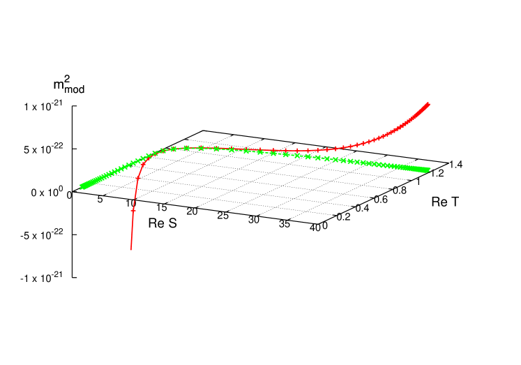
Figure 2: The lightest modulus mass squared on the $({\rm Re}\,S,{\rm Re}\,T)$-plane. The parameters are the same as in Fig. 1. The mass squared $m_{\rm mod}^{2}$ turns to be positive at $\alpha\simeq 7$.

Fig. 2 plots the lightest modulus mass squared $m_{\rm mod}^{2}$ and the SUSY point on the $({\rm Re}\,S,{\rm Re}\,T)$ plane. Again we vary $\alpha$ from 100 (left end-point) to 0.1 (right end-point) while fix the other parameters. Now we can see from this figure that the SUSY point near the M-theory limit (left end-point) is not local minimum since the lightest modulus is tachyonic, but this tachyonic mass squared monotonically increases as $\alpha$ decreases and becomes positive when $\left|c_{R}\right|\beta/\alpha\gg 1$. Thus the region around the SUSY RS limit ($\left|c_{R}\right|\beta/\alpha\gg 1$), where ${\rm Re}\,T>1$ is realized without any tachyonic masses, is the best candidate for the KKLT-type uplifting. We will study this region analytically in the following.

3.3.2 Analytic result near the RS limit

In the vicinity of $\alpha=0$, i.e., the SUSY RS model, the Kähler and the superpotentials in (3.1) are expressed as

$$K\!\!\! =\!\!\! -3\ln\left[\frac{1}{2\beta}\left\{1-\left|\Omega\right|^{2}+\frac{1-\left|\Omega\right|^{2}+\left|\Omega\right|^{2}\ln\left|\Omega\right|^{2}}{3q{\rm Re}\,S_{0}}+{\cal O}\left(\frac{1}{q^{2}({\rm Re}\,S_{0})^{2}}\right)\right\}\right]-\ln({\rm Re}\,S_{0}),$$

$$W\!\!\! =\!\!\! b_{0}\left\{(c+S_{0})(1-r\Omega^{3})+\frac{2r}{q}\Omega^{3}\ln\Omega\right\}.$$ (3.32)

Here $q\equiv\beta/\alpha$ times $\left|c_{R}\right|=\left|{\rm Re}\,c\right|$ is supposed to be large. Then from the SUSY conditions: $D_{S_{0}}W=D_{\Omega}W=0$, we find the SUSY point as

$$S_{0}\!\!\! =\!\!\! -c\left\{1-\frac{2}{3qc}\left(1-\frac{\ln r}{1-\rho^{-2/3}}\right)+{\cal O}\left((qc_{R})^{-2}\right)\right\},$$

$$\Omega\!\!\! =\!\!\! r^{-1/3}\left\{1-\frac{\ln r}{9qc_{R}}+{\cal O}\left((qc_{R})^{-2}\right)\right\}.$$ (3.33)

Here $r\equiv b_{\pi}/b_{0}$ and $\rho\equiv\left|r\right|$. Since the SUSY point in the pure $\beta$-gauging (3.25) is a local minimum of the potential, this point is also a local minimum when $q\left|c_{R}\right|\gg 1$. Due to the correction from the pure $\beta$-gauging case, the superpotential $W$ does not vanish at this point.

$$W=-\frac{2b_{0}\ln r}{3q}\left\{1+{\cal O}\left((qc_{R})^{-2}\right)\right\}.$$ (3.34)

Thus the vacuum energy becomes negative, evaluated as

$$V=-3e^{K}\left|W\right|^{2}=-\frac{32\beta^{3}\left|b_{0}\ln r\right|^{2}}{3q^{2}\left|c_{R}\right|(1-\rho^{-2/3})^{3}}\left\{1+{\cal O}\left(\frac{1}{qc_{R}}\right)\right\}.$$ (3.35)

Namely this is an AdS₄ SUSY vacuum.

3.4 Uplifting

So far we have found some stationary solutions of the scalar potential in the hybrid model assuming certain simple superpotential terms at the orbifold fixed points. In the heterotic M-theory limit (pure $\alpha$-gauging), the SUSY point is a saddle point. In the SUSY RS limit (pure $\beta$-gauging), on the other hand, the local minimum of the potential is a SUSY Minkowski vacuum.

Finding a SUSY breaking Minkowski minimum, which is a candidate of our present universe, is indeed a hard task in supergravity models. The hybrid model studied in this section is also the case. As mentioned in the introduction, the KKLT model provides an interesting and systematic way of achieving a SUSY breaking minimum with vanishing vacuum energy, that is, uplifting SUSY AdS minimum by a SUSY breaking vacuum energy which is assumed to be well sequestered from the light moduli as well as the visible sector. Here we consider the uplifting of the AdS SUSY minimum in our hybrid model by a SUSY breaking sector which is assumed to be well sequestered from $S_{0}$ and $\Omega$ (or $T$).

As mentioned at the end of Sec. 3.3.1, the region around the SUSY RS model ($q\left|c_{R}\right|\gg 1$) is the best candidate for the uplifting. So we consider such a parameter region which we discussed in Sec. 3.3.2. Following the KKLT model, the uplifting potential $U$ is assumed as [11, 36]

$$U\!\!\! =\!\!\! \int\!\!d^{4}\theta(\bar{\phi}\phi)^{n}\kappa\theta^{2}\bar{\theta}^{2}\ =\ \kappa e^{nK/3}$$ (3.36)

$$=\!\!\! \frac{\kappa(2\beta)^{n}}{({\rm Re}\,S_{0})^{n/3}(1-\left|\Omega\right|^{2})^{n}}\left\{1+{\cal O}\left(\frac{1}{qc_{R}}\right)\right\},$$

where $\kappa$ is a constant. The typical value of $n$ for the sequestered SUSY breaking source is given by $n=2$ [11, 36]. The total scalar potential is then given by $V_{\rm tot}\equiv V+U$. Then the local minimum $(S,\Omega)$ is shifted from the SUSY point (3.33) by

$$\delta S_{0}\!\!\! =\!\!\! \frac{2n\left|\ln r\right|^{2}}{27q^{2}(-c_{R})\rho^{4/3}(1-\rho^{-4/3})^{2}}\left\{1+{\cal O}\left(\frac{1}{qc_{R}}\right)\right\},$$

$$\delta\Omega\!\!\! =\!\!\! -\frac{2n\left|\ln r\right|^{2}}{54q^{2}(-c_{R})^{2}\rho^{5/3}(1-\rho^{-4/3})^{2}}\left\{1+{\cal O}\left(\frac{1}{qc_{R}}\right)\right\}.$$ (3.37)

Here we have chosen $\kappa$ as

$$\kappa=\frac{4(2\beta)^{3-n}\left|b_{0}\ln r\right|^{2}}{3q^{2}(-c_{R})^{1-n/3}(1-\rho^{-2/3})^{3-n}}\left\{1+{\cal O}\left(\frac{1}{qc_{R}}\right)\right\},$$ (3.38)

so that $V_{\rm tot}=0$ at the leading order in the $(qc_{R})^{-1}$-expansion.

Now we evaluate the F-terms of the chiral multiplets by the formulae,

$$F^{X}=-e^{K/2}K^{X\bar{Y}}D_{\bar{Y}}\bar{W},\;\;\;\;\;F^{\phi}=\frac{1}{3}e^{K/6}K_{X}F^{X}+e^{2K/3}\bar{W},$$ (3.39)

for $X,Y=S,\Omega$. These provides the SUSY breaking order parameters for the moduli mediation ($F^{X}$) and for the anomaly mediation ($F^{\phi}$). They are estimated at the uplifted Minkowski minimum as

$$F^{S}\!\!\! =\!\!\! {\cal O}(q^{-3}c_{R}^{-2}),$$

$$F^{\Omega}\!\!\! =\!\!\! -\frac{2ne^{-i\zeta/3}(2\beta)^{3/2}\bar{b}_{0}\left|\ln r\right|^{2}}{27q^{2}(-c_{R})^{3/2}\rho(1+\rho^{-2/3})^{2}(1-\rho^{-2/3})^{5/2}}\left\{1+{\cal O}\left(\frac{1}{qc_{R}}\right)\right\},$$

$$F^{\phi}\!\!\! =\!\!\! -\frac{2\bar{b}_{0}(2\beta)^{2}\ln\bar{r}}{3q(-c_{R})^{2/3}(1-\rho^{-2/3})^{2}}\left\{1+{\cal O}\left(\frac{1}{qc_{R}}\right)\right\}.$$ (3.40)

If we define the anomaly/modulus ratio of SUSY breaking as [11, 36]

$$\alpha_{A/M}\equiv\frac{1}{\ln(M_{\rm Pl}/m_{3/2})}\cdot\frac{F^{\phi}/\phi}{F^{T}/(T+\bar{T})},$$ (3.41)

we find in this case as

$$\alpha_{A/M}=\frac{qc_{R}}{\ln(M_{\rm Pl}/m_{3/2})}\left\{\frac{6\ln\rho}{n\ln r}\rho^{2/3}(1+\rho^{-2/3})^{2}(1-\rho^{-2/3})+{\cal O}\left(\frac{1}{qc_{R}}\right)\right\}.$$ (3.42)

Since $\rho\equiv\left|r\right|$ is related to $\rho=e^{3\pi\beta{\rm Re}\,T}$ from (3.25), we can see from (3.42) that $\left|\alpha_{A/M}\right|\gg 1$ unless $\beta$ is small. (Notice that ${\rm Re}\,T$ should be larger than the Planck length $M_{\rm Pl}^{-1}=1$.) Thus the anomaly mediation tends to be dominant in this model. However, for small values of $\beta$, the parameter $\rho$ is allowed to be of ${\cal O}(1)$ and the modulus mediated contribution can be comparable to that of the anomaly mediation. For example, $\left|\alpha_{A/M}\right|\simeq 1$ when $n=2$, $r=2$, $qc_{R}=-8$, $\ln(M_{\rm Pl}/m_{3/2})=4\pi^{2}$. In this case, the mirage mediation is realized. Finally note that the moduli masses, which are given by (3.31) at the leading of the $(qc_{R})^{-1}$-expansion, are much larger than the gravitino mass,

$$m_{3/2}^{2}=e^{K}\left|W\right|^{2}=\frac{32\beta^{3}\left|b_{0}\ln r\right|^{2}}{9q^{2}\left|c_{R}\right|(1-\rho^{-2/3})^{3}}\left\{1+{\cal O}\left(\frac{1}{qc_{R}}\right)\right\}.$$ (3.43)

4 Generalized Luty-Sundrum model ($\alpha=0$)

In the previous section we have studied the hybrid model in the case that $\gamma=0$, assuming simple boundary superpotentials. In this section we consider a case that $\alpha=0$ while $\beta$ and $\gamma$ are arbitrary, in which the hybrid model (2.14) and (2.15) is reduced to the SUSY RS model with an AdS curvature $k$ and an arbitrary bulk mass $m$ defined in Eq. (2.10) for the hypermultiplet. We now introduce generic perturbative superpotential terms (2.18) at the orbifold fixed points. The Kähler potential and the superpotential in this case are given by

$$K = -3\ln\int^{\pi{\rm Re}\,T}_{0}dt\,e^{-2kt}(1-e^{(3k-2m)t}|H|^{2})^{\frac{1}{3}},$$ (4.1)

$$W = \frac{1}{4}\sum_{\vartheta=0,\pi}e^{-3\vartheta kT}\sum_{n}w_{\vartheta}^{(n)}e^{n\vartheta\left(\frac{3}{2}k-m\right)T}H^{n}.$$ (4.2)

In the hypersurface $H=0$, this corresponds to the Luty-Sundrum model [18],

$$K\Big{|}_{H=0}\!\!\! =\!\!\! -3\ln\frac{1-e^{-k(T+\bar{T})}}{2k},\qquad W\Big{|}_{H=0}=\ \frac{1}{4}\left(w_{0}^{(0)}+w_{\pi}^{(0)}e^{-3kT}\right).$$ (4.3)

We would like to mention that if we take the limit $k\to 0$ in the Kähler potential while keeping a finite $k$ in the superpotential in (4.3), the model becomes equivalent to the KKLT model.

4.1 Supersymmetry condition

In the following we assume that $|w_{\vartheta}^{(2)}|$ is sufficiently large. Then $H$ would receive a heavy SUSY mass around $H=0$ and can be integrated out by $D_{H}W=0$, i.e., $H=0$, without affecting the low energy dynamics of $T$ [37]. Then the low energy effective theory is given by the Luty-Sundrum model (4.3).

The SUSY conditions: $D_{H}W=D_{T}W=0$ in the $H=0$ slice are given by

$$D_{H}W\Big{|}_{H=0} = \frac{1}{4}\left(w_{0}^{(1)}+e^{-\pi\left(\frac{3}{2}k+m\right)T}w_{\pi}^{(1)}\right)\ =\ 0,$$ (4.4)

$$D_{T}W\Big{|}_{H=0} = \frac{-3\pi k}{4(|e^{\pi kT}|^{2}-1)}\left(w_{0}^{(0)}+e^{-3\pi kT}|e^{\pi kT}|^{2}w_{\pi}^{(0)}\right)\ =\ 0.$$ (4.5)

In the following we further assume ${\rm Im}\,w_{\vartheta}^{(0)}={\rm Im}\,w_{\vartheta}^{(1)}=0$ ($\vartheta=0,\pi$) for simplicity. Then a solution for (4.4) and (4.5) is found as

$$T = \bar{T}\ =\ \ln\left(-\frac{w_{0}^{(1)}}{w_{\pi}^{(1)}}\right)^{-\frac{2}{\pi(3k+2m)}}\ =\ \ln\left(-\frac{w_{0}^{(0)}}{w_{\pi}^{(0)}}\right)^{-\frac{1}{\pi k}}.$$ (4.6)

In order for the above solution to be valid, the following relation must be satisfied.

$$-\frac{w_{0}^{(1)}}{w_{\pi}^{(1)}} = \left(-\frac{w_{0}^{(0)}}{w_{\pi}^{(0)}}\right)^{\frac{3k+2m}{2k}}.$$ (4.7)

One of the simplest choices satisfying (4.7) is

$$3k+2m = 0,\qquad w_{0}^{(1)}+w_{\pi}^{(1)}\ =\ 0.$$ (4.8)

Because the extension to the other cases is straightforward, we focus on the case (4.8) in the following. Then the SUSY point is summarized as

$$H = 0,\qquad T\ =\ T_{\rm SUSY}\ \equiv\ \ln\left(-\frac{w_{0}^{(0)}}{w_{\pi}^{(0)}}\right)^{-\frac{1}{\pi k}}$$ (4.9)

In our model we find from (3.5) that

$$V_{H\bar{H}} = e^{K}K_{H\bar{H}}^{-1}(|W_{HH}|^{2}-2K_{H\bar{H}}|W|^{2}),$$ (4.10)

$$V_{HH} = -e^{K}\bar{W}W_{HH},$$ (4.11)

$$V_{H\bar{T}} = V_{HT}\ =\ 0,$$ (4.12)

at the SUSY point (4.9). The mass-square eigenvalues of $({\rm Re}\,H,\,{\rm Im}\,H)$ are then given by

$$m_{H\pm}^{2} = K_{H\bar{H}}^{-1}(V_{H\bar{H}}\pm|V_{HH}|).$$ (4.13)

In order for the SUSY point (4.9) to be a local minimum, a condition $m^{2}_{H\pm}>0$ has to be satisfied, which results in

$$\left|\frac{W_{HH}}{W}\right| > \sqrt{\frac{1}{4}K_{H\bar{H}}^{2}+2K_{H\bar{H}}}+\frac{1}{2}K_{H\bar{H}},$$ (4.14)

where

$$\frac{W_{HH}}{W} = \frac{w_{\pi}^{(2)}+e^{-3\pi kT}w_{0}^{(2)}}{w_{0}^{(0)}+e^{-3\pi kT}w_{\pi}^{(0)}}\cdot 2e^{3\pi kT}$$ (4.15)

$$K_{H\bar{H}} = \frac{1-e^{-4\pi kT}}{1-e^{-2\pi kT}}\cdot\frac{1}{2}e^{4\pi kT},$$ (4.16)

and $e^{\pi kT}=-w_{\pi}^{(0)}/w_{0}^{(0)}$.

In the case $e^{\pi kT}\gg 1$, the condition (4.14) becomes

$$\left|\frac{w_{\pi}^{(2)}}{w_{0}^{(0)}}\right| > \frac{1}{4}e^{\pi kT}\ =\ \frac{1}{4}\cdot\frac{-w_{\pi}^{(0)}}{w_{0}^{(0)}},$$ (4.17)

which can be satisfied by, e.g.,

$$|w_{\pi}^{(2)}| > \frac{1}{4}|w_{\pi}^{(0)}|,\qquad w_{\pi}^{(0)}\ <\ 0,\qquad w_{0}^{(0)}\ >\ 0.$$ (4.18)

4.2 Moduli stabilization and uplifting

From (4.6), the SUSY point is given by

$$e^{-\pi kT} = w_{0}/w_{\pi}.$$ (4.19)

Here we choose the parameters as

$$w_{0}\equiv w_{0}^{(0)}\ >\ 0,\qquad w_{\pi}\equiv-w_{\pi}^{(0)}\ >\ 0,\qquad w_{0}/w_{\pi}\ \ll 1.$$ (4.20)

This SUSY point has a negative vacuum energy $V=-3m_{3/2}^{2}$ where

$$m_{3/2}^{2} = e^{K}|W|^{2}\ =\ \frac{k^{3}}{2}w_{0}^{2}(1-w_{0}^{2}/w_{\pi}^{2})^{2},$$ (4.21)

is the gravitino mass squared. The mass-square eigenvalues $m_{T\pm}^{2}$ of modulus $T$ at this point are given by

$$\left(m_{T+}^{2},m_{T-}^{2}\right) = \left(4m_{3/2}^{2},\ 0\right).$$ (4.22)

It is interesting that the stabilized value (4.19) of the modulus $T$ is the same as that of the KKLT model [11] in spite of the difference between their effective Kähler potentials. Note also that the former is the exact result while the latter is only an approximate one that is only valid for large $\pi kR$. Furthermore remark that the magnitudes of the mass eigenvalues (4.22) are smaller than those in the KKLT model $m_{T\pm}^{\rm KKLT}\simeq 2\pi kRm_{3/2}$ for $\pi kR\gg 1$. This is because the SUSY mass contributions from the Kähler potential is comparable to those from the superpotential in our model, and they partially ($m_{T+}^{2}$) or completely ($m_{T-}^{2}$) cancel each other.

Now we study the effect of the uplifting in this model. We uplift the AdS minimum (4.9) by a sequestered vacuum energy $U$ localized at $y=0$, given by

$$U = \int d\theta^{4}(\phi\bar{\phi})^{n}\kappa\theta^{2}\bar{\theta}^{2}\ =\ \kappa e^{nK/3}.$$ (4.23)

The total scalar potential is thus $V_{\rm tot}\equiv V+U$, and the minimum would be shifted as $T=T_{\rm SUSY}+\delta T$. We tune the constant $\kappa$ as

$$\kappa = 3e^{-nK/3}m_{3/2}^{2}\ =\ 3\left(\frac{1-w_{0}^{2}/w_{\pi}^{2}}{2k}\right)^{n}m_{3/2}^{2},$$ (4.24)

so that $V+U=0$ at the leading order in the $\delta T/T_{\rm SUSY}$ expansion. Then we find the shift of $T$ at this Minkowski minimum as

$$\delta T = \frac{n}{2k(2+n)},$$ (4.25)

which can be small for $k\gg 1$ and $n={\cal O}(1)$. The SUSY breaking order parameter at this minimum is found as

$$F^{T} = \frac{n}{2k}\cdot\frac{w_{\pi}^{2}-w_{0}^{2}}{(2+n)w_{\pi}^{2}+n^{2}w_{0}^{2}}\,m_{3/2}^{2}.$$ (4.26)

The anomaly/modulus ratio of SUSY breaking $\alpha_{A/M}$ defined in Eq. (3.41) is calculated in this case as

$$\alpha_{A/M} \simeq 4(1+2/n).$$ (4.27)

Then $\alpha_{A/M}=8$ for the typical value $n=2$ in the uplifting potential, and the anomaly mediation seems to be dominant. This should be compared with $\alpha_{A/M}=1$ in the KKLT model which corresponds to an asymmetric limit of our model, that is, $k\to 0$ in the Kähler potential keeping $k$ finite in the superpotential in (4.3).

5 Summary

We studied the 4D effective theory of the 5D gauged supergravity on an orbifold with a universal hypermultiplet and superpotential terms at the orbifold fixed points. We analyzed a class of models obtained by gauging three independent isometries on the scalar manifold. It includes, as different limits, both the 5D heterotic M-theory and the SUSY RS model with an arbitrary bulk mass parameter for the hypermultiplet. We have investigated the vacuum structure of such models and the nature of moduli stabilization assuming perturbative superpotential terms at the fixed points, and discussed the uplifting of SUSY AdS vacua.

First we analyzed the hybrid model in a case that the Kähler and the superpotentials in the effective action have analytic expressions, i.e., $(\alpha,\beta)$-gauging. In the heterotic M-theory limit (pure $\alpha$-gauging), the SUSY point is a saddle point of the potential, and the local minimum is not supersymmetric. The potential energies at these points are both negative, and thus the 4D geometry is AdS₄. In the SUSY RS limit (pure $\beta$-gauging), on the other hand, the SUSY point is a local minimum with vanishing vacuum energy when the parameters satisfy the relation (3.22) with $c_{R}<0$. Namely this is a SUSY Minkowski vacuum. We have shown numerically that both SUSY points continuously transit to each other by changing the ratio $q=\beta/\alpha$, and find that the region around the SUSY RS limit ($q\left|c_{R}\right|\gg 1$) is the best candidate for the KKLT-type uplifting. Thus we analytically studied the uplifting of the SUSY AdS₄ vacuum in the vicinity of the SUSY RS limit. For small values of $\beta$, the mirage mediation ($\alpha_{A/M}={\cal O}(1)$) can be realized while the effect of the anomaly mediation is dominant for $\beta\stackrel{{\scriptstyle>}}{{{}_{\sim}}}{\cal O}(1)$. The moduli are much heavier than the gravitino in both cases.

We also analyzed the SUSY RS model with an arbitrary bulk mass parameter, i.e., $(\beta,\gamma)$-gauging, and generic perturbative superpotential terms at the fixed points. If the mass parameter $w_{\vartheta}^{(2)}$ in the boundary superpotential is large enough, the matter field $H$ is stabilized at $H=0$ prior to the radion $T$, and the model is reduced to the Luty-Sundrum model [18] in the $H=0$ slice. Note that taking a limit $k\to 0$ in the Kähler potential while keeping finite $k$ in the superpotential in (4.3) gives an equivalent effective theory to the KKLT model. In contrast to the KKLT model, the exponential terms for the modulus $T$ does not originate from any nonperturbative effects but from the warped geometry generated by the $\beta$-gauging. We find a SUSY AdS vacuum in this model which can be uplifted to a Minkowski vacuum by a sequestered SUSY breaking vacuum energy just like the KKLT model, yielding a certain anomaly/modulus ratio of the SUSY breaking mediation, $\alpha_{A/M}\simeq 8$. Note that the KKLT-type uplifting sector adopted in this paper can be easily extended to some dynamical SUSY breaking models like O’Raifeartaigh model [38] or Intriligator-Seiberg-Shih model [39] as has been done in Ref. [13].

In this paper we have considered only a case that the boundary superpotentials are polynomials for the hypermultiplet and there are no $Z_{2}$-odd vector multiplets other than the graviphoton multiplet. It would be important to include nonperturbative effects for the study of moduli stabilization in more general setup. For the 5D heterotic M-theory, this kind of study has been done extensively in Refs. [24, 40]. The nonperturbative effects such as the gaugino condensations generically depend on the gauge couplings, and thus depend on the moduli which determine the latter. The moduli dependence of the gauge couplings in the effective theory of 5D supergravity is determined by the coefficients $C_{IJK}$ in the cubic polynomial ${\cal N}$ in Eq.(2.3), (which is referred to as the Calabi-Yau intersection numbers in the 5D heterotic M-theory). Depending on those coefficients, we could have moduli mixings in the gauge couplings which play important role [37, 41, 42] in the moduli stabilization with the nonperturbative effects. We will study these cases in our future works.

Acknowledgements

H. A. and Y. S. are supported by the Japan Society for the Promotion of Science for Young Scientists (No.182496 and No.179241, respectively).

Appendix A Isometries in on-shell description

Here we see how $SU(2,1)$ isometries are realized in the on-shell description of 5D supergravity. In order to move to the on-shell Poincaré supergravity, we have to fix the extraneous superconformal symmetries by imposing the gauge-fixing conditions [19]-[22]. The explicit forms of these gauge-fixing conditions in our notation are listed in the appendix A of Ref. [25]. Since we have two compensator hypermultiplets, we also have to use the gauge-fixing for $U(1)_{T}$ and the equations of motion for the auxiliary fields in the $U(1)_{T}$ vector multiplet to eliminate the whole degrees of freedom for the compensator scalars. Using all the above conditions, the hyperscalars $\varphi^{a}$ ($a=1,2,\ldots,6$) are expressed in terms of the physical scalar fields $(S,\xi)$, which are identified with those appearing in Ref. [28], as

$$\varphi^{1}\!\!\! =\!\!\! 0,\;\;\;\;\;\varphi^{2}=\left\{\frac{S+\bar{S}}{2(S+\bar{S}-2\left|\xi\right|^{2})}\right\}^{1/2},$$

$$\varphi^{3}\!\!\! =\!\!\! \frac{\left|1+S\right|}{2(S+\bar{S})^{1/2}},\;\;\;\;\;\varphi^{4}=\varphi^{2}\frac{\bar{\xi}(1-S)}{S+\bar{S}},$$

$$\varphi^{5}\!\!\! =\!\!\! \varphi^{3}\frac{1-S}{1+S},\;\;\;\;\;\varphi^{6}=\varphi^{2}\frac{\bar{\xi}(1+S)}{S+\bar{S}}.$$ (A.1)

Under the orbifold parity, $S$ and $\xi$ are even and odd, respectively. From (A.1) we can also express $S$ and $\xi$ by $\varphi^{a}$ ($a=1,2,\ldots,6$) as

$$S=\frac{\varphi^{3}-\varphi^{5}}{\varphi^{3}+\varphi^{5}},\;\;\;\;\;\xi=\frac{\varphi^{3}\bar{\varphi}^{6}-\varphi^{5}\bar{\varphi}^{4}}{\bar{\varphi}^{2}(\varphi^{3}+\varphi^{5})}.$$ (A.2)

Note that Eq.(A.2) holds only in a gauge where $\varphi^{1}=0$.

Now we consider the $SU(2,1)$ transformations of $\varphi^{a}$. They are given by

$$\begin{pmatrix}\varphi^{\prime 1}\\ \varphi^{\prime 3}\\ \varphi^{\prime 5}\end{pmatrix}=e^{i\tilde{\alpha}\cdot T}\begin{pmatrix}\varphi^{1}\\ \varphi^{3}\\ \varphi^{5}\end{pmatrix},\;\;\;\;\;\begin{pmatrix}\varphi^{\prime 2}\\ \varphi^{\prime 4}\\ \varphi^{\prime 6}\end{pmatrix}=\left(e^{i\tilde{\alpha}\cdot T}\right)^{*}\begin{pmatrix}\varphi^{2}\\ \varphi^{4}\\ \varphi^{6}\end{pmatrix},$$ (A.3)

where $\tilde{\alpha}\cdot T\equiv\sum_{i=1}^{8}\tilde{\alpha}_{i}T^{i}$ and $\tilde{\alpha}_{i}$ are the real transformation parameters. The $SU(2,1)$ generators $T^{i}$ ($i=1,2,\ldots,8$) are given by

$$T^{1} = \begin{pmatrix}0&1&0\\ 1&0&0\\ 0&0&0\end{pmatrix},\ T^{2}\ =\ \begin{pmatrix}0&-i&0\\ i&0&0\\ 0&0&0\end{pmatrix},\ T^{3}\ =\ \begin{pmatrix}1&0&0\\ 0&-1&0\\ 0&0&0\end{pmatrix},$$

$$T^{4} = \begin{pmatrix}0&0&1\\ 0&0&0\\ -1&0&0\end{pmatrix},\ T^{5}\ =\ \begin{pmatrix}0&0&i\\ 0&0&0\\ i&0&0\end{pmatrix},\ T^{6}\ =\ \begin{pmatrix}0&0&0\\ 0&0&1\\ 0&-1&0\end{pmatrix},$$

$$T^{7} = \begin{pmatrix}0&0&0\\ 0&0&i\\ 0&i&0\end{pmatrix},\ T^{8}\ =\ \begin{pmatrix}0&0&0\\ 0&1&0\\ 0&0&-1\end{pmatrix}.$$ (A.4)

After the transformation (A.3), the compensator scalar $\varphi^{\prime 1}$ are in general nonzero. We can move to a gauge where $\varphi^{\prime\prime 1}=0$ by using $SU(2)_{\mbox{\scriptsize${\mbox{\boldmath$U$}}$}}$, which is part of the superconformal symmetries the off-shell 5D supergravity has. Then the other scalar components become

$$\varphi^{\prime\prime 2\hat{a}-1}\!\!\! =\!\!\! \frac{\cos\theta_{\mbox{\scriptsize${\mbox{\boldmath$U$}}$}}}{\left|\varphi^{\prime 2}\right|}\left(\bar{\varphi}^{\prime 2}\varphi^{\prime 2\hat{a}-1}-\varphi^{\prime 1}\bar{\varphi}^{\prime 2\hat{a}}\right),\;\;\;\;\;(\hat{a}=2,3)$$

$$\varphi^{\prime\prime 2\hat{a}}\!\!\! =\!\!\! \frac{\cos\theta_{\mbox{\scriptsize${\mbox{\boldmath$U$}}$}}}{\left|\varphi^{\prime 2}\right|}\left(\varphi^{\prime 1}\bar{\varphi}^{\prime 2\hat{a}-1}+\bar{\varphi}^{\prime 2}\varphi^{\prime 2\hat{a}}\right),\;\;\;\;\;(\hat{a}=1,2,3)$$ (A.5)

where $\theta_{\mbox{\scriptsize${\mbox{\boldmath$U$}}$}}\equiv\arctan\left|\varphi^{\prime 1}/\bar{\varphi}^{\prime 2}\right|$. Since $\varphi^{\prime\prime 1}=0$, we can use (A.2) and express the transformed physical scalars $(S^{\prime\prime},\xi^{\prime\prime})$ in terms of the untransformed scalars $\varphi^{a}$, which are rewritten in terms of $(S,\xi)$ by the relation (A.1). Then we obtain the $SU(2,1)$ transformations of $(S,\xi)$. For example,

$$(S,\xi) \to \left(S-2i\tilde{\alpha}\xi+\tilde{\alpha}^{2},\xi+i\tilde{\alpha}\right)\;\;\;\;\;\mbox{for $\tilde{\alpha}\cdot T=-\tilde{\alpha}(T^{1}+T^{4})$}$$ (A.6)

$$\to \left(S+2i\tilde{\alpha},\xi\right),\;\;\;\;\;\mbox{for $\tilde{\alpha}\cdot T=\tilde{\alpha}(T^{6}+T^{8})$}$$

$$\to (e^{2\tilde{\alpha}}S,e^{\tilde{\alpha}}\xi),\;\;\;\;\;\mbox{for $\tilde{\alpha}\cdot T=\tilde{\alpha}T^{7}$}$$

$$\to (S,e^{-3i\tilde{\alpha}}\xi).\;\;\;\;\;\mbox{for $\tilde{\alpha}\cdot T=\tilde{\alpha}(2T^{3}+T^{8})$}$$

These transformations correspond to those of Eqs.(16),(18),(19) and (20) in the published version of Ref. [28]. However we can show that there is no choice of $\tilde{\alpha}_{i}$ that realizes the transformation (17) in Ref. [28], which we believe is their typographical error. On the other hand, it is easy to check that the isometries generated by the Killing vectors in (3.12) of Ref. [27] are identical to those derived in the above way. For small $\tilde{\alpha}_{i}$ ($i=1,2,\ldots,8$), general $SU(2,1)$ transformations of $S$ and $\xi$ are given by

$$S \to S+i\left\{\left(-\frac{\tilde{\alpha}_{3}}{2}+\tilde{\alpha}_{6}+\tilde{\alpha}_{8}\right)-2i\tilde{\alpha}_{7}S+\left(\bar{\alpha}_{12}+\alpha_{45}\right)\xi\right.$$

$$\hskip 42.67912pt\left.+\left(\bar{\alpha}_{12}-\alpha_{45}\right)S\xi+\left(\frac{\tilde{\alpha}_{3}}{2}+\tilde{\alpha}_{6}-\tilde{\alpha}_{8}\right)S^{2}\right\}+{\cal O}(\tilde{\alpha}^{2}),$$

$$\xi \to \xi+i\left\{-\frac{\alpha_{12}+\bar{\alpha}_{45}}{2}+\frac{\alpha_{12}-\bar{\alpha}_{45}}{2}S-\left(\frac{3}{2}\tilde{\alpha}_{3}+i\tilde{\alpha}_{7}\right)\xi\right.$$ (A.7)

$$\hskip 42.67912pt\left.+\left(\frac{\tilde{\alpha}_{3}}{2}+\tilde{\alpha}_{6}-\tilde{\alpha}_{8}\right)S\xi+\left(\bar{\alpha}_{12}-\alpha_{45}\right)\xi^{2}\right\}+{\cal O}(\tilde{\alpha}^{2}),$$

where $\alpha_{12}\equiv\tilde{\alpha}_{1}+i\tilde{\alpha}_{2}$ and $\alpha_{45}\equiv\tilde{\alpha}_{4}+i\tilde{\alpha}_{5}$.

References

• [1] L. Randall and R. Sundrum, Phys. Rev. Lett.  83, 3370 (1999) [arXiv:hep-ph/9905221].
• [2] R. Altendorfer, J. Bagger and D. Nemeschansky, Phys. Rev.  D 63, 125025 (2001) [arXiv:hep-th/0003117]; A. Falkowski, Z. Lalak and S. Pokorski, Phys. Lett.  B 491, 172 (2000) [arXiv:hep-th/0004093].
• [3] T. Gherghetta and A. Pomarol, Nucl. Phys.  B 586, 141 (2000) [arXiv:hep-ph/0003129].
• [4] N. Arkani-Hamed and M. Schmaltz, Phys. Rev.  D 61, 033005 (2000) [arXiv:hep-ph/9903417].
• [5] L. Randall and R. Sundrum, Nucl. Phys.  B 557, 79 (1999) [arXiv:hep-th/9810155]; G. F. Giudice, M. A. Luty, H. Murayama and R. Rattazzi, JHEP 9812, 027 (1998) [arXiv:hep-ph/9810442].
• [6] J. M. Maldacena, Adv. Theor. Math. Phys.  2, 231 (1998) [Int. J. Theor. Phys.  38, 1113 (1999)] [arXiv:hep-th/9711200]; N. Arkani-Hamed, M. Porrati and L. Randall, JHEP 0108, 017 (2001) [arXiv:hep-th/0012148].
• [7] P. Horava and E. Witten, Nucl. Phys.  B 460, 506 (1996) [arXiv:hep-th/9510209]; P. Horava and E. Witten, Nucl. Phys.  B 475, 94 (1996) [arXiv:hep-th/9603142].
• [8] A. Lukas, B. A. Ovrut, K. S. Stelle and D. Waldram, Phys. Rev.  D 59, 086001 (1999) [arXiv:hep-th/9803235]; A. Lukas, B. A. Ovrut, K. S. Stelle and D. Waldram, Nucl. Phys.  B 552, 246 (1999) [arXiv:hep-th/9806051].
• [9] S. Kachru, R. Kallosh, A. Linde and S. P. Trivedi, Phys. Rev.  D 68, 046005 (2003) [arXiv:hep-th/0301240].
• [10] S. B. Giddings, S. Kachru and J. Polchinski, Phys. Rev.  D 66, 106006 (2002) [arXiv:hep-th/0105097].
• [11] K. Choi, A. Falkowski, H. P. Nilles, M. Olechowski and S. Pokorski, JHEP 0411, 076 (2004) [arXiv:hep-th/0411066];
• [12] A. Saltman and E. Silverstein, JHEP 0411, 066 (2004) [arXiv:hep-th/0402135]; M. Gomez-Reino and C. A. Scrucca, JHEP 0605, 015 (2006) [arXiv:hep-th/0602246]; O. Lebedev, H. P. Nilles and M. Ratz, Phys. Lett.  B 636, 126 (2006) [arXiv:hep-th/0603047]; Z. Lalak, O. J. Eyton-Williams and R. Matyszkiewicz, JHEP 0705, 085 (2007) [arXiv:hep-th/0702026];
• [13] E. Dudas, C. Papineau and S. Pokorski, JHEP 0702, 028 (2007) [arXiv:hep-th/0610297]; H. Abe, T. Higaki, T. Kobayashi and Y. Omura, Phys. Rev.  D 75, 025019 (2007) [arXiv:hep-th/0611024]; R. Kallosh and A. Linde, JHEP 0702, 002 (2007) [arXiv:hep-th/0611183]; O. Lebedev, V. Lowen, Y. Mambrini, H. P. Nilles and M. Ratz, JHEP 0702, 063 (2007) [arXiv:hep-ph/0612035]; H. Abe, T. Higaki and T. Kobayashi, arXiv:0707.2671 [hep-th].
• [14] C. P. Burgess, R. Kallosh and F. Quevedo, JHEP 0310, 056 (2003) [arXiv:hep-th/0309187]; A. Achucarro, B. de Carlos, J. A. Casas and L. Doplicher, JHEP 0606, 014 (2006) [arXiv:hep-th/0601190]; S. L. Parameswaran and A. Westphal, JHEP 0610, 079 (2006) [arXiv:hep-th/0602253]; K. Choi and K. S. Jeong, JHEP 0608, 007 (2006) [arXiv:hep-th/0605108]; S. L. Parameswaran and A. Westphal, Fortsch. Phys.  55, 804 (2007) [arXiv:hep-th/0701215].
• [15] J. M. Maldacena and C. Nunez, Int. J. Mod. Phys.  A 16, 822 (2001) [arXiv:hep-th/0007018]; B. de Wit, D. J. Smit and N. D. Hari Dass, Nucl. Phys.  B 283, 165 (1987).
• [16] K. Choi, K. S. Jeong and K. i. Okumura, JHEP 0509, 039 (2005) [arXiv:hep-ph/0504037].
• [17] M. Endo, M. Yamaguchi and K. Yoshioka, Phys. Rev.  D 72, 015004 (2005) [arXiv:hep-ph/0504036].
• [18] M. A. Luty and R. Sundrum, Phys. Rev.  D 64, 065012 (2001) [arXiv:hep-th/0012158].
• [19] T. Kugo and K. Ohashi, Prog. Theor. Phys.  105, 323 (2001) [arXiv:hep-ph/0010288];
• [20] T. Fujita and K. Ohashi, Prog. Theor. Phys.  106, 221 (2001) [arXiv:hep-th/0104130];
• [21] T. Fujita, T. Kugo and K. Ohashi, Prog. Theor. Phys.  106, 671 (2001) [arXiv:hep-th/0106051].
• [22] T. Kugo and K. Ohashi, Prog. Theor. Phys.  108, 203 (2002) [arXiv:hep-th/0203276].
• [23] F. Paccetti Correia, M. G. Schmidt and Z. Tavartkiladze, Nucl. Phys.  B 709, 141 (2005) [arXiv:hep-th/0408138]; H. Abe and Y. Sakamura, JHEP 0410, 013 (2004) [arXiv:hep-th/0408224].
• [24] F. P. Correia, M. G. Schmidt and Z. Tavartkiladze, Nucl. Phys.  B 751, 222 (2006) [arXiv:hep-th/0602173].
• [25] H. Abe and Y. Sakamura, Phys. Rev.  D 75, 025018 (2007) [arXiv:hep-th/0610234].
• [26] M. Kaku, P.K. Townsend and P. Van Nieuwenhuizen, Phys. Rev. Lett. 39, 1109 (1977); Phys. Lett. B 69, 304 (1977); Phys. Rev. D 17, 3179 (1978); T. Kugo and S. Uehara, Nucl. Phys. B 226, 49 (1983); Prog. Theor. Phys. 73, 235 (1985).
• [27] A. Ceresole, G. Dall’Agata, R. Kallosh and A. Van Proeyen, Phys. Rev. D 64, 104006 (2001) [arXiv:hep-th/0104056].
• [28] A. Falkowski, Z. Lalak and S. Pokorski, Phys. Lett.  B 509, 337 (2001) [arXiv:hep-th/0009167].
• [29] E. Bergshoeff, R. Kallosh and A. Van Proeyen, JHEP 0010, 033 (2000) [arXiv:hep-th/0007044].
• [30] H. Abe and Y. Sakamura, Phys. Rev.  D 71, 105010 (2005) [arXiv:hep-th/0501183]; H. Abe and Y. Sakamura, Phys. Rev.  D 73, 125013 (2006) [arXiv:hep-th/0511208].
• [31] A. Lukas, B. A. Ovrut and D. Waldram, Nucl. Phys.  B 532, 43 (1998) [arXiv:hep-th/9710208].
• [32] P. Breitenlohner and D.Z. Freedman, Phys. Lett. 115B, 197 (1982).
• [33] B. de Carlos, S. Gurrieri, A. Lukas and A. Micu, JHEP 0603, 005 (2006) [arXiv:hep-th/0507173].
• [34] N. Maru and N. Okada, Phys. Rev.  D 70, 025002 (2004) [arXiv:hep-th/0312148].
• [35] N. Maru, N. Sakai and N. Uekusa, Phys. Rev.  D 75, 125014 (2007) [arXiv:hep-th/0612071]; N. Maru, N. Sakai and N. Uekusa, Phys. Rev.  D 74, 045017 (2006) [arXiv:hep-th/0602123].
• [36] K. Choi, arXiv:0705.3330 [hep-th].
• [37] H. Abe, T. Higaki and T. Kobayashi, Phys. Rev.  D 74, 045012 (2006) [arXiv:hep-th/0606095].
• [38] L. O’Raifeartaigh, Nucl. Phys.  B 96, 331 (1975).
• [39] K. Intriligator, N. Seiberg and D. Shih, JHEP 0604, 021 (2006) [arXiv:hep-th/0602239].
• [40] F. P. Correia, M. G. Schmidt and Z. Tavartkiladze, Nucl. Phys.  B 763, 247 (2007) [arXiv:hep-th/0608058]; F. P. Correia and M. G. Schmidt, arXiv:0708.3805 [hep-th].
• [41] H. Abe, T. Higaki and T. Kobayashi, Nucl. Phys.  B 742, 187 (2006) [arXiv:hep-th/0512232].
• [42] H. Abe, T. Higaki and T. Kobayashi, Phys. Rev.  D 73, 046005 (2006) [arXiv:hep-th/0511160].