Two-proton radioactivity

Abstract

In the first part of this review, experimental results which lead to the discovery of two-proton radioactivity are examined. Beyond two-proton emission from nuclear ground states, we also discuss experimental studies of two-proton emission from excited states populated either by nuclear $\beta$ decay or by inelastic reactions. In the second part, we review the modern theory of two-proton radioactivity. An outlook to future experimental studies and theoretical developments will conclude this review.

Version:

1 Introduction

Atomic nuclei are made of two distinct particles, the protons and the neutrons. These nucleons constitute more than 99.95% of the mass of an atom. In order to form a stable atomic nucleus, a subtle equilibrium between the number of protons and neutrons has to be respected. This condition is fulfilled for 259 different combinations of protons and neutrons. These nuclei can be found on Earth. In addition, 26 nuclei form a quasi stable configuration, i.e. they decay with a half-life comparable or longer than the age of the Earth and are therefore still present on Earth.

These stable or quasi-stable nuclei are characterised by an approximately equal number of neutrons and protons for light nuclei, whereas going to heavier nuclei the neutron excess increases to reach N-Z=44 for the heaviest stable nucleus ²⁰⁸Pb. In addition to these 285 stable or quasi-stable nuclei, some 4000-6000 unstable nuclei are predicted to exist, the exact number depending on the theoretical model used. Close to 2500 nuclei have been observed already. These unstable radioactive nuclei can be classified into seven categories depending on their decay modes: i) $\alpha$ emitters (about 375) which decay by ejecting a ⁴He nucleus, ii) $\beta^{+}$ emitters (1040) which transform a proton into a neutron plus a positron and a neutrino, or by capturing an electron from their atomic shells and emitting a neutrino, iii) $\beta^{-}$ emitters (1020) which transform a neutron into a proton by emitting an electron and an anti-neutrino, iv) fissioning nuclei (30) which split up into two roughly equal pieces, v) one-proton (1p) emitters (about 25), vi) two-proton (2p) emitters (2) and, finally, (vii) exotic-cluster emitters (about 25 different nuclei emitting fragments of C, O, F, Ne, Mg, and Si). These exotic radioactivities with masses from 14 to 32 may be considered as intermediate between $\alpha$ decay and fission. However, it should be mentioned that this decay mode is never dominant.

Although some radioactive nuclei can decay by two or three of these different decay modes, the main decay mode is dictated by the proton-to-neutron ratio. For example, nuclei with a modest proton excess decay by $\beta^{+}$ disintegration. If the proton excess increases, the nuclear forces can no longer bind all protons and one reaches the proton drip line where the spontaneous emission of protons takes place from the ground state. Heavier neutron-deficient isotopes will preferentially decay by $\alpha$ emission, and for the heaviest nuclei fission is the dominant decay mode. For some of the heaviest nuclei, exotic-cluster emission is a small decay branch.

The study of these different decay types started with the discovery of radioactivity by H. Becquerel in 1896. Following the work of Pierre and Marie Curie, E. Rutherford in 1899 classified the observed radioactivity into two different decay modes ($\alpha$ and $\beta$ rays) according to the detected particle in the decay. P. Villard discovered $\gamma$ radiation in 1900 as a third radioactive decay mode. Finally, the nuclear fission process was observed for the first time by O. Hahn and F. Strassmann and correctly explained by L. Meitner in 1938.

These ”classical” decay modes have helped largely to understand the structure of the atomic nucleus and the forces acting in the nucleus. They have also found many applications which range from solid-state physics to astrophysics and medicine. With the discovery of a large number of new radioactive isotopes the understanding of nuclear structure advanced as well.

Beginning of the 1960’s, Goldanskii [1], Zel’dovich [2], and Karnaukhov [3] proposed new types of proton radioactivity in very proton-rich nuclei. For nuclei with an odd number of protons, one-proton radioactivity was predicted. This decay mode was indeed observed at the beginning of the 1980’s in experiments at GSI, Darmstadt [4, 5]. Today about 25 ground-state one-proton emitters are known [6]. Proton emission was also observed in many cases from long-lived excited states, the first being ^53mCo [7, 8, 9]. The study of one-proton radioactivity allowed testing the nuclear mass surface, to determine the sequence of single-particle levels and the detailed structure of the wave function of the emitted proton (”$j$ content” of the wave function), and to investigate nuclear deformation beyond the proton drip line.

Zel’dovich [2] was probably the first to mention the possibility that nuclei may emit a pair of protons. However, it was Goldanskii [1, 10, 11, 12, 13] and Jänecke [14] who first tried to determine candidates for 2p radioactivity. Many others followed and the latest predictions [15, 16, 17] determined that ³⁹Ti, ⁴²Cr, ⁴⁵Fe, and ^49,48Ni should be the best candidates to discover this new decay mode. Goldanskii [1] also coined the name ”two-proton radioactivity” and it was Galitsky and Cheltsov [18] who proposed a first theoretical attempt to describe the process of 2p emission. More than 40 years after its theoretical proposal, 2p radioactivity was discovered [19, 20] in the decay of ⁴⁵Fe. In later experiments, ⁵⁴Zn [21] and most likely ⁴⁸Ni [22] were also shown to decay by two-proton radioactivity. The observation of two-proton emission from a long-lived nuclear ground state was preceded by the observation of two-proton emission from very short-lived nuclear ground state, e.g. in the cases of ⁶Be [23] and ¹²O [24], and by the emission of two protons from excited states populated by $\beta$ decay [25] or inelastic reactions [26]. A particular case is the emission of two protons from an isomer in ⁹⁴Ag^m [27].

The 2p emission process leads from an initial unbound state to a final state of separated fragments interacting by the Coulomb force. This transition to the final state can be realized in many ways, such as the sequential two-body decay via an intermediate resonance, the virtual sequential two-body decay via the correlated continuum of an intermediate nucleus, the direct decay into the three-particle continuum or its particular diproton (’²He’) limit of two sequential two-body emissions.

Different types of theoretical approaches exist which focus on the three-body decay width: the extended R-matrix theory [28, 29], the real-energy continuum shell model (the so-called Shell Model Embedded in the Continuum (SMEC)  [30, 31, 32, 33, 34]) describing sequential two-body emission, virtual sequential two-body emission and diproton emission via two sequential two-body emissions [33, 34], the Gamow Shell Model (GSM) with no separation between two- and three-body decays from the multi-particle continuum [35], the three-body models with outgoing flux describing direct decay into the continuum [36], the three-body models combined with complex coordinate scaling [37], or the Faddeev equations combined with either outgoing flux or complex scaling [38].

In the 2p decay, the three-body decay width provides global information with weighted contributions of different decay paths leading from the initial to the final state. Hence, the value of the width by itself does not reveal the dominant transition mechanism. In the theoretical analysis however, one can switch off certain decay paths and look for the three-body partial decay width resulting from a particular decay path. This strategy is used in the SMEC analysis of the experimental results. Obviously, the conclusions of such partial studies of decay mechanisms are not unambiguous.

In the present review, we will summarize the state of the art of experimental and theoretical studies on two-proton radioactivity. Previous reviews, written before the actual discovery of ground-state two-proton radioactivity, can be found in [39, 40].

2 Basic concepts for one- and two-proton radioactivity

Protons are charged particles, therefore they are sensitive to the charge of other protons which create a Coulomb barrier. This barrier prevents protons from quickly leaving the atomic nucleus even if they are unbound. The tunnelling probability depends on the available energy and the height of the Coulomb barrier, which in turn depends on the nuclear charge Z (number of protons) (see Fig. 1). The barrier penetration can give rise to measurable half-lives, if a certain balance between the available decay energy and the barrier height is respected. Fig. 2 shows in a simple model the relation between barrier penetration half-life and decay energy for different nuclear charges Z. In general, the higher is the available energy, the shorter is the tunnelling time. In turn, for higher Z more energy is needed for the same tunnelling time.

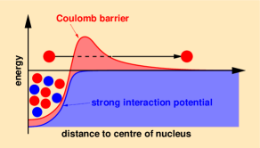
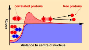
Figure 1: Due to their charge the protons have to tunnel through the Coulomb barrier generated by other protons. For one-proton emission (left), the tunnelling depends mainly on the barrier height. For two-proton emission (right) the correlation between the two protons most likely influences the tunnelling process. Figure courtesy of J. Giovinazzo.

The delay associated with the tunnelling process allows for the observation of 1p and 2p radioactivity. Even if protons are unbound by e.g. 1 MeV, the tunnelling of the combined Coulomb and centrifugal barriers is not instantaneous, i.e. the nuclear decay is delayed by a measurable amount of time. However, due to experimental constraints, mainly linked to the techniques used to study 1p or 2p radioactivity and due to the competition with $\beta^{+}$ decay, observation limits exist. The lower half-life limit of about 1 $\mu$s comes from the fact that often the observation of the 1p or 2p emitter is accomplished with the same detection setup which is used to detect the decay of these nuclei. This means that a decay signal of typically 1 MeV has to be observed a very short time after an identification signal (i.e. an implantation signal in a silicon detector) of several hundred MeV. This observation limit has been reached in 1p-emitter studies (see Sect. 3). The upper limit (see Fig. 2) strongly depends on the structure of the decaying nucleus which governs the $\beta$-decay half-life. It can range from a few milliseconds to a few seconds. To observe charged-particle emission, the barrier-penetration half-life should be comparable or shorter than the $\beta$-decay half-life.

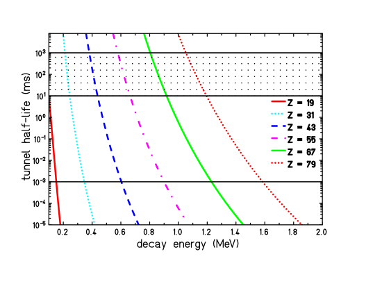
Figure 2: Barrier penetration half-lives for a proton as a function of the nuclear charge and the decay energy. The half-lives are calculated from Coulomb wave functions using the Wigner single-particle width (see e.g. [15]). The horizontal line gives the lower detection time limit, whereas the hatched area gives typical $\beta$-decay half-lives.

In the 1p decay, there are only two particles in the final state and the decay is a simple back-to-back decay, where the energy is shared between the two partners, the heavy recoil and the emitted proton, according to energy and momentum conservation.

In the case of 2p decay, the situation is more complicated (see Fig. 1). The decay characteristics depend sensitively on the decay pattern itself. Two schematical pictures are usually used to represent possible limiting cases: i) the three-body decay and ii) the diproton decay. In the former case, the two protons do not have any correlation beyond the phase-space constraints, which means that only energy and momentum conservation have to be respected. Such a decay pattern yields an isotropic angular distribution of protons which share the total decay energy, with individual proton energies ranging from zero to the total decay energy. A more realistic discussion of the tunnelling process changes this picture because the barrier penetration strongly favours an emission of two protons with similar energies. In the latter case of diproton emission, one assumes that a pre-formed ’²He’-cluster penetrates the Coulomb barrier and decays outside the barrier. The decay half-life depends sensibly on the ²He resonance energy. The diproton decay corresponds to two sequential binary decays for which the kinematics is rather easy.

These two limits of 2p decay are not very realistic, but they are easy to grasp and give at least a schematic idea about the 2p emission. A theoretical description of 2p radioactivity (see Sect. 8) is more sophisticated, although none of the models provide an unconstrained description of the nuclear structure and the decay dynamics involved in the 2p decay.

Up to now, only total decay energies and half-lives have been measured in 2p radioactivity experiments. A deeper insight into the decay mechanism can be provided by the measurements of individual proton energies and the proton-proton angle in the center-of-mass. To access these observables, specific detectors have to be developed (see Sect. 6).

3 The discovery of one-proton radioactivity

Soon after the prediction of proton emission from atomic nuclei, the search for these new types of radioactivity started. The first exotic decay mode discovered was the $\beta$-delayed emission of one proton in the decay of ²⁵Si [41]. A similar type of proton emission from an excited state was observed in the search for $\beta$-delayed proton emission from ⁵³Ni. Instead of populating ⁵³Ni, the authors [7, 8] observed the population and decay of ⁵³Co^m. This isomer (T_1/2 = 247 ms) decays with a branching ratio of 1.5% by emission of a 1.59(3) MeV proton.

The first case of ground-state one-proton radioactivity was reported by Hofmann et al. [4] and by Klepper et al. [5]. Both experiments were conducted at GSI, the first one at the velocity filter SHIP using a fusion-evaporation reaction with a ⁵⁸Ni beam and a ⁹⁶Ru target to produce the proton emitter ¹⁵¹Lu, the second one at the on-line mass separator with the reaction ⁵⁸Ni + ⁹²Mo to synthesize ¹⁴⁷Tm.

One-proton radioactivity studies have developed soon into a powerful tool to investigate nuclear structure close to and beyond the proton drip line [42, 43, 6] with now more than thirty different nuclei known to emit protons from their ground states or low-lying isomeric states. These studies have given valuable information on the sequence of single-particle levels and their energies in the vicinity of the proton drip-line, on the $j$ content of the nuclear wave function, on the nuclear deformation, and they allow to test predictions of nuclear mass models in this region. Most of this information can be obtained only by means of 1p radioactivity studies.

More recently proton radioactivity was also used to identify nuclei and to tag events. In experiments e.g. at the Fragment Mass Separator of the Argonne National Laboratory, the observation of a decay proton is used as a trigger to observe $\gamma$ rays emitted in the formation of the proton emitter. Therefore, not only the decay of these exotic nuclei can be studied, but also their nuclear structure in terms of high-spin states and their decay via yrast cascades [44].

The relatively large number of known ground-state proton emitters (for almost all odd-Z elements between Z=50 and Z=83, at least one proton-radioactive nucleus is experimentally observed) is due to the fact that the 1p drip line, i.e. the limit where odd-Z nuclei can no longer bind all protons, is much closer to the valley of stability than the two-proton drip line. As an example, we mention that at Z=50 the T${}_{z}=-1$ isotope ⁹⁸Sn is most likely the first 2p unbound nucleus. For Z=51, ¹⁰³Sb with T_z=1/2 is probably proton unbound. This means that in this case the 2p emitter is three mass units more exotic than the 1p emitter, which leads to orders of magnitude lower production cross sections.

4 Two-proton emission from very short-lived nuclear ground states

The first experimental investigation of a possible ground-state 2p emitter was performed by Karnaukhov and Lu Hsi-T’ink [45]. These authors tried to produce ¹⁶Ne by bombarding a nickel target with a 150 MeV ²⁰Ne beam from the JINR, Dubna 300 cm cyclotron. The non-observation of any 2p event led the authors to conclude that either the production cross section is much smaller than assumed (smaller than 10^-5 b) or that the half-life of ¹⁶Ne is shorter than 10^-8s. As early as in 1963, Jänecke predicted its half-life to be of the order of 10^-19s [46] and recently its half-life was given as 9$\times$10^-21s [47].

4.1 The decay of ${}^{6}{\rm Be}$

If we omit early measurements which used $\pi$-induced reactions in bubble or spark chambers [48, 49], and mass excess measurements performed by Ajzenberg-Selove et al. [50], the first successful study of a radioactive decay with an emission of two protons was performed in experiments with ⁶Be [51]. In these studies, ⁶Be was produced in a ⁶Li(³He,t)⁶Be reaction. The triton as well as the $\alpha$ particle and the protons from the decay of ⁶Be were observed. The ground state of ⁶Be is known to have a life-time of the order of 10^-21s. Therefore, this nucleus can only be identified via its decay products. The authors observed an enhancement of low-energy $\alpha$ particles compared to a simple phase-space distribution which could not be explained by means of final-state interactions. However, no conclusions on the decay mechanism could be drawn from these observations.

A much more detailed study of the ⁶Be decay was performed over several years at the Kurchatov Institute, Moscow (see e.g. [23, 52]). These authors measured energy and angular distributions of the emitted particles and interpreted their data using Jacobi coordinates. The most important conclusion of this analysis is that the spectra can be interpreted as a ”democratic” three-body decay, i.e. the decay where none of the two-body subsystems of this three-body final state has a width which is small in comparison with the transition energy between the initial nucleus and the subsystem.

4.2 The decay of ${}^{12}{\rm O}$

The next step in the investigation of short-lived 2p ground-state emitters was the study of ¹²O at the National Superconducting Cyclotron Laboratory (NSCL) of Michigan State University, East Lansing, USA [24]. In this experiment, ¹²O was produced by one-neutron stripping from a ¹³O secondary beam. The complete reaction kinematics was reconstructed by measuring the momentum vectors of two protons in coincidence with the momentum of the heavy ¹⁰C residue. From these measurements, the authors could produce an excitation energy spectrum of ¹²O, determine the proton-proton energy difference and the proton-proton angle in the ¹²O center of mass.

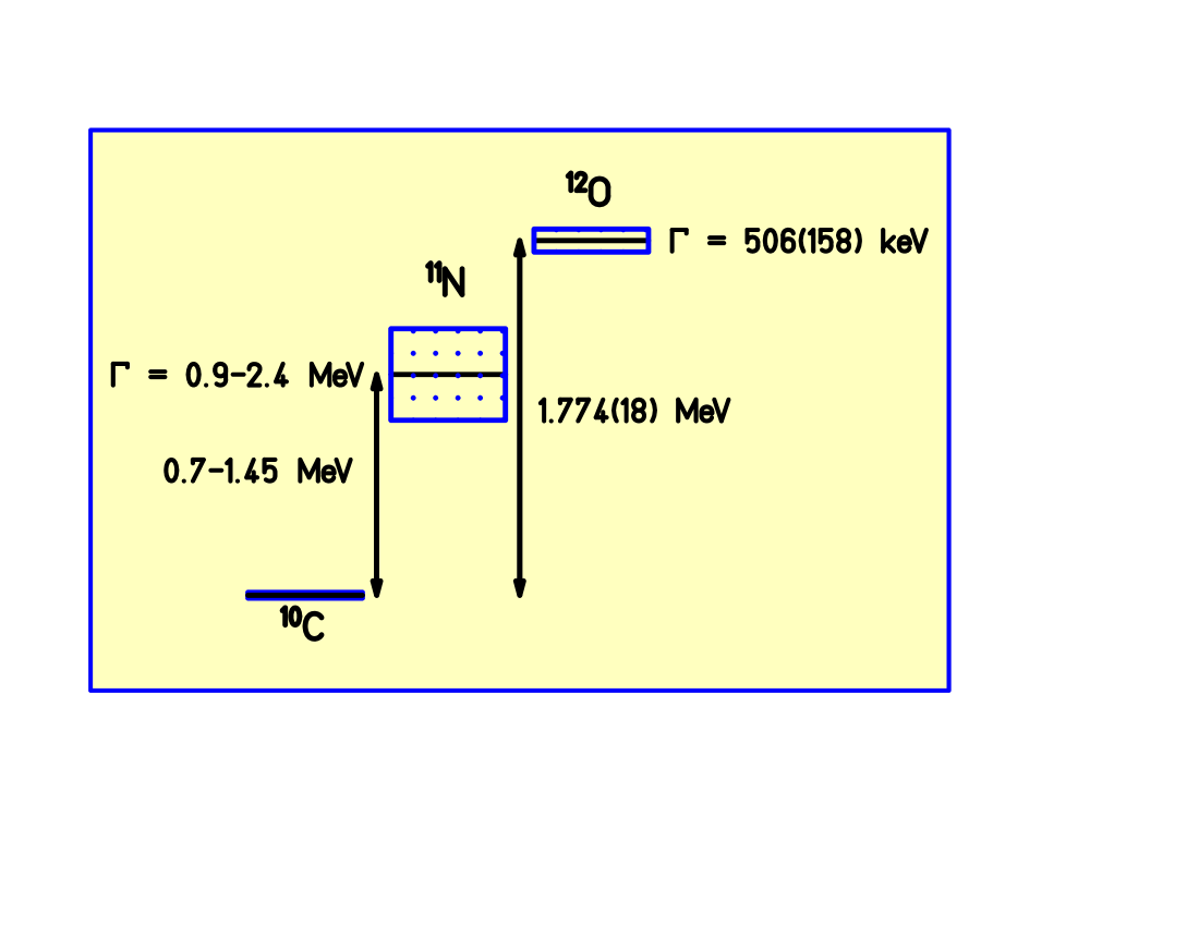
Figure 3: Experimental spectra for the decay of ¹²O and level scheme. The experimental data are compared with Monte-Carlo simulations using the two extreme pictures, i.e. sequential (full line) or diproton (dashed line) decay. Quantitative agreement is obtained within the sequential decay picture. The decay scheme evidences that the sequential path is energetically open [24, 53]. Figures re-used with permission from APS.

These experimental data were interpreted by means of Monte-Carlo simulations, which employed the R-matrix theory [54] to describe the 2p decay in two extreme pictures: diproton emission with a ²He resonance energy of 50 keV and three-body decay which is only restricted by the available phase space. Fig. 3 summarizes these results. A comparison of the experimental results and the simulations clearly favours an uncorrelated three-body emission or a sequential decay, which may have roughly the same characteristics. At the time of this work, these conclusions were somewhat surprising, as it was believed that the intermediate 1p daughter state in ¹¹N was inaccessible due to energy conservation. In addition, a very large ¹²O decay width was needed to explain the experimental data. However, later measurements [55, 56, 57] revealed that the ¹¹N ground state lies lower in mass and opens therefore the way for a sequential decay. With these new results, a consistent description of the decay of ¹²O could be provided [53].

4.3 The decay of ${}^{16}{\rm Ne}$ and ${}^{19}{\rm Mg}$

The decay of ¹⁹Mg was recently studied in an experiment at the fragment separator FRS of GSI [58]. In this experiment, ¹⁹Mg was produced by a one-neutron stripping reaction at the FRS intermediate focal plane of ²⁰Mg, produced itself at the FRS target in a fragmentation reaction of the ²⁴Mg primary beam. The protons emitted in the decay of ¹⁹Mg were detected and tracked by a set of three DSSSD, whereas the heavy decay product, ¹⁷Ne, was identified and its momentum measured in the second half of the FRS.

The measured data were compared to Monte Carlo simulations and allowed to extract the half-life of ¹⁹Mg of $T_{1/2}$ = 4.0(15) ps and the associated two-proton Q-value: $Q_{2p}$ = 0.75(5) MeV. This value is much smaller than standard predictions like the one of the Atomic Mass Evaluation [47] ($Q_{2p}$ = 2.00(25) MeV), the Garvey-Kelson relation [59] ($Q_{2p}$ = 1.02(2) MeV), or the prescription from Antony et al. [60] ($Q_{2p}$ = 1.19(3) MeV). However, the correlation between the Q value and the decay half-life is well reproduced within the three-body model of Grigorenko and co-workers [36].

In the same experiment [58], the decay of ¹⁶Ne by two-proton emission was also observed and the known decay Q value [61] of 1.41(2) MeV was used to test the experimental procedure.

4.4 Conclusions and future studies with short-lived ground-state two-proton emitters

For the systems ⁶Be, ¹²O, and ¹⁶Ne, the decaying states have large widths so that the 2p emitter state and the 1p daughter state overlap. Therefore, the sequential decay channel is opened and the decay will most likely take place sequentially. The situation in the case of ¹⁹Mg is less clear, as the structure and the mass of the one-proton daughter ¹⁸Na is not known. However, with increasing nuclear charge, the Coulomb barrier becomes stronger and the wave function is more and more confined in the nuclear interior which yields narrower states.

Therefore, it might well be that in nuclei like ²¹Si, ²⁶S, or ³⁰Ar the Coulomb barrier is already strong enough so that, with a possibly small decay energy, narrow levels avoid overlapping and the sequential decay path is, at least in a simple picture, not open.

5 Observation of two-proton emission from excited states

Generally speaking, the 2p emission can take place as a sequential-in-time process or a simultaneous process. In its standard form, the sequential process happens when levels in the 1p daughter nucleus, both resonant and non-resonant ones, are accessible for 1p emission. This situation may be encountered when the emission takes place from highly excited levels of the 2p emitter. These levels can be fed either by $\beta$ decay or by a nuclear reactions.

A clear signal for a sequential emission can be obtained when the intermediate level through which the emission passes is identified. This is the case, for example, when well defined one-proton groups sum up to a fixed 2p energy. The one-proton groups give then the energy difference between two well-defined nuclear levels.

5.1 $\beta$-delayed two-proton emission

The possibility of $\beta$-delayed 2p ($\beta$2p) emission was first discussed by Jänecke [14]. He concluded that there should be no ”$\beta$-delayed diproton emitters” with Z$\leq$14. This decay mode was also studied by Goldanskii [62] who proposed possible candidates.

The first experimental observation of $\beta$-delayed 2p emission was reported by Cable et al. in 1983 [25]. Their experiments, using a ³He induced reaction on a magnesium target and a helium-jet technique, led to the first observation of ²²Al by means of its $\beta$-delayed 1p emission from the isobaric analogue state (IAS) in ²²Mg to the ground and first excited states of ²¹Na [63]. The $\beta$2p decay mode was subsequently observed with two silicon detector telescopes which allowed to measure the energy of the two individual protons with good resolution [25].

From the observation of well defined one-proton groups, Cable et al. concluded that this decay is a sequential mode via intermediate states in the 1p daughter nucleus ²¹Na. This conclusion was confirmed in a further experimental study [64] where it turned out that the angular distribution of the two protons is compatible with an isotropic emission, although a small angular correlation (less than 15%) could not be excluded.

Meanwhile more $\beta$2p emitters have been identified. Shortly after the discovery of $\beta$2p decay from ²²Al [25], the same authors observed $\beta$2p emission from ²⁶P [65] and from ³⁵Ca [66]. All in all, nine $\beta$2p emitters have been observed: ²²Al [25], ²³Si [67], ²⁶P [65], ²⁷S [68], ³¹Ar [69], ³⁵Ca [66], ³⁹Ti [70], ⁴³Cr [71, 72], and ⁵⁰Ni [73]. Most of these studies were characterized by rather low statistics inherent to most investigations of very exotic nuclei and hence no detailed search for angular correlations could be performed. In addition, most of the observed decays proceed via the IAS in the $\beta$-decay daughter nucleus. The 2p emission from this state is forbidden by the isospin conservation law and can only take place via a small isospin impurity of the IAS.

The first high-statistics study of a $\beta$2p emitter was carried out at ISOLDE in CERN [74, 75, 76, 77]. For the first time, a rather high-efficiency, high-granularity setup which allows a high-resolution measurement in energy and angle was used. This experiment, which studied the decay of ³¹Ar, demonstrated the occurrence of $\beta$2p decay branches via states other than the IAS. Indeed, many Gamow-Teller fed states could be shown to decay by 2p emission. The main interest of these decays is that they are isospin allowed and cover a wider range of spins for the 2p emitter states, the possible intermediate states and the final states.

Detailed studies of the proton-proton angular correlation for different 2p emission branches did not yield evidence for any angular correlation. In fact, the results were compatible with sequential emission via intermediate states in the 1p daughter nucleus. Although there was some activity detected with the two protons sharing the available decay energy equally, the statistics of these events was too low and the angular coverage of the setup was not uniform enough to draw any conclusion on the possible observation of events, where the protons were correlated in energy and angle. Therefore, despite a factor of 10-100 higher statistics as compared to earlier experiments, no angular and energy correlation, a possible signature of a strong proton-proton correlation, could be evidenced.

This observation is not really astonishing. According to Brown [78], who studied the competition between 1p emission and correlated 2p (diproton) emission from the IAS in ²²Mg, the weight of the direct 2p branch is expected to be at best of the order of a few percent and therefore rather difficult to observe experimentally. New attempts to search for such a correlated 2p emission in ³¹Ar are on the way [79]. These studies take profit from a much more uniform angular coverage.

5.2 Two-proton emission from excited states populated in nuclear reactions

Besides populating excited 2p emitter states by $\beta$ decay, these nuclear states can also be fed by nuclear reactions like pick-up, transfer, or fragmentation. In this section, we will describe experiments which used this kind of interaction to study 2p emission from excited states.

5.2.1 Two-proton emission from ¹⁴O

In an experiment performed at Louvain-La-Neuve, Bain et al. [26] bombarded a (CH₂)_n target with a ¹³N radioactive beam populating highly-excited states in ¹⁴O. The 7.77 MeV state in ¹⁴O, which is strongly populated in 2p transfer reactions [80], is expected to have a significant admixture of a 2p configuration outside of the ¹²C core. In addition, this state is 2p unbound by about 1.2 MeV and, unlike states populated by a super-allowed $\beta$ decay, the 2p decay to the ground state of ¹²C is isospin allowed. Therefore, this resonance was believed to have a small 2p decay branch, either directly to the ¹²C ground state or sequentially via a narrow state in ¹³N (see Fig. 4).

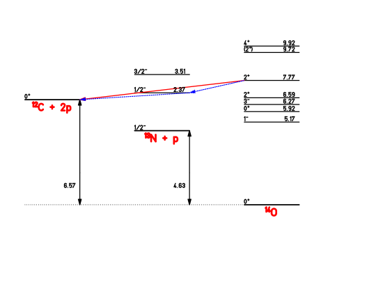
Figure 4: Decay scheme of the 7.77 MeV resonance in ¹⁴O by two-proton emission. A direct decay to the ground state of ¹²C is possible, but the decay was found to be predominantly sequential via an intermediate state at 2.37 MeV in ¹³N.

The two protons from the decay of the 7.77 MeV resonance were detected with the LEDA device [26]. The data showed clearly a resonant structure when the beam energy was ’on-resonance’. The authors determined a 0.16(3)% 2p branch for the decay of this resonance. The individual energies of the two protons could be explained by a sequential decay pattern via the 2.37 MeV state in ¹³N. Monte-Carlo simulations employing R-matrix theory showed that the data could be best explained with a 100% sequential decay pattern.

5.2.2 Two-proton emission from ¹⁷Ne

The decay of excited states of ¹⁷Ne by 2p emission was studied several times in recent years [81, 82, 83]. The first excited state of ¹⁷Ne is 1p bound but unbound with respect to 2p decay by 344 keV and may therefore decay by direct 2p emission to the ground state of ¹⁵O (see Fig. 5). Chromik et al. [81, 82] populated the first excited states of ¹⁷Ne by Coulomb excitation and observed their decay by $\gamma$ de-excitation [81] or in a complete-kinematics experiment [82].

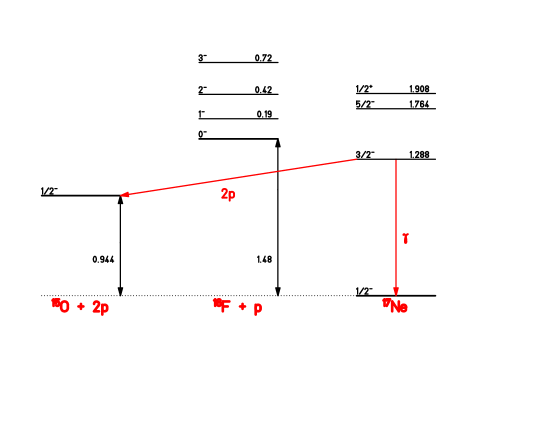
Figure 5: Decay scheme of the excited states in ¹⁷Ne. The first excited state in ¹⁷Ne is bound with respect to one-proton emission but unbound with respect to two-proton emission to the ground state of ¹⁵O. Hence, direct 2p decay is expected. For further details see the discussion in the text.

In the first experiment, the missing strength of the decay of the first excited state by $\gamma$ emission, as compared to theoretical calculations, was interpreted as a possible unobserved 2p branch. However, it was found that such an interpretation was in contradiction to barrier-penetration calculations. In fact, a 2p partial half-life shorter by a factor 1700 than predicted was needed to account for the missing decay strength. The second complete-kinematics experiment allowed determining all decay channels and a partial 2p half-life for the first excited state larger than 26 ps was deduced. No 2p emission from the first excited state was observed. The decay of the second excited state, also populated by Coulomb excitation, was observed to decay by sequential 2p emission to the ground state of ¹⁵O yielding an isotropic emission pattern for the two protons.

This experimental result was confirmed by Zerguerras et al. [83]. In their experiment, excited states of ¹⁷Ne were populated by one-neutron stripping reactions from a ¹⁸Ne beam at 36 MeV/nucleon. States up to 10 MeV excitation energy were observed to decay by 2p emission. The decay products were detected in the MUST detector array [84] and in the SPEG spectrometer [85]. These measurements allowed a reconstruction of the complete decay kinematics and therefore to determine the excitation energy of ¹⁷Ne and the relative proton-proton angle in the center-of-mass frame.

Figure 6: Invariant mass spectrum for ¹⁵O + 2p events [83]. The peak at 18.5 MeV is interpreted as the decay of the second and third excited states of ¹⁷Ne by two-proton emission, whereas the activity above 20 MeV arises from the decay of higher-lying states.

Fig. 6 shows the invariant mass spectrum for ¹⁵O+2p events. The angular distribution of the two protons was measured to be isotropic for the second and third excited states in ¹⁷Ne (Fig. 7a). However, for higher lying states, a distinct angular correlation of the two protons could be observed for the first time (Fig. 7b). This result is rather surprising, as many intermediate states in the 1p daughter nucleus ¹⁶F should be accessible and therefore a sequential decay mechanism via these states should dominate.

The interpretation of this decay pattern is still controversial. Kanungo et al. [86] and Grigorenko et al. [87] suggested that some of the excited states of ¹⁷Ne may have a pronounced 2p halo structure and a large overlap with the ¹⁵O ground state leading to much larger spectroscopic factors for a direct 2p decay than for a sequential decay. Obviously, the validity of this assertion depends on whether the configuration mixing in ¹⁷Ne leaves the ¹⁵O core intact. On the other hand, as shown in SMEC studies [33] the correlated 2p emission is always hindered if 1p decay channels are open. Moreover, the measured energies of the two emitted protons from ¹⁷Ne show large differences which cannot be reconciled with a diproton scenario where roughly equal energies are expected for the two protons.

Another explanation of the 2p emission pattern in ¹⁷Ne could be the large deformation in higher lying states. Strong anisotropy of the Coulomb barrier could be a source of dynamical correlations between emitted protons even if this 2p decay is a sequence of two successive 1p emissions. Effects of this kind have been discussed in the de-excitation of heavy-ion residues (see e.g. Ref. [88]). A similar explanation has been put forward also in connection with the anomalous decay properties of ⁹⁴Ag^m [27]. Obviously, for a consistent interpretation of the ¹⁵O + 2p experiment, higher statistics data is mandatory.

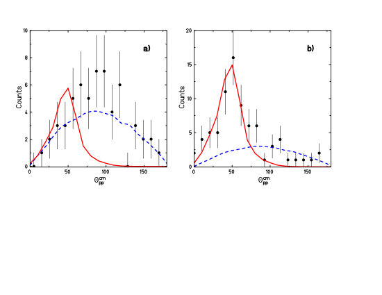
Figure 7: Proton-proton angular distribution for 2p events with a ¹⁵O recoil yielding a mass excess of less than 20.2 MeV (a) and above 20.2 MeV (b) (see Fig. 6). The solid and the dashed curves are simulations of a correlated two-proton emission via a ²He resonance and a sequential emission pattern, respectively [83].

5.2.3 Two-proton emission from ¹⁸Ne

In an experiment performed at ORNL Oak Ridge, Gomez del Campo et al. [89] used a radioactive ¹⁷F beam on a (CH₂)_n target to produce excited states in ¹⁸Ne. The experiment used a thick-target approach, i.e. only the protons could be detected behind the target, whereas the beam-like particles (e.g. the heavy ¹⁶O recoils from the decay of excited states in ¹⁸Ne) could not penetrate the target. Therefore, only protons with a relatively large energy loss depending on their emission point in the target could be observed. Using two different incident energies of the ¹⁷F beam, these authors observed at higher incident energy the emission of two protons which they interpreted as a decay of the 6.15 MeV resonance state in ¹⁸Ne. For the lower energy, where this state could not be populated, no coincident protons were observed. Both the relative proton-proton angle and the energy difference between the two protons was in agreement with simulations for a three-body decay of this state as well as for a diproton-type decay. This lack of sensitivity is to a large extent due to the limited statistics of the experiment, but also due to the limited angular coverage of the experimental setup.

5.2.4 Two-proton emission from ⁹⁴Ag

The decay of ⁹⁴Ag^m is unusual in several respects. It possesses two $\beta$-decaying isomers and has the highest spin state ever observed which decays by $\beta$ decay. In particular, the second isomeric level seems to decay by several different decay branches: $\beta$-delayed $\gamma$ decay [90, 91], $\beta$-delayed proton emission [92], direct proton decay [93], and direct 2p emission [27]. All these experiments were performed at the on-line separator of GSI [94].

The two protons were observed by means of silicon strip detectors which surrounded the implantation point of the on-line separator. This setup allowed for the measurement of the individual proton energies and the relative proton-proton angle. Although the statistics of the 2p experiment is rather low [27], the authors identified proton-proton correlations. They interpreted these data as due to simultaneous 2p emission from a strongly deformed ellipsoidal nucleus. In this case, the asymmetric Coulomb barrier favours the emission of two protons within narrow cones around the poles of the ellipsoid, either from the same pole or on opposite sides.

One should mention, that the observed proton-proton correlations in such a scenario are largely unrelated to the proton-proton correlations inside a nucleus. The microscopic theoretical study of the ⁹⁴Ag^m decay is also impossible using the present-day computers, though only such studies could disentangle an internal structure of decaying states from dynamical effects of the anisotropic Coulomb barrier, providing more details about the 2p decay pattern in the nucleus. Unfortunately, further experimental studies of the ⁹⁴Ag^m decay cannot be made without new technical developments to produce ⁹⁴Ag^m, as the on-line separator of GSI has been dismantled a few years ago.

6 Two-proton radioactivity

Goldanskii [1, 11] called it a pure case of 2p radioactivity, if 1p emission is not possible because the 2p emitter level is lower in energy than the level in the 1p daughter nucleus and, moreover, the corresponding levels are sufficiently narrow and thus do not overlap. The limitations of this picture will be discussed in chapter 8. Goldanskii also gave an arbitrary half-life limit of 10^-12 s [95] to distinguish between two-proton radioactivity and the decay of particle-unstable nuclei. None of the examples discussed above satisfy Goldanski’s radioactivity criterion; they all have rather short half-lives (of the order of 10^-21 s) and for the light ground-state emitters, the states which emit the first and the second proton overlap significantly. In this sense, 2p radioactivity was observed for the first time in ⁴⁵Fe experiments [19, 20]. Later ⁵⁴Zn [21] and possibly ⁴⁸Ni [22] were shown to be other ground-state 2p emitters.

Recent theoretical predictions [15, 17, 16] agree that ³⁹Ti, ⁴²Cr, ⁴⁵Fe, and ^49,48Ni are candidates to search for 2p radioactivity. Firstly, their predicted decay energy is close to or in the range of energies (1.0-1.5 MeV) where 2p radioactivity is most likely expected to occur, and secondly these isotopes are already or could soon be produced in projectile-fragmentation type experiments. This production technique allows to unambiguously identify the isotopes before their decay and thus measure the decay half-life and the decay energy, the necessary ingredients to identify this new radioactivity. The most promising candidates were ⁴⁵Fe and ⁴⁸Ni with decay energies of 1.1-1.4 MeV.

6.1 Identification of the 2p candidates and first negative results

The first of these isotopes, ³⁹Ti, was observed at the Grand Accélérateur National Ions Lourds (GANIL), Caen [96] in 1990. This experiment was also the first attempt to observe 2p radioactivity of these medium-mass nuclei after projectile fragmentation. However, no indication for 2p radioactivity could be found. Instead, a $\beta$-decay half-life of 28${}^{+8}_{-7}$ms was measured and $\beta$-delayed protons were observed. Another attempt to search for 2p radioactivity from ³⁹Ti was made at GANIL in 1991 with an improved setup [97, 98]. However, again no 2p events could be observed.

The nuclei ⁴²Cr, ⁴⁵Fe, and ⁴⁹Ni were identified for the first time a few years later at GSI [99]. In this experiment, no spectroscopic studies could be performed and the observation of these isotopes was the only outcome. Nonetheless, this experiment provided the first observation of one of the most promising 2p radioactivity candidates and opened the door for the search of ⁴⁸Ni, another candidate. This doubly-magic nucleus was then discovered in 1999 [100] in a GANIL experiment using the SISSI/LISE3 device [101]. In the same experiment, the observation of ⁴⁵Fe was confirmed with about a factor of 10 higher statistics.

The GANIL experiment was also set up to perform spectroscopic studies of the very exotic nuclei produced [102]. The decay trigger in this experiment allowed mainly $\beta$-delayed events to be registered. $\beta$-delayed decay events from e.g. ⁴⁵Fe decay had a detection efficiency of about 30%, as they were triggered by two detectors adjacent to the implantation detector. 2p events without $\beta$ particle had a very low trigger rate (a few percent) due to a heavy-ion trigger for the implantation device. This situation allowed for the observation of the decay of ⁴⁵Fe, however, basically of only its $\beta$-delayed branch (see Sect. 6.2). In any case, no claim about the observation of 2p radioactivity was made.

Nevertheless, the experiment allowed one to test two other possible, although less promising, 2p candidates: ⁴²Cr and ⁴⁹Ni. As mentioned above, these two nuclei were predicted to be possible 2p emitters, however, with decay energies most likely too small to exhibit this decay. The decay energy spectrum obtained during this experiment for ⁴²Cr is shown in Fig. 8. The prominent peak at 1.9 MeV was excluded to be of 2p nature, as such a high energy would lead to an extremely short barrier penetration time for the two protons (see Fig. 8, right-hand side), in contradiction with the ⁴²Cr half-life of 13.4${}^{+3.6}_{-2.4}$ms measured in the same experiment.

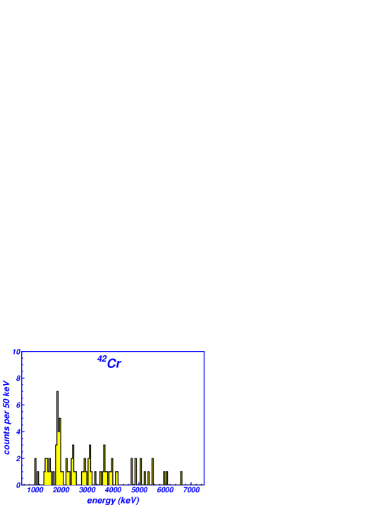
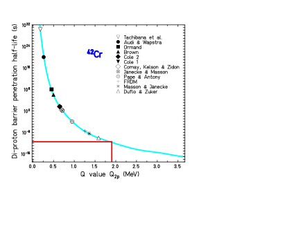
Figure 8: Left-hand side: Charged-particle decay-energy spectrum obtained after ⁴²Cr implantation. The 1.9 MeV peak is interpreted as a $\beta$-delayed decay [102]. Right-hand side: Barrier penetration half-life for a di-proton in ⁴²Cr as a function of the available decay energy [102]. The red line represents the 1.9 MeV peak from the decay-energy spectrum yielding a barrier penetration half-life of 10^-12s if it were of 2p origin.

In a similar way, ⁴⁹Ni could be excluded from having a significant direct 2p branch. The last 2p emitter candidate tested in this experiment was ³⁹Ti. In agreement with previous experiments, this nucleus turned out to decay predominantly by $\beta$ decay. Several $\beta$-delayed proton groups could be identified and the 2p emission Q value (Q_2p = 670$\pm$100 keV) could be determined, indicating a rather high barrier-penetration half-life and therefore a rather low probability for 2p radioactivity.

6.2 The discovery of two-proton radioactivity

The discovery of ground-state 2p radioactivity had to await the year 2002, when two experiments, one performed in 2000 at the SISSI/LISE3 facility of GANIL [19] and one performed at the FRS of GSI in 2001 [20], were published. Both experiments used the fragmentation of a ⁵⁸Ni primary beam. The fragments of interest were implanted in a silicon detector telescope (see Fig. 9), where correlations in time and space between implantation events and decay events could be performed. This technique allowed to unambiguously correlate ⁴⁵Fe implantation events with their decays.

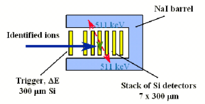
Figure 9: Left-hand side: Detection setup used in the GANIL experiment to identify two-proton radioactivity. The setup consisted of a silicon telescope, where the implantation device was a double-sided silicon strip detector (DSSSD). Several time-of-flight, energy-loss and residual energy measurements allowed an unambiguous identification of the projectile fragments. The radioactive decay of the isotopes of interest was detected in the DSSSD. The last detector, a Si(Li) detector, was used to detect $\beta$ particles [19]. Right-hand side: Setup used in the GSI experiment. A silicon telescope of seven elements was surrounded by a high-efficiency NaI array. Implantation and decay events were correlated in different detectors depending of the implantation depth of the ⁴⁵Fe ions. The NaI device served to search for $\gamma$ radiation from positron annihilation [20].

Fig. 10 shows the decay energy spectra from the two experiments. Both find a decay energy of about 1.1 MeV with a decay half-life in the 3-5 ms range. An additional feature of both experiments was the capability to detect additional radiation like $\beta$ particle in the GANIL experiment, or 511 keV annihilation radiation and other $\gamma$ rays in the GSI experiment (see Fig. 9). This capability allowed for a rejection with a high probability of a possible $\beta$-delayed origin of the decay events with an energy release of about 1.1 MeV. Other pieces of evidence from the GANIL experiment were the smaller width of the 1.14 MeV peak as compared to $\beta$-delayed proton emission peaks in neighbouring nuclei and the observation of daughter decays consistent with the decay of ⁴³Cr, the 2p daughter of ⁴⁵Fe. In addition, the experimentally observed decay energy is in nice agreement with theoretical predictions [15, 17, 16]. These experimental results led the authors to conclude the discovery of ground-state 2p radioactivity in the decay of ⁴⁵Fe.

Of particular interest was also the observation of decay events from ⁴⁵Fe with an energy release different from the 1.1 MeV of the main peak. Some of these additional events could be identified as being in coincidence with $\beta$ particles and were therefore attributed to $\beta$-delayed decay branches. From these first results, a 2p radioactivity branching ratio of 70-80% was determined for ⁴⁵Fe. The partial half-lives of ⁴⁵Fe for 2p emission and for $\beta$ decay are therefore of the same order and allowed the two decay modes to compete.

These results on ⁴⁵Fe have recently been confirmed in a new GANIL experiment [22]. Several experimental improvements allowed a better energy calibration and a smaller data acquisition dead time. The decay energy was determined to be 1.154(16) MeV, the half-life to be 1.6${}^{+0.5}_{-0.3}$ms, and the 2p branching ratio to be 57(10)%. Together with the results from the two earlier experiments [19, 20], this experiment allowed to determine average values for the decay energy (Q_2p= 1.151(15) MeV), the half-life (T_1/2= 1.75${}^{+0.49}_{-0.28}$ms), the 2p branching ratio (BR = 59(7)%), and the partial 2p half-life (T${}_{1/2}^{2p}$= 3.0${}^{+0.9}_{-0.6}$ms).

In 2007, a new experiment performed at the A1900 separator of Michigan State University allowed the observation of 2p events in a TPC (see below). The newly determined half-life and the 2p branching ratio are included in Table 1 to determine average values. These average values will be used in the comparison with theoretical model of 2p radioactivity.

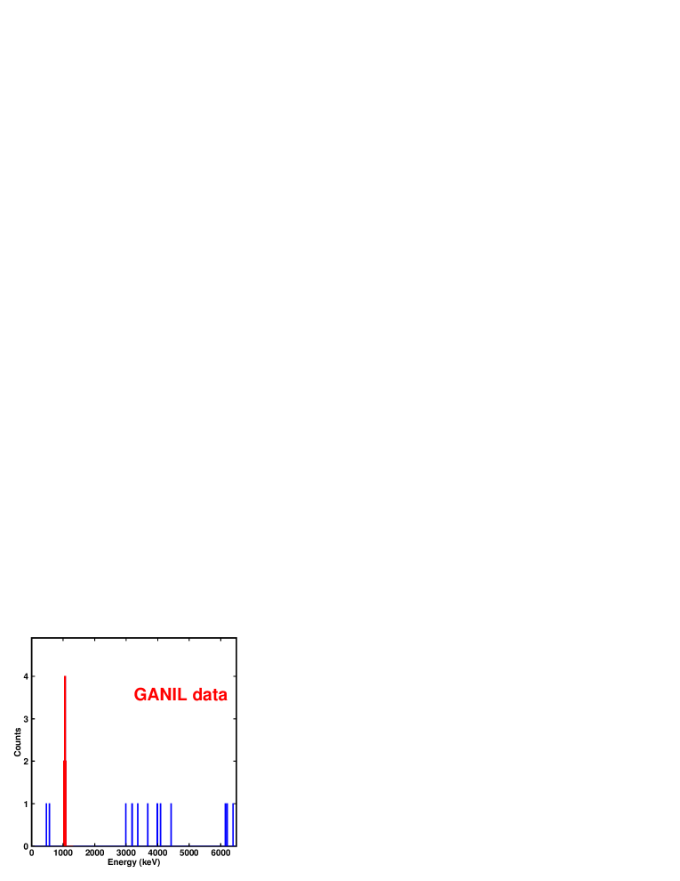
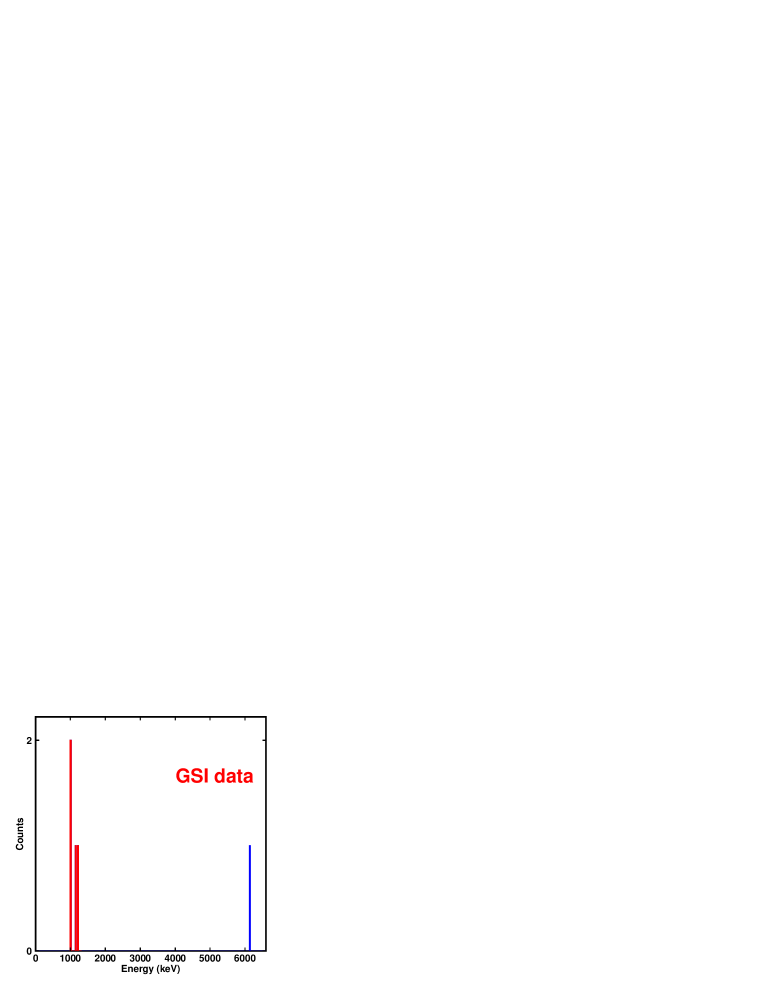
Figure 10: Left-hand side: ⁴⁵Fe decay-energy spectrum from the GANIL experiment exhibiting a peak at (1.14$\pm$0.04) MeV [19]. Right-hand side: ⁴⁵Fe decay-energy spectrum from the GSI experiment showing four events at 1.1(1) MeV [20]. Both spectra also show events at higher energies.

Another outcome from the GANIL experiments [19, 22] on ⁴⁵Fe was the determination of the half-life of the 2p daughter nucleus. From the observation of the second decay after ⁴⁵Fe implantation, the half-life of the daughter decay, in coincidence with the 1.151 MeV peak, could be determined. In Fig. 11, this half-life is compared to the half-lives of all possible ⁴⁵Fe daughter nuclei. Only the half-life of ⁴³Cr is in agreement with the experimentally observed daughter half-life, thus giving an independent proof for the observation of 2p radioactivity.

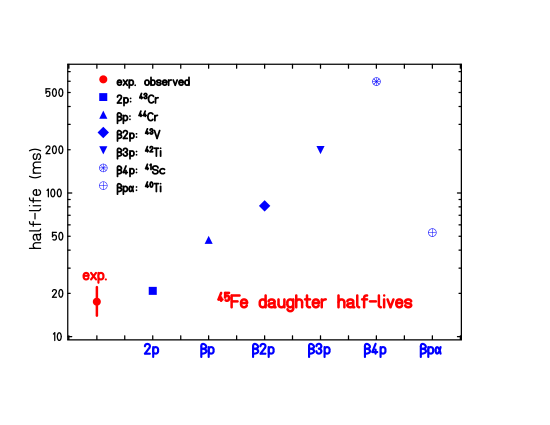
Figure 11: The experimentally observed half-life for the decay of the daughter of ⁴⁵Fe is compared to the half-lives of all possible daughters [73]. Only the half-life of ⁴³Cr is in agreement with the experimental value.

6.3 Two-proton radioactivity of ⁵⁴Zn

The nucleus ⁵⁴Zn was early identified as a possible 2p emitter [10, 11]. More recent $Q_{2p}$ estimates yielded decay energies of 1.79(12) MeV [16], 1.87(24) MeV [103], and 1.33(14) MeV [104]. Due to rather large theoretical error bars and the uncertainty concerning the decay mechanism, it was rather unclear whether ⁵⁴Zn would exist at all, i.e. whether its half-life would be long enough to be observed in projectile-fragmentation type experiments. For this purpose, a life time of the order of a few hundred nano-seconds was mandatory.

The search for ⁵⁴Zn began with the observation of two other proton-rich zinc isotopes, ⁵⁶Zn and ⁵⁵Zn [105]. They were observed for the first time in experiments at the LISE3 separator [101] via 2p pick-up reactions with a ⁵⁸Ni primary beam. The identification of these two isotopes allowed also for an extrapolation of the production cross section of ⁵⁴Zn.

The nucleus ⁵⁴Zn was synthesized and observed for the first time in 2004 in an experiment at the SISSI/LISE3 facility of GANIL Caen [21]. Similarly to the experiment with ⁴⁵Fe, ⁵⁴Zn was produced with a primary ⁵⁸Ni beam at 75 MeV/nucleon impinging on a natural nickel target. The fragments of interest were selected and separated with the LISE3 separator and implanted in a silicon telescope with a double-sided silicon strip detector being the central device. The ⁵⁴Zn nuclei were identified by means of time-of-flight, energy-loss and residual-energy measurements. Fig. 12 shows the two-dimensional identification plot for the ⁵⁴Zn experiment. All in all, eight ⁵⁴Zn nuclei could be unambiguously identified.

Figure 12: Two-dimensional identification plot for ⁵⁴Zn and neighbouring nuclei. The energy loss in the first silicon detector of the detection setup is plotted as a function of the time-of-flight through the separator. Additional parameters are used to purify the spectrum [21].

The setup allowed correlating in time and space these implantation events with subsequent decays. Seven of the eight implantation events are followed by a decay with an energy release of 1.48(2) MeV (see Fig. 13). None of these decay events is in coincidence with a $\beta$ particle. As for ⁴⁵Fe, the 1.48 MeV peak is much narrower than $\beta$-delayed proton lines in neighbouring nuclei. Although less significant

Figure 13: Charged-particle spectrum from the decay of ⁵⁴Zn. The peak at 1.48(2) MeV is due to two-proton emission from the ground state of ⁵⁴Zn. The event at 4.19 MeV is in coincidence with a $\beta$ particle in the adjacent detector [21].

as in the case of ⁴⁵Fe, daughter decays in agreement with the decay of ⁵²Ni, the 2p daughter of ⁵⁴Zn, could be observed. Finally, the experimental half-life (T_1/2= 3.2${}^{+1.8}_{-0.8}$ms) is in agreement with what is expected for a 2p decay with an energy release of 1.48 MeV. From these experimental observations, the authors concluded the observation of ground-state 2p radioactivity from ⁵⁴Zn. The 2p branching ratio was determined to be 87${}^{+10}_{-17}$%, which yielded a partial half-life for 2p decay of 3.7${}^{+2.2}_{-1.0}$ ms. These results will be compared to theoretical predictions in Sect. 9.3.

6.4 The decay of ⁴⁸Ni

The discovery of ⁴⁸Ni and the observation of its decay was considered important for several reasons. Firstly, it is a doubly-magic nucleus which was predicted to be particle stable or quasi-stable only due to strong shell effects. Secondly, ⁴⁸Ni is one of the most exotic of all doubly-magic nuclei within experimental reach. Its observation and the measurement of its properties, like e.g. the excitation energy of the first 2⁺ state, were expected to teach us a lot about the persistence of shell structure far from the valley of stability.

The nucleus ⁴⁸Ni was rather early identified as a possible 2p emitter [1]. This prediction was confirmed and refined by new mass and $Q_{2p}$ calculations, which yielded 1.36(13) MeV [15], 1.14(21) MeV [17], 1.35(6) MeV [16], and 1.29(33) MeV [103]. When compared to ⁴⁵Fe and ⁵⁴Zn, it is evident that this $Q_{2p}$ value is again in the right range to permit ⁴⁸Ni to have a significant 2p radioactivity decay branch.

The isotope ⁴⁸Ni was first observed in 1999 at GANIL Caen [100], where four events could be unambiguously identified. This result was confirmed in 2004, when again four events of ⁴⁸Ni could be registered in a new SISSI/LISE3 experiment at GANIL [22]. These data were obtained in the same run as the second ⁴⁵Fe data set from GANIL, because the acceptance of the SISSI/LISE3 device allows the measurement of different neighbouring nuclei at the same time. Fig. 14 shows the fragment identification plot.

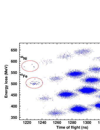
Figure 14: Two-dimensional identification plot for ⁴⁸Ni and neighbouring nuclei. The energy loss in the first silicon detector is plotted as a function of the flight time through the separator. Additional parameters are used to purify the spectrum [22].

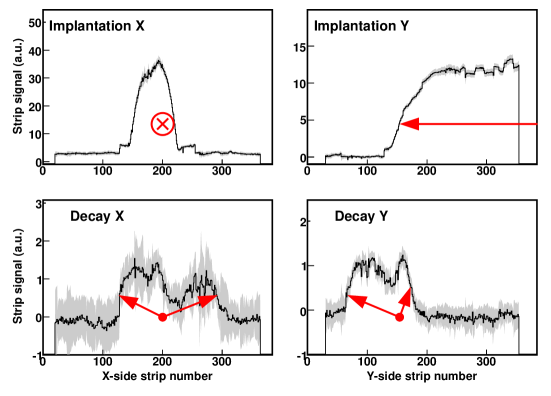
Figure 15: A single event of two-proton decay of ⁴⁵Fe from a recent experiment performed with the Bordeaux TPC at the LISE3 facility of GANIL [72]. The top row shows the ⁴⁵Fe implantation event, where the ion enters the chamber parallel to the X direction and stops in the center of the chamber. The decay (bottom) takes place at the point where the ion stopped.

The four ⁴⁸Ni implantation events could be correlated in time and space with subsequent decay events. From the four decay events, only one event has all characteristics of a 2p emission: a decay energy of 1.35(2) MeV in the expected energy range and no coincident $\beta$ particle. The decay takes place after 1.66 ms and the daughter decay is also fast as expected for ⁴⁶Fe, the 2p daughter of ⁴⁸Ni. These four decay events, one of possible 2p origin and three from $\beta$-delayed decays, were also used to determine the half-life of ⁴⁸Ni (T_1/2= 2.1${}^{+2.1}_{-0.7}$ms). Although this single possible 2p decay event is not considered sufficient to claim the observation of 2p radioactivity for ⁴⁸Ni, these data were nonetheless used to determine the 2p branching ratio to be 25${}^{+29}_{-19}$% and the partial 2p half-life to be T${}_{1/2}^{2p}$=8.4${}^{+12.8}_{-~{}7.0}$ms [22].

6.5 Direct observation of two protons in ground-state decay of ⁴⁵Fe

From all 2p emitters observed up to now, the ground-state emitter ⁴⁵Fe is the best candidate to search for a clear signal of correlated emission and to study in detail the decay mechanism.

As just mentioned, 2p emission could only be governed by phase space or there could be more or less strong angular and energy correlations. In order to study these questions, new experimental setups had to be imagined, the basic limitation of the silicon-detector setups being that the 2p emitters are deeply implanted in a silicon detector, which then does not allow the detection of individual protons, but rather of the total decay energy and the half-life only.

The solution to this problem is the use of gas detectors capable to visualize the traces of the emitted protons. Therefore, time projection chambers (TPC) were set up in Bordeaux [106] and Warsaw [107]. The Bordeaux detector is based on gas electron multiplier technology [108] and a double-sided microgroove detector [109] with an application-specific integrated-circuit read-out, whereas the Warsaw detector uses an optical read-out system by means of a digital camera and a photomultiplier tube (PMT) which registers the time sequence. Both TPC detectors have recently taken first data [72, 110] (see Figs. 15, 16). Due to the highest production rates, ⁴⁵Fe was the first 2p emitter to be studied with these devices.

Due to the higher statistics, the data taken at Michigan State University with the Warsaw TPC allowed to compare the experimental data to predicitons of the ${\rm S}\ell^{2}{\rm M}$ model of Grigorenko et al. model [111], for which nice agreement for the angular and energy distribution was reached [110] indicating e.g. an equal sharing of the energy between the two protons.

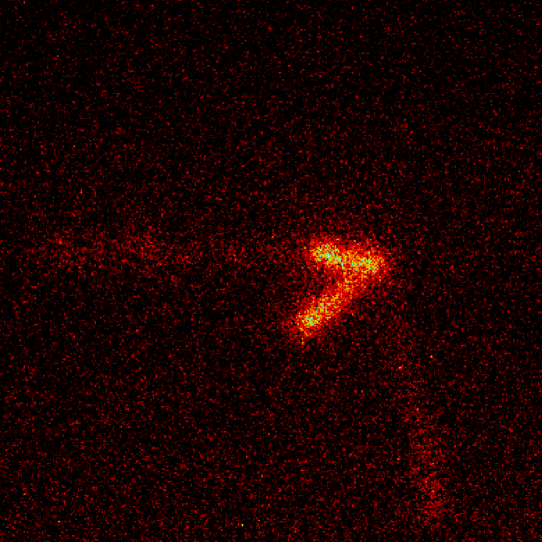
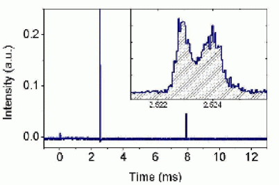
Figure 16: An example of a two-proton decay event of ⁴⁵Fe recorded by the Warsaw TPC detector. Left: an image taken by the CCD camera in a 25 ms exposure. The faint track of a ⁴⁵Fe ion entering the chamber from the left is seen. The two bright, short tracks are low-energy protons emitted approximately 2.5 ms after the implantation. A weaker and longer track, going from the decay vertex to the lower right, represents a high-energy proton emitted about 8 ms after the implantation which is due the decay of ⁴³Cr, the 2p decay daughter of ⁴⁵Fe. Right: the time profile of the total light intensity, measured by the PMT, provides the time sequence of the decay events. In the inset, a magnified part is plotted showing in detail the 2p emission. Figure courtesy of M. Pfützner.

7 Conclusion for the experimental part

The observation of ground-state 2p radioactivity for ⁴⁵Fe, ⁵⁴Zn and possibly for ⁴⁸Ni allowed this type of radioactivity to be established as a new nuclear decay mode. Although only based on theoretical mass predictions, these decays are believed to be simultaneous emissions of the two protons. A sequential decay could have a sizable contribution only if the $Q_{1p}$ values were off by a few hundred keV what is rather unlikely. Nonetheless, the assumption that the decay is indeed simultaneous still awaits experimental verification though, as will be discussed in Sect. 9, a symmetric energy distribution of individual protons emitted in the 2p decay of ⁴⁵Fe [110] is a strong indication for a predominance of the simultaneous 2p emission. Table 1 summarizes the experimental information available for ⁴⁵Fe, ⁴⁸Ni, and ⁵⁴Zn.

	2p decay energy	half-life	branching ratio	partial half-life
	(MeV)	(ms)		(ms)
45Fe	1.151$\pm$0.015	2.5${}^{+0.2}_{-0.2}$	0.65$\pm$0.05	3.9${}^{+0.4}_{-0.4}$
48Ni	1.35$\pm$0.02	2.1${}^{+2.1}_{-0.7}$	0.25${}^{+0.29}_{-0.19}$	8.4${}^{+12.8}_{-7.0}$
54Zn	1.48$\pm$0.02	3.2${}^{+1.8}_{-0.8}$	0.87${}^{+0.10}_{-0.17}$	3.7${}^{+2.2}_{-1.0}$

Table 1: Decay energies, half-lives, branching ratios, and partial half-lives as determined in three independent experiments for the decay of ⁴⁵Fe [19, 20, 22, 110] as well as for ⁴⁸Ni [22], and ⁵⁴Zn [21].

To get a coherent picture of this new decay mode, more 2p emitters have to be studied experimentally. However, as these nuclei are, by definition, situated beyond the proton drip line, their production is rather difficult and the rates are very low. Rather high rates can be achieved today at the SISSI/LISE3 facility of GANIL with about 10-15 ⁴⁵Fe per day, about 2 ⁵⁴Zn per day, and roughly 1 ⁴⁸Ni per day under optimal conditions. It was recently shown that at the coupled-cyclotron facility and the A1900 separator of the NSCL even higher rates can be achieved. Other candidates like ⁵⁹Ge, ⁶³Se or ⁶⁹Kr might be reached in the near future at the new RIKEN Radioactive Ion Beam Facility (RIBF) in Tokyo, Japan.

8 Theoretical description of two-proton radioactivity

The nuclear many-body Hamiltonian is supposed to describe all nuclei that can exist and not merely one nucleus of a given number of protons and neutrons. In this sense, a nucleus is never a closed, isolated quantum system but communicates with other nuclei through virtual excitations, decays and captures. The communication is broken and the nucleus becomes artificially closed if the subspace of continuum states is excluded in the network of coupled systems. Obviously, the closed quantum system idealization of a real many-body system has very different features from those observed [32, 112], in particular in the neighborhood of each reaction threshold [113, 114].

Most of the nuclear states are embedded in the continuum of decay channels due to which they get a finite lifetime. The initial impulse for a mathematical formulation of the shell model (SM) for open quantum systems goes back to Feshbach and Fano [115, 116, 117] who introduced the two subspaces of Hilbert space: (i) the subspace of discrete states, and (ii) the subspace of real-energy scattering states, respectively. Feshbach achieved a unified description of direct processes at the short-time scale and of compound nucleus processes at the long-time scale [115, 116]. A unified description of both nuclear structure and nuclear reactions in a single theoretical framework became possible only in the continuum SM [118, 119, 120, 121, 122, 123].

First realistic studies using the continuum SM have been presented only at the turn of the century in the framework of SMEC [30, 31] (see also Ref. [32] for a recent review). This model is based on the completeness of the single-particle basis consisting of bound orbits and a real-energy scattering continuum. Single-particle resonances are regularized, i.e. they are included in a discrete part of the spectrum after removing scattering tails which are incorporated in the embedding continuum. Subsequently, the new set of discrete states and the non-resonant scattering states are reorthogonalized. Configuration mixing in the valence space (the internal mixing) is given by an effective SM interaction. Coupling of discrete states to the continuum of decay channels is calculated microscopically and leads to the so-called external mixing of SM wave functions. The decay channels are obtained in the $S$-matrix (scattering-matrix) formalism (see Ref. [32] and references quoted therein).

Another approach referring to the continuum SM has been proposed recently in Refs. [124, 125]. Internal mixing in this approach is given by an effective SM Hamiltonian but an external mixing is neglected. This scheme has been applied to the description of observables in the one- and two-particle continuum [125].

The genuine three-body decay models for 2p radioactivity have been proposed in Refs. [126, 127, 128, 129] using the hyperspherical harmonics method. These models combine the cluster model description of the decaying system with a treatment of three-body asymptotic states of charged particles. Rigorous treatment of a three-body kinematics in these models allows to study both angular and energy/momentum correlations between decaying fragments.

A different approach for describing many-body open quantum systems is provided by a generalization of SM in the complex-momentum plane (the GSM) [130, 35, 131]. This general formalism with no restriction on the number of particles in the scattering continuum has not yet been applied for a description of experimentally observed 2p decays.

8.1 Shell Model Embedded in the Continuum with one particle in the scattering continuum

A general theory of the decaying many-body system is provided by the open quantum system formulation of the SM. Before we turn to the description of 2p decay, let us introduce the basic features of SMEC in the simpler case of the one-particle continuum. In SMEC, the function space consists of two sets: the space of ${\cal L}^{2}$-functions, as in the nuclear SM, and the space of scattering states (decay channels) embedding SM states. The decay is a result of the coupling between discrete states and decay channels. These two sets of wave functions are found by solving the Schrödinger equation for discrete states:

$$H_{SM}|\Phi_{i}\rangle=E_{i}^{(SM)}|\Phi_{i}\rangle~{}\ ,$$ (1)

where $H_{SM}$ is the SM Hamiltonian, and for scattering states:

$$\sum_{c^{\prime}}(E-H_{cc^{\prime}})\xi_{E}^{c^{\prime}(+)}=0~{}\ ,$$ (2)

where $H_{cc}=H_{0}+V_{cc}$ in (2) is the standard coupled-channel Hamiltonian. Different channels are defined by coupling the motion of an unbound particle relative to the residual nucleus with $(A-1)$ particles in a discrete SM state $|\Phi_{j}^{A-1}\rangle$. $\xi_{E}^{c(+)}$ are scattering states projected on the channel $c$, and the channel numbers $c$ are defined by the quantum numbers of of the states $j$ of the residual nucleus and those of the unbound particle which are coupled to the total quantum numbers $J^{\pi}$ and $T$ of the system.

Using these two function sets: ${\cal Q}\equiv\{\Phi_{i}^{A}\}$, ${\cal P}\equiv\{\xi_{E}\}$, one defines projection operators:

$${\hat{Q}}=\sum_{i=1}^{N}|\Phi_{i}^{A}\rangle\langle\Phi_{i}^{A}|~{}~{}~{}~{};~{}~{}~{}~{}~{}{\hat{P}}=\int_{0}^{\infty}dE|\xi_{E}\rangle\langle\xi_{E}|$$ (3)

satisfying ${\hat{Q}}|\xi_{E}\rangle=0$, ${\hat{P}}|\Phi_{i}^{A}\rangle=0$, and projected Hamiltonians: ${\hat{Q}}H{\hat{Q}}\equiv H_{QQ}$ and ${\hat{P}}H{\hat{P}}\equiv H_{PP}$. The closed system Hamiltonian $H_{QQ}$ is the nuclear SM Hamiltonian $H_{SM}$, whereas $H_{PP}$ is given by $H_{cc}$. To construct a complete solution in ${\cal Q}+{\cal P}=I_{d}$:

$$|\Psi_{E}\rangle={\hat{Q}}|\Psi_{E}\rangle+{\hat{P}}|\Psi_{E}\rangle~{}\ ,$$

one has to find a wave function connecting ${\cal Q}$ and ${\cal P}$ subspaces. This wave function $\omega_{i}^{(+)}$ is obtained as a solution of non-homogeneous coupled-channel equations:

$$|\omega_{i}^{(+)}(E)\rangle=G_{P}^{(+)}(E)|w_{i}\rangle~{}\ ,$$ (4)

where $|w_{i}\rangle=H_{PQ}|\Phi_{i}\rangle$ is the source term,

$$G_{P}^{(+)}(E)=\lim_{\epsilon\to 0}[E+i\epsilon-H_{PP}]^{-1}$$

is the Green’s function in ${\cal P}$ subspace, $E$ is the total energy of the nucleus $[A]$, and $H_{PQ}\equiv{\hat{P}}H{\hat{Q}}$. Using the three function sets: $\{\Phi_{i}^{A}\}$, $\{\xi_{E}\}$, and $\omega_{i}^{(+)}(E)$, one can find the solution in the total function space:

$$|\Psi_{E}\rangle=|\xi_{E}\rangle+\sum_{i,k}(|\Phi_{i}^{A}\rangle+|\omega_{i}^{(+)}(E)\rangle)\langle\Phi_{i}^{A}|(E-{\cal H}_{QQ}(E))^{-1}|\Phi_{k}^{A}\rangle\langle\Phi_{k}^{A}|H_{QP}|\xi_{E}\rangle~{}\ .$$ (5)

${\cal H}_{QQ}(E)$ is the energy-dependent effective Hamiltonian in the function space of discrete states:

$${\cal H}_{QQ}(E)=H_{QQ}+H_{QP}G_{P}^{(+)}(E)H_{PQ}$$ (6)

which takes into account couplings to decay channels. In that sense, ${\cal H}_{QQ}$ is the open quantum system Hamiltonian in ${\cal Q}$ subspace.

The second term on the right-hand side of Eq. (6) provides an imaginary part of energy eigenvalues for states above the particle emission threshold. The real part of this term contributes to the real part of energy eigenvalues both below and above the threshold. For that reason, it would be more appropriate in phenomenological applications to fit matrix elements of ${\cal H}_{QQ}$ and not of $H_{QQ}$ to nuclear spectra in a given mass region. This ambition task has not yet been accomplished.

Energies $E_{i}$ and widths $\Gamma_{i}$ of the resonance states derive from the solutions of fixed-point equations:

$$E_{i}={\tilde{E}}_{i}(E=E_{i})~{}~{}~{}~{};~{}~{}~{}~{}\Gamma_{i}={\tilde{\Gamma}}_{i}(E=E_{i})$$ (7)

where functions ${\tilde{E}}_{i}(E)$ and ${\tilde{\Gamma}}_{i}(E)$ follow from (complex) eigenvalues of ${\cal H}_{QQ}$.

The eigenvalues of ${\cal H}_{QQ}$ have a physical meaning if the total function space is divided into the subspaces of the system (the subspace ${\cal Q}$) and the environment (the subspace ${\cal P}$) as follows: the system contains all resonance-like phenomena while the environment describes the smooth part in the energy region considered. This operational definition of subspaces implies that in SMEC one has to construct carefully the single-particle basis. The narrow single-particle resonances in the continuum are included into the set of discrete states either as resonance anamneses [132] or as quasi-bound single-particle states [133]. The new definition of discrete single-particle states implies a redefinition of the continuous spectrum, as described in Ref. [32].

8.2 Theory of two-proton radioactivity

The description of Borromean (halo) systems and two-nucleon decays involves couplings to the two-nucleon decay channels. In the 2p decay, since two protons do not form a bound two-particle system, one neither can uniquely specify the final state of two protons nor the transition path leading to this state. Various transition paths may interfere making distinction between different decay mechanisms difficult if not impossible. In this respect, the 2p decay is qualitatively different from any standard two-body decays such as the proton-, neutron- or $\alpha$-particle decays.

A generalization of the SMEC formalism for larger number of particles in the scattering continuum is conceptually similar to the one-particle case discussed above (cf Sect. 8.1). For the description of two-particle continuum, one has to introduce a subspace ${\cal T}$ with two particles in the continuum, and ${\hat{T}}$ the corresponding projection operator. The completeness relation in total function space is then: ${\cal Q}+{\cal P}+{\cal T}=1$. Similarly as in Sect. 8.1, one can decompose the Hamiltonian $H$ into components acting in different subspaces and the coupling terms between those different subspaces. The ${\cal Q}$ subspace effective Hamiltonian ${\cal H}_{QQ}(E)$ can be written as [34]:

$${\cal H}_{QQ}(E) = H_{QQ}+H_{QP}G_{P}^{+}(E)H_{PQ}$$ (8)

$$+ [H_{QT}+H_{QP}G_{P}^{+}(E)H_{PT}]\tilde{G}_{T}^{+}(E)[H_{TQ}+H_{TP}G_{P}^{+}(E)H_{PQ}]$$

The first term on the right-hand side is the closed quantum system Hamiltonian, the second term describes a coupling with the one-particle continuum, and the third term corresponds to all possible couplings with the two-particle continuum. $\tilde{G}_{T}^{+}(E)$ is the Green function in ${\cal T}$

$$\tilde{G}_{T}^{+}(E)=\lim_{\epsilon\to 0}[E+i\epsilon-H_{TT}-H_{TP}G_{P}^{+}(E)H_{PT}]^{-1}$$

modified by couplings to ${\cal P}$. Similarly as in the case of one-particle continuum, one defines the source term

$$|w_{i}\rangle=[H_{TQ}+H_{TP}G_{P}^{(+)}(E)H_{PQ}]|\Phi_{i}\rangle$$ (9)

and the continuation $|\omega^{+}_{i}\rangle$ of SM wave function $|\Phi_{i}\rangle$ into the two-particle continuum:

$$|\omega^{+}_{i}\rangle=\tilde{G}_{T}^{(+)}(E)[H_{TQ}+H_{TP}G_{P}^{(+)}(E)H_{PQ}]|\Phi_{i}\rangle=\tilde{G}_{T}^{(+)}(E)|w_{i}\rangle~{}\ .$$ (10)

Matrix elements of the operator responsible for ${\cal Q}-{\cal T}$ couplings (the third term on the right-hand side of Eq. (8)) can be expressed as the overlap between the source term and the function $\omega^{+}_{j}$ (see Eqs. (9) and (10)).

Effective Hamiltonian ${\cal H}_{QQ}(E)$ can be written in various equivalent forms. For our purpose, it is convenient to extract the direct coupling term between ${\cal Q}$ and ${\cal T}$ subspaces:

$${\cal H}_{QQ}(E)=H_{QQ}+H_{QT}G_{T}^{(+)}(E)H_{TQ}$$ (11)

$$+ [H_{QP}+H_{QT}G_{T}^{(+)}(E)H_{TP}]\tilde{G}_{P}^{(+)}(E)[H_{PQ}+H_{PT}G_{T}^{(+)}(E)H_{TQ}]~{}\ .$$

$\tilde{G}_{P}^{(+)}(E)$ in (11) stands for ${\cal P}$-subspace Green function modified by couplings to ${\cal T}$

$$\tilde{G}_{P}^{(+)}(E)=\lim_{\epsilon\to 0}[E+i\epsilon-H_{PP}-H_{PT}G_{T}^{(+)}(E)H_{TP}]^{-1}~{}\ ,$$

where

$$G^{(+)}_{T}(E)=\lim_{\epsilon\to 0}\left[E+i\epsilon-H_{TT}\right]^{-1}$$

is the Green function in ${\cal T}$.

${\cal H}_{QQ}(E)$ (cf Eqs. (8) and (11)) describes all emission processes involving one and two nucleons (two protons). Observed 2p partial decay width is a sum of contributions of different interfering processes which cannot be disentangled experimentally. In theoretical studies, one can always isolate a given processes by switching-off all others and calculate the contribution of such an isolated process to the 2p partial width. However, relative weights of different isolated processes do not include interference effects and, hence, the resulting picture of the 2p decay is somewhat distorted. In this sense, and contrary to the two-body decays, the interpretation of experimental 2p decay data is unavoidably model dependent.

In the observed 2p decays, certain emission scenarios may be less probable, so it is instructive and certainly less cumbersome to consider limiting cases of the 2p decay. For example, if ${\cal P}\leftrightarrow{\cal T}$ couplings are weak then the dominant process is a direct 2p emission described by

$${\cal H}_{QQ}^{(dir)}(E)=H_{QQ}+H_{QP}G_{P}^{(+)}(E)H_{QP}+H_{QT}G^{(+)}_{T}(E)H_{TQ}~{}\ ,$$ (12)

where the second term on the right-hand side is responsible for couplings to one-nucleon decay channels. On the contrary, if an intermediate system $[A-1]$ plays an important role, then ${\cal Q}\leftrightarrow{\cal T}$ couplings can be neglected and the effective Hamiltonian reads:

$${\cal H}_{QQ}^{(seq)}(E)=H_{QQ}+H_{QP}\tilde{G}_{P}^{(+)}(E)H_{PQ}~{}\ .$$ (13)

This operator describes a standard sequential 2p emission via an intermediate resonance in the $[A-1]$ nucleus.

The sequential 2p emission process may also occur via continuum states which are correlated by either weakly bound or by weakly unbound states of $[A-1]$ nucleus. This process which goes through the tail of an energetically inaccessible state, is called the virtual sequential two-body decay [134]. For its study, it is important to separate 1p- and 2p-decays in the effective Hamiltonian:

$${\cal H}_{QQ}^{(seq)}(E) = H_{QQ}+H_{QP}G_{P}^{(+)}(E)H_{PQ}$$ (14)

$$+ H_{QP}\tilde{G}_{P}^{(+)}H_{PT}G_{T}^{(+)}(E)H_{TP}G_{P}^{(+)}(E)H_{PQ}~{}\ .$$

The second term in Eq. (14) describes the 1p decay, whereas the third term describes the genuine sequential decay.

8.2.1 Virtual sequential two-proton emission

The sequential 2p decay via the correlated scattering continuum of $[A-1]$ nucleus (the virtual sequential emission process) is an important component of the 2p decay mechanism. An effective Hamiltonian for this process ( cf Eq. (14)) describes interference effects between the 1p decay and the sequential 2p decay, both for closed (virtual ${\cal Q}$-${\cal P}$ excitations) and opened (1p decays) 1p decay channels. Diagonalizing ${\cal H}_{QQ}^{(seq)}(E)$, one obtains energies of states in $[A]$ nucleus as well as their widths associated with the emission of one and two protons. In general, these two decay modes cannot be separated one from another. However, since couplings responsible for the 2p decay are smaller than those associated with the 1p decay, one may proceed in two steps. In the first step, one neglects the term $H_{QP}\tilde{G}_{P}^{(+)}H_{PT}G_{T}^{(+)}(E)H_{TP}G_{P}^{(+)}(E)H_{PQ}$ (cf Eq. (14)) responsible for the 2p decay, and diagonalizes the remaining operator in a SM basis $\{|\Phi^{A}\rangle\}$. This provides new basis states $\{{|\tilde{\Phi}}^{A}\rangle\}$ which are linear combinations of SM states. In the second step, using those mixed SM states one calculates the sequential 2p emission width of a decaying state $|{\tilde{\Phi}}^{A}_{i}\rangle$, i.e. one calculates an imaginary part of the matrix element $\langle{\tilde{\Phi}}^{A}_{i}|H_{QP}\tilde{G}_{P}H_{PT}G_{T}^{(+)}(E)H_{TP}G_{P}^{(+)}(E)H_{PQ}|{\tilde{\Phi}}^{A}_{i}\rangle~{}.$

Let us assume that different steps of the sequential process are uncorrelated, i.e. the first emitted proton is a spectator of the second emission. This implies:

$$H_{PP} \rightarrow H_{Q^{\prime}Q^{\prime}}+{\rm{\hat{p}}}h_{0}{\rm{\hat{p}}}$$

$$H_{TT} \rightarrow H_{P^{\prime}P^{\prime}}+{\rm{\hat{p}}}h_{0}{\rm{\hat{p}}}$$

where primed quantities refer to $(A-1)$-nucleon space. In the ${\cal Q}{{}^{\prime}}$ subspace, $(A-1)$ nucleons are in quasi-bound single-particle orbits, whereas in the ${\cal P}{{}^{\prime}}$ subspace, one nucleon is in the continuum and $(A-2)$ nucleons are in quasi-bound single-particle orbits. $h_{0}$ is a one-body potential describing an average effect of $(A-1)$-particles on the emitted proton and ${\rm{\hat{p}}}$ denotes a projector on one-particle continuum states. With this identification, $H_{PT}$ becomes a coupling between newly defined ${\cal Q}{{}^{\prime}}$ and ${\cal P}{{}^{\prime}}$ subspaces.

The virtual sequential 2p emission appears always if $Q_{2p}>0$. In that sense, the virtual sequential process is a component of any quantum-mechanical three-body decay. In the approximate scheme employed in SMEC, the virtual sequential 2p decay process competes with the diproton mode even for closed 1p emission channels.

8.2.2 Diproton emission

The effective Hamiltonian (12) describes both the three-body direct 2p decay and its limit of two sequential two-body decays. In this section, we shall discuss the latter two-step scenario [29]. In the first step, protons are emitted as a ’²He’ -cluster which, in the second step, disintegrates outside of a nuclear potential due to the final state interaction [135, 136]. The final state proton-proton interaction is taken into account by the density $\rho(U)$ of proton states corresponding to the intrinsic energy $U$ in the proton-proton system [137]. The total system ${\rm[A-2]}\otimes{\rm[2p]}$ is described as the two-body system in a mean-field $U_{0}$:

$$H_{TT}={\hat{T}}^{(cl)}\left[{\tilde{H}}^{(A-2)}+{\tilde{H}}^{(cl)}+\frac{P^{2}}{2\mu}+U_{0}\right]{\hat{T}}^{(cl)}~{}\ ,$$ (15)

where ${\tilde{H}}^{(A-2)}$ is the intrinsic Hamiltonian of the daughter nucleus $[A-2]$, and ${\tilde{H}}^{(cl)}$ is the intrinsic Hamiltonian of ’²He’-cluster. The cluster is described as a particle of mass $M=2M_{p}$ ($M_{p}$ denotes the proton mass) and charge $Z=2$. $P^{2}/2\mu$ is the intrinsic kinetic energy of the system ${\rm[A-2]}\otimes{\rm[2p]}$, and $\mu$ is the reduced mass of the system. ${\hat{T}}^{(cl)}$ is the projection operator on the subspace of cluster states in the continuum of the potential $P^{2}/2\mu+U_{0}$. The 2p decay width is given by the matrix element:

$$\Gamma_{[2p]} = -2Im\left(\langle{\tilde{\phi}}^{(int)}_{i}|H_{QT}G_{T}^{(+)}(E)H_{TQ}|{\tilde{\phi}}^{(int)}_{i}\right)\rangle$$

$$= -2Im\left(\langle w_{i}^{T}|\omega_{i}^{T,(+)}\rangle\right)~{}\ ,$$

where $|{\tilde{\phi}}^{(int)}_{i}\rangle$ is the intrinsic state corresponding to a mixed state $|{\tilde{\Phi}}_{i}^{A}\rangle$ in the parent nucleus, $|w_{i}^{T}\rangle=H_{TQ}|{\tilde{\phi}}^{(int)}_{i}\rangle$ is the source term, and $|\omega_{i}^{T,(+)}\rangle=G_{T}^{(+)}(E)H_{TQ}|{\tilde{\phi}}^{(int)}_{i}\rangle$ is a continuation of $|{\tilde{\phi}}^{(int)}_{i}\rangle$ in ${\cal T}$. The Coulomb interaction is included as an average field and does not enter in $H_{TQ}$. The matrix element (8.2.2) is the integral over an intrinsic energy $U$ of the overlap of a channel-projected source term and a channel-projected continuation in ${\cal T}$ of an intrinsic state $|{\tilde{\phi}}^{(int)}_{i}\rangle$, weighted by the proton state density $\rho(U)$ [33, 34]. Working with intrinsic states allows to account for the recoil correction.

The decay energy is divided into an intrinsic energy of the ’²He’-cluster and its center of mass motion energy according to the proton-state density [33, 34]. In this way, intrinsic degrees of freedom of the two protons are reduced and, therefore, the three-body decay is reduced to the two sequential two-body decays.

${\rm R}$-matrix model of Brown and Barker

This model extends the R-matrix approach for SM description of a three-body decay [137, 29]. Similarly as in the SM approach for two-body decays, one may assume that the three-body decay is independent of the small-distance many-body dynamics. This opens for a definition of three-body spectroscopic factors which can be computed in the SM framework [29] in an analogous way as the preformation factors used to describe the $\alpha$-particle decay.

The R-matrix model of a diproton decay [137, 29] includes the $s$-wave proton-proton interaction as an intermediate state. This final state interaction is crucial for a quantitative description of experimental data, changing the diproton lifetimes by several order of magnitudes. ²He preformation factor is taken into account by ²He spectroscopic factors $S_{[2p]}$. To calculate them, the SM wave function is projected onto the $0s$ internal relative wave function for a ’²He’-cluster [29]:

$$S_{[2p]}=\left(\frac{A}{A-2}\right)^{\lambda}G^{2}C(A,Z)~{}.$$

In $fp$ shell model sace, $G^{2}=5/16$, $\lambda=6$. $C(A,Z)=|\langle\Psi(A-2.Z-2)|\Psi_{c}|\Psi(A,Z)\rangle|^{2}$ is the overlap for the ²He wave function $\Psi_{c}$ with $L=0$, $S=0$, and $T=1$ in the $SU(3)$ basis.

The extended R-matrix model  [29] neglects both the small-distance dynamics and the virtual scattering to continuum states. The latter process changes the ²He emission probability by modifying the wave function of a decaying state and changing the ²He preformation factor [33]. This change is expected to be particularly strong for states close to the 2p emission threshold(s), e.g. the ground states of ⁴⁵Fe, ⁴⁸Ni and ⁵⁴Zn. Reasons for the continuum-induced change of ²He preformation probability or one-nucleon spectroscopic factors [138, 139, 140] are the same as for a dominance of cluster states close to their respective decay thresholds [141]: both phenomena are consequences of the ’alignment’ of near-threshold states with the channel state [32, 142, 143, 144, 113].

It is not easy to assess quantitative consequences of those simplifications in the extended R-matrix model. In the following sections, we shall try to address this problem by (i) comparing SMEC results for diproton decays with those of an extended R-matrix approach, and (ii) by analyzing SMEC results for virtual sequential 2p emission with and without external mixing.

8.2.3 Direct 2p emission with three-body asymptotics

In general, structures in the continuum are more difficult to treat than bound-state problems. Firstly, the three-body problem for unbound systems is much less established, although studied for short and long-range interactions [145, 146, 35]. Secondly, the Coulomb problem with three-body asymptotics is still considered unsolved [147, 148, 149] even though an important progress has been reported recently in the description of proton-deutron scattering and of three-nucleon electromagnetic reactions involving ³He [150]. An infinite range of the Coulomb interaction in channel-coupling potentials does not allow to decouple equations at infinity. Consequently, an asymptotic behaviour of $\omega^{(+)}_{j,c}(\rho)$ cannot be defined without a certain approximation. One approximate way to proceed is to neglect off-diagonal channel-coupling potentials above a certain value of the hyperradius and to define an effective Sommerfeld parameter from diagonal coupled-channel potentials [128]. This technique has been applied in the three-cluster model of the 2p emission [151, 128, 152].

In order to calculate the direct 2p emission probability, one has to evaluate the matrix element (8.2.2) without a simplifying assumption of two sequential two-body decays. Even though this three-body problem has been conveniently formulated in Jacobi coordinates [34], its numerical solution in SMEC has not yet been given. Firstly, if the residual interaction is a contact force, then the interaction of two protons in the continuum leads to the ultra-violet divergence. In principle, this divergence could be avoided using a finite-range residual interaction. However, such an interaction leads to non-local channel-coupling potentials and, hence, equations for channel-projected $\omega_{j,c}^{(+)}$ functions become integro-differential coupled-channel equations.

The three-body cluster model: the Hyperspherical Adiabatic Expansion method

In this approach, the dynamics of $[A]$-particle system is reduced to a three-body dynamics which is described by solving Faddeev equations [126, 127]. The three-body wave function is a sum of three Faddeev components, each of them expressed in one of the three possible sets of Jacobi coordinates $\{{\bf x}_{i},{\bf y}_{i}\}$. Each component is then expanded in terms of a complete set of hyperangular functions. Essential quantities in this approach are the effective radial potentials in the hyperradius variable:

$$\rho^{2}\equiv\frac{1}{mM}\sum_{i<k}m_{i}m_{k}{\bf r}_{ik}^{2}=({\bf x}_{j}^{2}+{\bf y}_{j}^{2})$$ (17)

with ${\bf r}_{ik}^{2}=({\bf r}_{i}-{\bf r}_{k})^{2}$, where ${\bf r}_{i}$ is the coordinate of particle $i$, $M=\sum_{l=1}^{3}m_{l}$ and $m$ is an arbitrary normalization mass. The set of indices $(i,j,k)$ is a permutation of $(1,2,3)$. ${\bf x}_{j}$, ${\bf y}_{j}$ are proportional to the distance between two particles and the distance between their center of mass and the third particle, respectively.

The behaviour of effective radial potentials (the hyperspherical adiabatic potentials) as a function of $\rho$ for different angular momentum quantum numbers determines the structure of a three-body system at both small and large distances. For short-range interactions, the lowest hyperspherical adiabatic potential usually dominates in the expansion of the wave function. If both short and long-range interactions are present, the wave-function expansion at large distances requires more components. With the dominating adiabatic potential, the width of a given three-body resonance can be estimated as

$$T=\exp\left\{-2\int_{\rho_{i}}^{\rho_{0}}\left[\frac{2m}{\hbar^{2}}(V_{ad}(\rho)-E_{R})\right]^{1/2}d\rho\right\}~{}\ ,$$ (18)

where $E_{R}$ is the energy of the resonance. $\rho_{i}$ and $\rho_{o}$ in Eq. (18) are the inner and outer classical turning points defining endpoints of the pass through the barrier. If crossings of various adiabatic potentials occur along the way through the barrier, the system is supposed to follow a path corresponding to the smoothest adiabatic potential.

The Hyperspherical Adiabatic Expansion (HAE) method has been extensively used to study different possible situations in three-body decay resulting from various combinations of short and long-range interactions and different binding-energy situations of all two-body subsystems [134, 153, 154]. In particular, it has been applied for the description of the Borromean nucleus ${}^{17}{\rm Ne}(^{15}{\rm O}+{\rm p}+{\rm p})$ [134, 38]. In this application, a parameterized proton-proton interaction was used [155] and the proton-core interaction was described by an $\ell$-dependent potential with central, spin-spin and spin-orbit radial potentials.

The HAE approach allows to distinguish between sequential and direct three-body decays. Large separation between all pairs of particles in the final state can be achieved either by a uniform separation of all particles or by first moving one particle to infinity while the others remain at essentially the same distance from each other and second by moving the two close-lying particles apart. The latter scenario defines the sequential process where the second step of a two-step process starts after the first particle is at a distance larger than the initial size of the three-body system. In ¹⁷Ne, both the ground state (1/2^-) and the first excited state (3/2^-) have a lower energy than the proton-unstable ground state of ¹⁶F. Hence, the standard sequential decay process through the intermediate resonance(s) in $[A-1]$ nucleus is not possible. However, nothing prevents the decay from proceeding via the energetically favourable path described by the lowest adiabatic potential until at some point the energy conservation dictates that also this two-body structure must be broken. This mechanism which resembles the virtual sequential decay process discussed above (see Sect. 8.2.1) leads to a significant reduction of the 2p partial half-life of the 3/2^- state in ¹⁷Ne [134, 38].

Principal assumptions of the HAE approach are (i) the adiabatic motion in the three-body system, and (ii) the cluster ansatz for the many-body wave function of the total system. The latter assumption will be discussed in Sect. 8.2.3 in connection with another three-body cluster model, the so-called Systematic $\ell^{2}$ Model (${\rm S}\ell^{2}{\rm M}$) [128, 129]. The adiabaticity assumption is better satisfied for certain collective states and for a spontaneous fission process. However, this hypothesis becomes questionable if several adiabatic potentials are crossing as found in charged-particles/fragments emission [134, 38].

The three-body cluster model: the Systematic $\ell^{2}$-Model

The ${\rm S}\ell^{2}{\rm M}$ of Grigorenko et al. [128, 129] is a flexible tool to simulate various consequences of three-body dynamics in 2p emission decay. This model is a variant of a three-cluster model with outgoing flux. Like in HAE approach, the ${\rm S}\ell^{2}{\rm M}$ uses hyperspherical harmonics to treat the decay of a three-body system. However, unlike the HAE method, the ${\rm S}\ell^{2}{\rm M}$ includes essentially only the direct three-body decay. In general, the three-cluster models are useful for understanding the structure of certain states in light nuclei, such as ⁶He, ⁶Li, ⁶Be [156], ⁸Li, ⁸B [157, 158], and ¹¹Li [156].

The basic assumption in ${\rm S}\ell^{2}{\rm M}$ is that the intrinsic constituent particle degrees of freedom can be implicitly treated through the judicious choice of both the active few-body degrees of freedom and the appropriate effective two-body interactions. The cluster ansatz is physically more relevant for states close to the cluster-decay threshold [141, 32, 142, 143, 144]. Hence, the three-cluster models are perhaps better suited for halo systems. On the other hand, couplings to the decay channels involving intrinsic states of a daughter nucleus with excitation energies up to $\sim 12$ MeV [159] are strongly present for near-threshold states. Therefore, even in halo states the wave function is a superposition of several different cluster configurations.

In heavier nuclei, the halo wave functions are too complex to be reduced into a simple three-cluster parameterization. Nevertheless, the ${\rm S}\ell^{2}{\rm M}$ provides in those nuclei an order of magnitude estimate of the relation between the three-body decay energy, the effective interactions in the proton-proton and proton-core subsystems, and the probabilities of the $\ell^{2}$ configuration of the 2p emitter. Such estimates are very helpful in phenomenological applications. Moreover, by solving decay kinematics in hyperspherical variables, the ${\rm S}\ell^{2}{\rm M}$ allows to study angular correlations and energy/momentum correlations between decay products which presently cannot be investigated by any other approach.

In ${\rm S}\ell^{2}{\rm M}$, one begins by calculating the internal wave function of the system $\Psi_{\rm int}$ at a discrete value of the energy $E_{\rm int}$. This wave function is a solution of the Schrödinger equation:

$$({\hat{H}}-E_{\rm int})\Psi_{\rm int}=0$$

with zero boundary condition at some finite value of the hyperradius $\rho_{int}$. The time-independent part of the wave function for decay particles $\Psi^{(+)}$ with purely outgoing asymptotics and an energy $E_{\rm int}$ is found by solving the inhomogeneous equation

$$({\hat{H}}-E_{\rm int})\Psi^{(+)}=-i\Gamma/2\Psi_{\rm int}$$

with the source term given by an internal wave function. This way of modelling is based on the assumption that the decaying state is a narrow resonance with a negligible coupling to one- and two-particle continua of decay channels. This assertion is questionable for couplings to one-particle decay channels, either closed or opened, which induce the dynamical effects in the 2p decay.

The 2p separation energy in ${\rm S}\ell^{2}{\rm M}$ is adjusted using a weak short-range three-body force. It is assumed that this force does not modify the barrier penetration process. An essential element of the ${\rm S}\ell^{2}{\rm M}$ is the proton-proton final-state interaction which is tuned to the proton-proton phase shift. In the proton-core channel, adjustable potentials of the Woods-Saxon form are employed. The internal structure of the parent nucleus $[A]$ is tuned by changing parameters of the proton-core interaction potential for different $\ell$ values. In this way, one generates wave functions with different populations of $\ell^{2}$-configurations. Clearly, this treatment excludes genuine many-body effects, such as the configuration interaction and configuration mixing, or the Pauli blocking which is approximated in ${\rm S}\ell^{2}{\rm M}$ by repulsive cores for occupied orbitals.

Both ${\rm S}\ell^{2}{\rm M}$ and HAE approaches are precisely tuned to describe the three-body structures and decays. This gives them a certain conceptual advantage over SM-like approaches. On the other hand, an internal structure of the decaying state is oversimplified, the treatment of Pauli’s exclusion principle is incomplete, and the information about the complexity of many-body resonance wave function is lost in adjusted interaction potentials.

Certainly, some of deficiencies of three-body cluster models can be hidden by a judicious choice of phenomenological potentials. However, the calculated results can hardly be more reliable than the basic assumptions. Due to an unrealistic structure of the decaying 2p pair in ${\rm S}\ell^{2}{\rm M}$, the relative weight of various $\ell^{2}$-configurations obtained by fitting the experimental 2p half-life cannot be used to extract meaningful information about proton-proton correlations inside a nucleus. It is then astonishing that the ${\rm S}\ell^{2}{\rm M}$ can give an order of magnitude estimate of the experimental data.

9 Comparison between experiment and model predictions

Results of configuration-interaction approaches (SMEC and extended R-matrix approach) can be compared to evaluate the role of nuclear dynamics and continuum couplings in the 2p decay. Unfortunately, no meaningful comparison is possible between SM-like approaches and three-body cluster models (HAE approach or ${\rm S}\ell^{2}{\rm M}$).

In this section, we shall discuss results of SMEC and extended R-matrix approach for ⁴⁵Fe, ⁴⁸Ni and ⁵⁴Zn assuming the diproton scenario of 2p radioactivity. We shall also evaluate in SMEC an importance of the virtual sequential process in these decays. The experimental evidence for the 2p radioactivity in ⁴⁵Fe, ⁴⁸Ni and ⁵⁴Zn has been discussed in Sects. 6.2, 6.4 and 6.3, respectively (see also Table 1).

9.1 The decay of ⁴⁵Fe

In SMEC studies of ⁴⁵Fe, internal many-body states in ${\cal Q}$ are obtained by solving the standard SM with the IOKIN Hamiltonian  [160]. Configurations with excitations from the $sd$ shell to the $fp$ shell are excluded. The residual couplings between ${\cal Q}$ subspace and the embedding continuum is given by the Wigner-Bartlett interaction: $V^{(res)}={\bar{V}}_{0}[\alpha+\beta P^{\sigma}]\delta(\bf{r_{2}}-\bf{r_{1}})$, with $\beta=0.27$ ($\alpha+\beta=1$) and ${\bar{V}}_{0}=-900$ MeV$\cdot$fm³. $P^{\sigma}$ is the spin-exchange operator.

The calculated diproton half-life is $13.3_{-4.9}^{+8.2}$ms [34]. The error bar is associated with an experimental uncertainty on the decay energy $Q_{2p}$. External mixing of SM wave functions due to the ${\cal Q}$-${\cal T}$ couplings gives a negligible correction. More important are the ${\cal Q}$-${\cal P}$ couplings. The external mixing generated by these couplings reduces the diproton half-lives by about 10% for $Q_{1p}$ in the interval $-0.1{\rm MeV}<Q_{1p}<0.1{\rm MeV}$. This reduction depends weakly both on the magnitude of $Q_{1p}$ and its sign. The experimental partial half-life for 2p radioactivity is by factor $\sim 4$ shorter (cf Table 1).

The extended R-matrix model yields the diproton half-life of $46_{-16}^{+25}$ms [29]. The nuclear structure enters in this model through ²He spectroscopic factors which are calculated in $fp$ shell using the GPFX1 Hamiltonian [161, 162]. The calculation using FPD6 interaction [163] yields a similar value of the half-life. This half-life is by a factor $\sim 4$ slower than the SMEC prediction.

The sequential 2p decay is always a part of the 2p decay, independently of the sign and magnituude of $Q_{1p}$. One should remind that the formal separation between the diproton decay and the virtual sequential emission cannot be justified if these two modes yield comparable partial decay widths, i.e. $\Gamma_{2p}^{(dir)}\simeq\Gamma_{2p}^{(seq)}$.

Let us consider the sequential emission of ⁴⁵Fe through the $2^{-}$ and $3^{-}$ continua associated with the ground state ($J^{\pi}=2^{-}$) and the first excited state ($J^{\pi}=3^{-}$) of ${}^{44}\rm{Mn}$, respectively. For $Q_{1p}<Q_{2p}$, both $J^{\pi}=2_{1}^{-}$ and $J^{\pi}=3_{1}^{-}$ states are resonances which decay by 1p emission. Details of calculations can be found in Ref. [34].

Figure 17: The energy distribution of the first emitted proton in a sequential decay of $J^{\pi}=3/2^{+}$ ground state of ${}^{45}\rm{Fe}$. SMEC calculations, including effect of an external ${\cal Q}$-${\cal P}$ mixing, have been performed for different energies of $J^{\pi}=2^{-}$ ground state of ${}^{44}{\rm Mn}$: $Q_{1p}=-0.1$ MeV (solid line), $0.05$ MeV (dashed line) and $0.23$ MeV (dashed-dotted line). The vertical line denotes $Q_{1p}=Q_{2p}/2$. From Ref. [34].

The sequential emission half-life depends strongly both on the position of 1p emission threshold ($Q_{1p}$) and on the total decay energy ($Q_{2p}$). Assuming that ⁴⁵Fe is stable with respect to 1p emission ($Q_{1p}=-0.1$MeV), the virtual sequential 2p half-life is $165_{-58}^{+94}$ ms, i.e. about  10 times slower than the diproton decay. This estimate includes an effect of external mixing of $J^{\pi}=3/2^{+}$ SM wave functions, which reduces the virtual sequential decay half-life by about 30%. For $Q_{1p}=+0.05$MeV, even though the standard sequential process through an intermediate resonance is possible, its contribution is totally screened by the Coulomb barrier. The dominant decay mechanism remains the virtual sequential process through the ’ghost’ of ground state of ⁴⁴Mn, far away from the resonance region $Q_{1p}\pm\Gamma_{2_{1}^{-}}/2$ (see Fig. 17). The half-life $T_{1/2}=110_{-29}^{+61}$ ms is about a factor of 8 slower than the diproton decay. Couplings to the decay channels $(3^{-},l_{j})^{3/2^{+}}$ associated with an excited state of ⁴⁴Mn are relatively important and further reduce the half-life by about 30% for $Q_{1p}=0.05$ MeV and about 38% for $Q_{1p}=-0.1$ MeV. One cannot exclude that also decay channels connected with higher lying states of ⁴⁴Mn contribute significantly to the reduction of the 2p partial half-life [159].

Figure 18: The half-lifes for sequential 2p decay (full points) and 1p decay (squares) of ${}^{45}\rm{Fe}$. SMEC calculations include effects of an external ${\cal Q}$-${\cal P}$ mixing. The dashed-dotted line shows the half-life for a diproton decay. From Ref. [34].

An energy of the first emitted proton is limited by $Q_{2p}$. The most probable energy of first proton in the virtual sequential decay [34] ($\varepsilon_{1p}^{(ghost)}\leq 0.55$ MeV) slightly decreases with increasing $Q_{1p}$ (see Fig. 17). A small asymmetry seen in this distribution is a result of different barriers for proton emissions in ⁴⁵Fe and in ⁴⁴Mn. The full width at half maximum of a ghost is $\Gamma^{(ghost)}=0.197$ MeV at $Q_{1p}=-0.1$ MeV. $\Gamma^{(ghost)}$ increases with $Q_{1p}$ in the range of $Q_{1p}$ values where the virtual 2p decay dominates. Experimental observation of symmetric energy distribution of individual protons [110] indicates that either $Q_{1p}$ in ⁴⁵Fe is less than $\sim-0.25$ MeV, or the diproton decay mechanism dominates. The latter scenario is favoured for typical effective SM interactions and $Q$-values. One should stress that these conclusions have been obtained assuming a coherent contribution of diproton and virtual sequential decay mechanisms.

For $Q_{1p}<0.2$ MeV, the sequential 2p decay is predominantly related to the strength of a ghost in the energy interval $\varepsilon_{1p}^{(ghost)}-\Gamma^{(ghost)}/2<\varepsilon<\varepsilon_{1p}^{(ghost)}+\Gamma^{(ghost)}/2$ and not to the strength of 1p resonance at $Q_{1p}$. In this regime, the sequential 2p decay width does not reduce to the product of the width for the first step ($\Gamma_{1p}$) and the branching ratio for the second step, as one would obtain semi-classically. Above $Q_{1p}\simeq 0.23$ MeV, the sequential decay is dominated by the standard two-step process via the ground state of ${}^{44}\rm{Mn}$.

The $Q_{1p}$-dependence of the sequential 2p decay half-life is shown as full points in Fig. 18. Squares in Fig. 18 represent the 1p decay half-life and the diproton half-life is depicted by the dashed-dotted line. The sequential 2p emission and the diproton emission, considered as independent, non-interfering decay paths, yield comparable half-lives for $0.15~{}{\rm MeV}<Q_{1p}<0.2$ MeV. In this interval, the three-body 2p decay cannot be reduced to any sequence of two-body decays.

An interval of $Q_{1p}$ values for which the half-lifes of virtual sequential and diproton decays are expected to become similar lies close to the range of predicted $Q_{1p}$-values [15, 17, 16]. Hence, both processes could interfere strongly and, in spite of symmetric energy distribution of individual protons [110], the measurement of $Q_{1p}$ in ⁴⁵Fe is mandatory before drawing definitive conclusions about the 2p emission mechanism in this nucleus.

The sequential 2p decay has two distinct dependences of the decay half-life on $Q_{1p}$ (see Fig. 18). For small positive values of $Q_{1p}$ ($0<Q_{1p}\leq 0.2$ MeV) as well as for closed 1p decay channels, the sequential 2p decay half-life changes linearly with $Q_{1p}$. This is the regime of virtual sequential 2p decay, where $\Gamma_{2p}^{(seq)}\gg\Gamma_{1p}$ and the 2p decay goes via the ’ghost’ of the ground state. For $Q_{1p}>0.23$ MeV, one enters in the regime $\Gamma_{1p}\gg\Gamma_{2p}^{(seq)}$, where the role of $2_{1}^{-}$ resonance in ⁴⁴Mn is dominant. In this regime of standard sequential decay, the 2p partial half-life:

$$T_{1/2}(Q_{1p})\sim\exp-(Q_{1p}-Q_{1p}^{(0)})^{2}$$

has a minimum at $Q_{1p}^{(0)}\sim Q_{2p}/2$.

9.2 The decay of ⁴⁸Ni

In Ref. [34], several SM Hamiltonians including IOKIN [160], KB3 [164] or GXPF1 [161, 162] were used to evaluate the sensitivity of SMEC results to the choice of an effective interaction. For the IOKIN Hamiltonian, the diproton half-life is $6.2_{-2.45}^{+4.1}$ms. The error bars are related with an experimental uncertainty of the decay energy $Q_{2p}$. External mixing of SM wave functions generated by the ${\cal Q}$-${\cal T}$ and ${\cal Q}$-${\cal P}$ couplings are unimportant, reducing the diproton half-life by $\sim 2$% in the interval $-0.1{\rm MeV}<Q_{1p}<0.1{\rm MeV}$. Somewhat stronger is the dependence of 2p partial half-lifes on the SM interaction. For GXFP1 and KB3 interactions, one finds $7.4_{-2.9}^{+4.9}$ms and $6.9_{-2.7}^{+4.5}$ms, respectively. For all three SM interactions, the SMEC results are consistent with the experimental partial half-life. The extended R-matrix model with GXFP1 interaction yields a diproton half-life $16_{-4}^{+10}$ms [22] which is about a factor of 2 slower than the SMEC result.

In the description of virtual sequential emission, the 2p emission through the $3/2^{-}$ and $7/2^{-}$ continua associated with the ground state ($J^{\pi}=3/2^{-}$) and the first excited state ($J^{\pi}=7/2^{-}$) of ⁴⁷Co were considered. SMEC calculations were performed with the IOKIN Hamiltonian. Principal uncertainties of the SMEC calculations are (i) an unknown position of 1p emission threshold in ⁴⁸Ni, and (ii) an insufficient precision of the total decay energy. If $Q_{1p}=-0.1$MeV, then the virtual sequential 2p half-life is $25.4_{-8.9}^{+14.3}$ms, i.e. about  4 times slower than the diproton decay. This estimate includes an external mixing of $3/2^{+}$ SM wave functions generated by the ${\cal Q}$-${\cal P}$ couplings. These couplings reduce the virtual sequential decay half-life by about 15%. For $Q_{1p}=+0.05$MeV, the standard sequential decay through an intermediate resonance in ⁴⁷Co is totally screened by the Coulomb barrier. Hence, the dominant decay mechanism remains the virtual sequential process through the ’ghost’ of ⁴⁷Co ground state. The half-life in this case ($T_{1/2}=16.5_{-5.7}^{+9.2}$ms) is only $\sim 2.5$ slower than the diproton decay. Couplings to the decay channels $(7/2^{-},l_{j})^{0^{+}}$ associated with the excited state of ⁴⁷Co are relatively unimportant, reducing the half-life by $\sim 6\%$ - $9\%$.

9.3 The decay of ⁵⁴Zn

The diproton half-life of ⁵⁴Zn in SMEC with GXFP1 Hamiltonian [161, 162] is $13.8_{-5.1}^{+8.4}$ms. The error bar is due to the experimental uncertainty on the decay energy $Q_{2p}$ [34]. With KB3 Hamiltonian, the diproton half-life is somewhat longer and equals $17_{-6.3}^{+10.3}$ms  [164]. The experimental partial half-life for 2p radioactivity is about a factor of 4 faster. As in ⁴⁵Fe and ⁴⁸Ni, a significant contribution from virtual sequential 2p decay cannot be excluded but, again, the quantitative estimate of this contribution cannot be made without knowing $Q_{1p}$ in ⁵⁴Zn.

The extended R-matrix model with GXFP1 interaction yields the diproton half-life $10_{-4}^{+7}$ms [21] which is about 30% shorter than the SMEC prediction.

9.4 Discussion

The coupling of a nuclear system to the environment of its decay channels may change its properties in a non-perturbative way [32]. The magnitude of the system - environment coupling depends explicitly on the location of various emission thresholds and on the structure of $S$-matrix polers. The description of resonances and their decays are mainly sensitive to the two ingredients: the effective Hamiltonian ${\cal H}_{QQ}$ (see Sect. 8.1) and the unitarity of the $S$-matrix which causes a non-trivial energy dependence of the coupling matrix elements between resonance states and continuum. ${\cal H}_{QQ}$ includes basic structural information contained in $H_{QQ}$ (the closed quantum system Hamiltonian) and the coupling matrix elements between discrete and continuous states which depend on the structure of the decay channels.

SMEC studies of 2p decays in ⁴⁵Fe, ⁴⁸Ni and ⁵⁴Zn have shown that the virtual sequential 2p emission cannot be separated easily from the diproton decay, even though they describe two different limits. The first one corresponds to two uncorrelated proton emissions separated in time, whereas the latter one represents an instantaneous emission of strongly correlated two protons. The most probable energies of these protons are nearly the same in both scenarios.

If half-lives for these two pathways are strongly different, then neglecting their mutual interference and the omission of spatio-temporal correlations in the virtual sequential decay can be probably justified. Otherwise, the 2p emission described by an effective Hamiltonian (11) has to be considered as a genuine three-body decay. Unfortunately, the 1p emission thresholds in ⁴⁵Fe, ⁴⁸Ni and ⁵⁴Zn are unknown so that one cannot rule out the possibility of a strong interference between (virtual) sequential and diproton decay modes. SMEC calculations in ⁴⁵Fe with $Q_{1p}$ values which are consistent with available theoretical estimates  [15, 17, 16] show that the virtual 2p sequential half-life is by a factor of about 10 longer than the diproton half-life. This would favour an interpretation of the observed 2p emission in this nucleus as predominantly the diproton decay. Such a conclusion agrees also with the observation of a symmetric energy distribution of individual protons in the decay of ⁴⁵Fe [110].

For the sake of argument, let us suppose that the virtual sequential emission mechanism yields much longer half-lives in all three nuclei: ⁴⁵Fe, ⁴⁸Ni and ⁵⁴Zn. It is then interesting to notice that the diproton decay mechanism in SMEC reproduces quite well the experimental partial 2p decay half-life in a doubly magic nucleus (⁴⁸Ni) and fails by a factor of about 4 in both open-shell nuclei (⁴⁵Fe and ⁵⁴Zn). If this tendency is not coincidental, or follows from a poor knowledge of $Q$-values and an insufficient experimental statistics, then one might be tempted to associate it with pairing correlations. As suggested in Ref. [21], the change of pairing correlations induced by the configuration mixing beyond the 1p0f shell may well be responsible for this enhancement. A similar effect has been seen a long time ago in (p,t) transfer reactions [165]. The absence of this component of pairing correlations is more important in open-shell nuclei than in a closed-shell nucleus ⁴⁸Ni. Hence, one may expect that the fp shell SMEC calculations are better suited to describe the observed 2p partial half-life in ⁴⁸Ni than in ⁴⁵Fe and ⁵⁴Zn.

One should mention that different effective interactions in the $fp$ and $sdfp$ shells give similar results to within $\sim 10-20$%. External mixing, generated by the ${\cal Q}$-${\cal P}$ coupling, modifies the diproton decay width by less than 10% in ⁴⁵Fe and $\sim 2$% in ⁴⁸Ni. Again, the SMEC predictions for the closed-shell nucleus ⁴⁸Ni seem to be more reliable since the direct $Q_{1p}$-dependence of the diproton half-life is weaker in this case.

The R-matrix model  [29] calculations show a gradual decrease of the 2p partial half-life going from ⁴⁵Fe to ⁵⁴Zn across the shell closure at Z=28, N=20. Consequently, the diproton half-life in ⁴⁵Fe is by a factor of $\sim 5$ longer than in ⁵⁴Zn. On the contrary, both in the SMEC results and in the data, the 2p partial half-lives of ⁴⁵Fe and ⁵⁴Zn are very close.

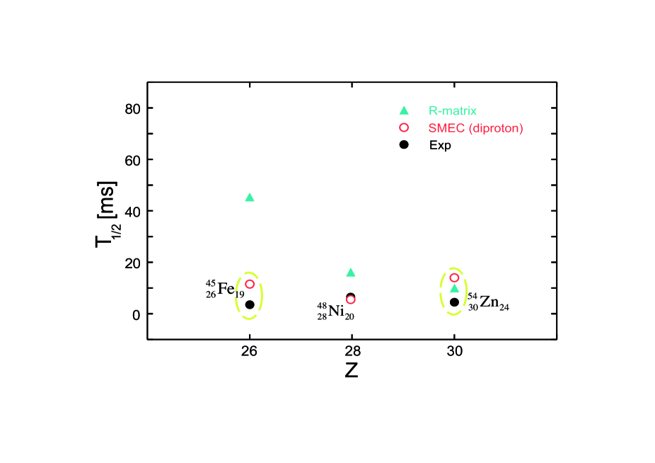
Figure 19: The partial half-lives for the diproton decay from the ground state of ${}^{45}_{26}\rm{Fe}$, ${}^{48}_{28}\rm{Ni}$, and ${}^{54}_{30}\rm{Zn}$, as calculated in the generalized R-matrix theory  [29] (full triangles) and in the SMEC [34](open circles). The experimental values are shown with black points. For reasons of clarity, the uncertainty of theoretical results due to the uncertainty of the $Q_{2p}$ values and experimental error bars are not shown.

Fig. 19 compares the experimental partial half-lives for the diproton decay of ${}^{45}_{26}\rm{Fe}$, ${}^{48}_{28}\rm{Ni}$, and ${}^{54}_{30}\rm{Zn}$ with the calculated ones in the SMEC and in the extended R-matrix model. One may notice two characteristic features from this comparison. Firstly, SMEC and R-matrix models predict a different Z-dependence of calculated 2p partial half-lives around the doubly-magic nucleus ⁴⁸Ni. Secondly, SMEC yields an opposite tendency of ⁴⁵Fe and ⁵⁴Zn half-lives with respect to the half-life of ⁴⁸Ni than seen experimentally. Concerning the first point, one may tentatively assume that this feature is related to the continuum coupling induced dynamical effects in the 2p decay which are missing in the R-matrix description. Certainly, one does not expect that this different systematic tendency of calculated half-lives in the SMEC approach and in the R-matrix model could be explained by the absence of configuration mixings beyond the 1p0f shell, since both in SMEC and in R-matrix calculations these configurations are not included. Concerning the second point, it may be related to the small number of channels in SMEC calculations of the ${\cal Q}$-${\cal P}$-coupling induced an external configuration mixing. In Ref. [34], the external mixing is a result of coupling between the ground state of nucleus $[A]$ and the two channels corresponding to the ground state and the first excited state of a nucleus $[A-1]$. This restriction on the number of channels is justified in closed-shell nuclei as in this case the ground-state to ground-state coupling of the $[A]$ and $[A-1]$ nuclei exhausts up to about 90% of the total coupling strength. For open-shell nuclei, the strength of continuum coupling is largely spread over many channels, both open and closed. Indeed, the SMEC studies of continuum coupling effects in oxygen and fluorine isotopes [159] have shown that a contribution of the ground-state to ground-state coupling to the total continuum coupling strength may vary between a few $\%$ and $\sim 30\%$ in open-shell nuclei. The size of a model space involved in the calculation of the 2p decay in ${}^{45}_{26}\rm{Fe}$, ${}^{48}_{28}\rm{Ni}$, and ${}^{54}_{30}\rm{Zn}$ makes it impossible to verify this observation numerically, but if true it may lead to a strong enhancement of the contribution from the virtual sequential 2p decay path and, henceforth, to a decrease of the 2p partial half-life. One should remind, that the interference between the virtual sequential and diproton emission paths cannot be probably neglected if both processes become equally important.

As said before, SMEC predictions are very sensitive to $Q$ values which for the nuclei studied are either not known experimentally with a sufficient precision ($Q_{2p}$ values), or are unknown ($Q_{1p}$ values). The virtual sequential decay half-lives depend explicitly and strongly on the continuum coupling dynamics between the ${\cal Q}$, ${\cal P}$ and ${\cal P}$, ${\cal T}$ subspaces which is governed by $Q$ values. A direct dependence of the diproton half-lives on ${\cal Q}$-${\cal P}$ virtual couplings is rather weak, i.e. dressing of the diproton decay mode by virtual 1p excitations does not change significantly its properties in ⁴⁵Fe, ⁴⁸Ni and ⁵⁴Zn . On the other hand, this idealized decay mode represents a sensible approximation of the 2p decay process described by (8) only if the virtual sequential decay path is strongly suppressed. This in turn depends directly on the dynamics of the ${\cal Q}$, ${\cal P}$ and ${\cal P}$, ${\cal T}$ virtual couplings. Hence, further progress in describing spontaneous 2p radioactivity and understanding the role of both pairing correlations and virtual excitations to continuum states in this process depends on a precise experimental determination of the $Q_{1p}$ and $Q_{2p}$ values.

10 Conclusions and outlook

The study of 2p emission opens a new window to investigate nucleon-nucleon correlations and the structure of atomic nuclei. Although these studies, at least partially, could have been performed already with $\beta$-delayed 2p emitters, the field received a strong boost with the observation of ground-state 2p radioactivity. This discovery triggered new experimental developments, such as time-projection chambers, and new theoretical activity related mainly to the unified description of structure and reactions with two-particle continua and the development of various methods to deal with three-body asymptotic states of charged particles/fragments.

Both experiment and theory have reached a certain level of sophistication, but significant improvements are still needed to develop 2p radioactivity into a powerful tool for nuclear structure studies. On the theoretical side, the lack of three-body asymptotic channels hampers the calculation of various correlation functions in the SMEC framework. Description of direct 2p emission with three-body asymptotics in SMEC requires inclusion of finite-range interactions. At the moment, the angular correlations between decay products can be studied solely in the three-body cluster models. The simplified description of nuclear structure in cluster models does not allow to draw deeper conclusions about 2p in-medium correlations from these angular correlations.

As one deals with three particles in the final state, the 2p emission can occur in different ways, i.e. the asymptotic channel cannot be defined unambiguously. Consequently and in contrast to one-proton or $\alpha$ radioactivity, the 2p radioactivity does not have a unique experimental signature and its interpretation is always depending on the theoretical interpretation. A complete theoretical description of 2p emission has to take into account all different decay paths and include interferences between them. It is not obvious whether different 2p decay paths, such as the diproton path and the virtual sequential 2p decay path which both yield similar proton energy distributions, can be distinguished by, e.g., the proton-proton and/or proton-fragment correlations. Further studies along this line are necessary for a best possible characterization of 2p radioactivity.

On the experimental side, more cases of 2p radioactivity have to be studied and the quality of the data has to be improved, as the possibilities to compare the experimental data existing today with modern theories of 2p radioactivity are hampered by large experimental error bars. To improve the experimental data, increased statistics is only one aspect. In the case of ⁴⁵Fe, the major contribution to the uncertainty of the decay energy comes from the energy calibration. Therefore, new and improved calibration tools have to be developed as well. A precise determination of $Q_{1p}$ and $Q_{2p}$ would help to check different features of SMEC calculations, such as the choice of effective interactions and valence space, or the absence of explicit three-body asymptotics.

All experiments performed up to now seem to indicate that the sequential decay prevails, as long as intermediate states for 1p emission are energetically accessible. The only exceptions seem to be the decays of excited states in ¹⁷Ne and in ⁹⁴Ag^m, where despite many intermediate states a strong proton-proton correlation was observed. A halo-like structure and/or dynamical effects associated with the tunnelling through the anisotropic Coulomb barrier could be at the origin of the observed correlation. Higher statistics data and advanced theoretical studies are needed to confirm or reject this interpretation.

Another application of the 2p studies are direct resonant 2p radiative capture processes [166, 167]. It was demonstrated that the astrophysical 2p capture rates can be enhanced by as much as several orders of magnitude in certain ranges of excitation energies. Similar tendency was found for the size of a nonresonant E1 contribution to the 2p capture rates [167]. These predictions may have important consequences for the rp-process path changing earlier predictions concerning rp-process waiting points [168].

The advent of new radioactive beam machines like the RIBF facility in RIKEN, Japan or the FAIR facility in GSI, Germany should give access to new ground-state 2p emitters such as ⁵⁹Ge, ⁶³Se, or ⁶⁷Kr and allow one to achieve much higher rates for the known ones. These possibilities will most likely significantly increase the body of experimental data and may establish 2p radioactivity as a powerful tool of nuclear structure studies.

These new facilities may allow also to search for a similar phenomenon which is one- and two-neutron radioactivity. From an experimental point of view, it seems to be rather difficult to find good candidates for these new decay modes. Due to the absense of the Coulomb barrier for neutrons, only the centrifugal barrier will prevent these neutrons from escaping ”immediately” from the nucleus. To create a sufficiently high barrier, high-j orbitals are needed which form the nuclear ground state only in medium-mass nuclei. However, these medium-mass neutron drip-line nuclei are rather far away from the valley of stability and extremely difficult to produce. Possibly, high-j isomers could be candidates for this kind of radioactivity.

From a theoretical point of view, two-neutron emitters would be ideal cases to study. All theoretical formalisms can be applied to the two-neutron case without major changes. Actually, the two-neutron three-body problem can be solved exactly and not approximately as in the three-body case with charged particles. Moreover, angular correlations will be directly related to the internal two-neutron correlations without the uninteresting correlations due to a possible anisotropy of the Coulomb barrier.

References

- [1] V. I. Goldansky, Nucl. Phys. 19, 482 (1960).
- [2] Y. B. Zel’dovich, Sov. Phys. JETP 11, 812 (1960).
- [3] V. A. Karnaukhov and N. I. Tarantin, Sov. Phys. JETP 12, 771 (1961).
- [4] S. Hofmann et al., Z. Phys. A305, 111 (1982).
- [5] O. Klepper et al., Z. Phys. A305, 125 (1982).
- [6] B. Blank and M. J. G. Borge, Prog. Nucl. Part. Phys. 60, 403 (2008).
- [7] K. P. Jackson et al., Phys. Lett. B33, 281 (1970).
- [8] J. Cerny, J. Esterl, R. A. Gough, and R. G. Sextro, Phys. Lett. B33, 284 (1970).
- [9] J. Cerny, R. A. Gough, R. G. Sextro, and J. Esterl, Nucl. Phys. A 188, 666 (1972).
- [10] V. I. Goldansky, Nucl. Phys. 27, 648 (1961).
- [11] V. I. Goldanskii, Nuovo Cimento 25, suppl. 2, 123 (1962).
- [12] V. I. Goldanskii, Phys. Lett. 14, 233 (1965).
- [13] V. I. Goldanskii, Sov. Phys. Uspekhi 8, 770 (1966).
- [14] J. Jänecke, Nucl. Phys. 61, 326 (1965).
- [15] B. A. Brown, Phys. Rev. C 43, R1513 (1991).
- [16] B. J. Cole, Phys. Rev. C 54, 1240 (1996).
- [17] W. E. Ormand, Phys. Rev. C 53, 214 (1996).
- [18] V. M. Galitsky and V. F. Cheltsov, Nucl. Phys. 56, 86 (1964).
- [19] J. Giovinazzo et al., Phys. Rev. Lett. 89, 102501 (2002).
- [20] M. Pfützner et al., Eur. Phys. J. A14, 279 (2002).
- [21] B. Blank et al., Phys. Rev. Lett. 94, 232501 (2005).
- [22] C. Dossat et al., Phys. Rev. C 72, 054315 (2005).
- [23] O. V. Bochkarev et al., Sov. J. Nucl. Phys. 49, 941 (1989).
- [24] R. A. Kryger et al., Phys. Rev. Lett. 74, 860 (1995).
- [25] M. D. Cable et al., Phys. Rev. Lett. 50, 404 (1983).
- [26] C. Bain et al., Phys. Lett. B373, 35 (1996).
- [27] I. Mukha et al., Nature 439, 298 (2006).
- [28] B. A. Brown, F. Barker, and D. Millener, Phys. Rev. C 65, 051309 (2002).
- [29] B. A. Brown and F. C. Barker, Phys. Rev. C 67, 041304 (2003).
- [30] K. Bennaceur, J. Dobaczewski, and M. Ploszajczak, Phys. Rev. C 60, 034308 (1999).
- [31] K. Bennaceur, F. Nowacki, J. Okołowicz, and M. Ploszajczak, Nucl. Phys. A671, 203 (2000).
- [32] J. Okołowicz, M. Płoszajczak, and I. Rotter, Phys. Rep. 374, 271 (2003).
- [33] J. Rotureau, J. Okolowicz, and M. Ploszajczak, Phys. Rev. Lett. 95, 042503 (2005).
- [34] J. Rotureau, J. Okolowicz, and M. Ploszajczak, Nucl. Phys. A767, 13 (2006).
- [35] N. Michel, W. Nazarewicz, and M. Płoszajczak, Phys. Rev. C 70, 064313 (2004).
- [36] L. Grigorenko, I. Mukha, and M. Zhukov, Nucl. Phys. A713, 372 (2003).
- [37] C. Kurokawa and K. Kato, Nucl. Phys. A738, 455 (2004).
- [38] E. Garrido, D. V. Fedorov, and A. S. Jensen, Nucl. Phys. A733, 85 (2004).
- [39] V. I. Goldanskii, Ann. Rev. Nucl. Sci 16, 1 (1966).
- [40] J. Äystö and J. Cerny, Treatise on Heavy Ion Science, Vol. 8, D.A. Bromley, Ed. 207 (1989).
- [41] R. Barton et al., Can. J. Phys. 41, 2007 (1963).
- [42] P. J. Woods and C. N. Davids, Annu. Rev. Nucl. Part. Sci. 47, 541 (1997).
- [43] K. Rykaczewski, Eur. Phys. J. A 15, 81 (2002).
- [44] D. Seweryniak et al., Phys. Rev. Lett. 86, 1458 (2001).
- [45] V. A. Karnaukhov and Lu Hsi-Ting, Sov. Phys. JETP 20, 860 (1965).
- [46] J. Jänecke, Preprint K.F.K. 185 (Kernforschungszentrum, Karlsruhe) (1963).
- [47] G. Audi, O. Bersillon, J. Blachot, and A. H. Wapstra, Nucl. Phys. A729, 3 (2003).
- [48] G. Charpak et al., Phys. Lett. 16, 54 (1965).
- [49] R. L. Burman and M. E. Nordberg, Phys. Lett. 21, 229 (1968).
- [50] F. Ajzenberg-Selove, C. F. Osgood, and C. P. Baker, Phys. Rev. 116, 1521 (1959).
- [51] D. F. Geesaman et al., Phys. Rev. C 15, 1835 (1977).
- [52] O. V. Bochkarev et al., Sov. J. Nucl. Phys. 55, 955 (1992).
- [53] A. Azhari, R. Kryger, and M. Thoennessen, Phys. Rev. C 58, 2568 (1998).
- [54] A. M. Lane and R. G. Thomas, Rev. Mod. Phys. 30, 257 (1958).
- [55] L. Axelsson et al., Phys. Rev. C 54, R1511 (1996).
- [56] A. Lépine-Szily et al., Phys. Rev. Lett. 80, 1601 (1998).
- [57] A. Azhari et al., Phys. Rev. C 57, 628 (1998).
- [58] I. Mukha, (private communication).
- [59] P. Masson and J. Jänecke, At. Data Nucl. Data Tab. 39, 273 (1988).
- [60] M. S. Antony, A. Pape, and J. Britz, At. Data Nucl. Data Tab. 66, 1 (1997).
- [61] C. Woodward, R. Tribble, and D. Tanner, Phys. Rev. C 27, 27 (1983).
- [62] V. I. Goldanskii, Sov. Phys. JETP Lett. 32, 554 (1980).
- [63] M. D. Cable et al., Phys. Rev. C 26, 1778 (1982).
- [64] R. Jahn et al., Phys. Rev. C 31, 1576 (1985).
- [65] J. Honkanen et al., Phys. Lett. B133, 146 (1983).
- [66] J. Äystö et al., Phys. Rev. Lett. 55, 1384 (1985).
- [67] B. Blank et al., Z. Phys. A 357, 247 (1997).
- [68] V. Borrel et al., Nucl. Phys. A473, 331 (1987).
- [69] J. E. Reiff et al., Nucl. Instrum. and Meth. A276, 228 (1989).
- [70] D. M. Moltz et al., Z. Phys. A 342, 273 (1992).
- [71] V. Borrel et al., Z. Phys. A 344, 135 (1992).
- [72] J. Giovinazzo et al., Phys. Rev. Lett. 99, 102501 (2007).
- [73] C. Dossat et al., Nucl. Phys. A 792, 18 (2007).
- [74] L. Axelsson et al., Nucl. Phys. A628, 345 (1998).
- [75] L. Axelsson et al., Nucl. Phys. A634, 475 (1998).
- [76] J. Thaysen et al., Phys. Lett. B467, 194 (1999).
- [77] H. Fynbo et al., Phys. Rev. C 59, 2275 (1999).
- [78] B. A. Brown, Phys. Rev. Lett. 65, 2753 (1991).
- [79] N. Adimi, (private communication).
- [80] M. B. Greenfield, C. R. Bingham, E. Newman, and M. J. Saltmarsh, Phys. Rev. C 6, 1756 (1972).
- [81] M. Chromik et al., Phys. Rev. C 55, 1676 (1997).
- [82] M. Chromik et al., Phys. Rev. C 66, 024313 (2002).
- [83] T. Zerguerras et al., Eur. Phys. J. A20, 389 (2004).
- [84] Y. Blumenfeld et al., Nucl. Instr. Meth. A421, 471 (1999).
- [85] L. Bianchi et al., Nucl. Instr. Meth. A276, 509 (1989).
- [86] R. Kanungo et al., Phys. Lett. B571, 21 (2003).
- [87] L. V. Grigorenko, Y. L. Parfenova, and M. V. Zhukov, Phys. Rev. C 71, 051604R (2005).
- [88] A. Le Fèvre et al., Nucl. Phys. A 735, 219 (2004).
- [89] J. Gomez del Campo et al., Phys. Rev. Lett. 86, 43 (2001).
- [90] M. L. Commara et al., Nucl. Phys. A 708, 167 (2002).
- [91] C. Plettner et al., Nucl. Phys. A 733, 20 (2004).
- [92] I. Mukha et al., Phys. Rev. C 70, 044311 (2004).
- [93] I. Mukha et al., Phys. Rev. Lett. 95, 022501 (2005).
- [94] E. Roeckl, Int. J. Mod. Phys. E 15, 368 (2006).
- [95] V. I. Goldanskii, Phys. Lett. B212, 11 (1988).
- [96] C. Détraz et al., Nucl. Phys. A519, 529 (1990).
- [97] L. Faux et al., Phys. Rev. C 49, 2440 (1994).
- [98] B. Blank et al., Nucl. Instrum. Meth. A330, 83 (1993).
- [99] B. Blank et al., Phys. Rev. Lett. 77, 2893 (1996).
- [100] B. Blank et al., Phys. Rev. Lett. 84, 1116 (2000).
- [101] A. C. Mueller and R. Anne, Nucl. Instrum. Meth. B56, 559 (1991).
- [102] J. Giovinazzo et al., Eur. Phys. J. A10, 73 (2001).
- [103] W. E. Ormand, Phys. Rev. C 55, 2407 (1997).
- [104] B. A. Brown et al., Phys. Rev. C 65, 045802 (2002).
- [105] J. Giovinazzo et al., Eur. Phys. J. A11, 247 (2001).
- [106] B. Blank et al., to be published (2007).
- [107] K. Miernik et al., Nucl. Instrum. Methods Phys. Res., Sect. A 581, 194 (2007).
- [108] F. Sauli, Nucl. Instr. Meth. A 386, 531 (1997).
- [109] R. Bellazzini et al., Nucl. Instrum. Meth. A424, 444 (1999).
- [110] K. Miernik et al., Phys. Rev. Lett. 99, 192501 (2007).
- [111] L. Grigorenko et al., Phys. Rev. C 64, 054002 (2001).
- [112] J. Dobaczewski and W. Nazarewicz, Philos. Trans. R. Soc. London, Ser. A 356, 2007 (1998).
- [113] J. Dobaczewski et al., Prog. Part. Nucl. Phys. in print (2007).
- [114] A. Baz’, Y. B. Zel’dovich, and A. Perelomov, Scattering, Reactions and Decay in Nonrelativistic Quantum Mechanics Israel Program for Scientific Translations Ltd., IPST Cat. No. 5149 (1969).
- [115] H. Feshbach, Ann. Phys. 5, 357 (1958).
- [116] H. Feshbach, Ann. Phys. 19, 287 (1962).
- [117] U. Fano, Phys. Rev. 124, 1866 (1961).
- [118] C. Mahaux and H. Wiedenmüller, Shell Model Approach to Nuclear Reactions, North-Holland, Amsterdam (1969).
- [119] R. J. Philpott, Nucl. Phys. A289, 109 (1977).
- [120] D. Halderson and R. J. Philpott, Nucl. Phys. A345, 141 (1980).
- [121] H. W. Barz, I. Rotter, and J. Höhn, Nucl. Phys. A275, 111 (1977).
- [122] H. W. Barz, I. Rotter, and J. Höhn, Nucl. Phys. A307, 285 (1978).
- [123] I. Rotter, Rep. Prog. Phys. 54, 635 (1991).
- [124] A. Volya and V. Zelevinsky, Phys. Rev. C 67, 054322 (2003).
- [125] A. Volya and C. Davids, Eur. Phys. J. A 25, 161 (2005).
- [126] D. V. Fedorov, A. S. Jensen, and K. Riisager, Phys. Rev. C 50, 2372 (1994).
- [127] E. Nielsen, D. V. Fedorov, A. S. Jensen, and E. Garrido, Phys. Rep. 347, 373 (2001).
- [128] L. Grigorenko and M. Zhukov, Phys. Rev. C 68, 054005 (2003).
- [129] L. Grigorenko, I. Mukha, and M. Zhukov, Nucl. Phys. A714, 425 (2003).
- [130] N. Michel, W. Nazarewicz, M. Płoszajczak, and J. Okołowicz, Phys. Rev. Lett. 89, 042502 (2002).
- [131] R. I. Betan, R. J. Liotta, N. Sandulescu, and T. Vertse, Phys. Rev. Lett. 89, 042501 (2002).
- [132] J. B. Faes, PhD thesis, University of Caen (2007).
- [133] W. Wang and C. Shakin, Pyhs. Lett. B 32, 421 (1970).
- [134] E. Garrido, D. V. Fedorov, A. S. Jensen, and H. O. U. Fynbo, Nucl. Phys. A748, 39 (2005).
- [135] K. M. Watson, Phys. Rev. 88, 1163 (1952).
- [136] A. B. Migdal, Sov. Phys. JETP 28, 3 (1955).
- [137] F. C. Barker, Phys. Rev. C 63, 047303 (2001).
- [138] R. Chatterjee, J. Okolowicz, and M. Ploszajczak, Nucl. Phys. A764, 528 (2006).
- [139] N. Michel, W. Nazarewicz, and M. Płoszajczak, Phys. Rev. C 75, (R)031301 (2007).
- [140] N. Michel, W. Nazarewicz, and M. Płoszajczak, Nucl. Phys. A794, 29 (2007).
- [141] K. Ikeda, N. Takigawa, and H. Horiuchi, Prog. Theor. Phys. Suppl. Extra Number 464 (1968).
- [142] P. Y. Luo, J. Okołowicz, M. Płoszajczak, and N. Michel, arXiv:nucl-th/0201073 .
- [143] N. Michel, W. Nazarewicz, F. Nowacki, and M. Płoszajczak, Nucl. Phys. A752, 335c (2005).
- [144] J. Okołowicz and M. Płoszajczak, Int. J. Mod. Phys. E 15, 529 (2006).
- [145] W. Glöckle et al., Phys. Rep. 274, 107 (1996).
- [146] G. Tanner, K. Richter, and J. M. Rost, Rev. Mod. Phys. 72, 497 (2000).
- [147] C. D. Lin, Phys. Rep. 257, 1 (1995).
- [148] T. N. Rescigno, M. Baertschy, W. A. Isaacs, and C. W. McCurdy, Science 286, 2464 (1999).
- [149] E. Alt, S. Levin, and S. Yakovlev, Phys. Rev. C 69, 034002 (2004).
- [150] A. Deltuva, A.C. Fonseca, and P.U. Sauer, Phys. Rev. C 71, 054005 (2005); ibid. C 72, 054004 (2005); C 73, 057001 (2006).
- [151] L.V. Grigorenko, R.C. Johnson, I.G. Mukha, I.J. Thompson, and M.V. Zhukov, Phys. Rev. C 64, 054002 (2001).
- [152] L.V. Grigorenko, R.C. Johnson, I.G. Mukha, I.J. Thompson, and M.V. Zhukov, Phys. Rev. Lett. 85, 22 (2000).
- [153] E. Garrido, D. V. Fedorov, A. S. Jensen, and H. O. U. Fynbo, Nucl. Phys. A748, 27 (2005).
- [154] E. Garrido, D. V. Fedorov, A. S. Jensen, and H. O. U. Fynbo, Nucl. Phys. A766, 74 (2006).
- [155] E. Garrido, D. V. Fedorov, and A. S. Jensen, Nucl. Phys. A617, 153 (1997).
- [156] M. V. Zhukov et al., Phys. Rep. 231, 151 (1993).
- [157] L. V. Grigorenko et al., Phys. Rev. C 57, R2099 (1998).
- [158] L. V. Grigorenko et al., Phys. Rev. C 60, 044312 (1999).
- [159] J. Okołowicz, and M. Płoszajczak, and Y. Luo, Proc. XXX Mazurian Lakes Conference on Physics: Nuclear Physics and Fundamental Processes, Acta Physica Polonica (2008), in print.
- [160] S. Nummela et al., Phys. Rev. C 63, 044316 (2001).
- [161] M. Honma, T. Otsuka, B. A. Brown, and T. Mizusaki, Phys. Rev. C 65, 061301 (2002).
- [162] M. Honma, T. Otsuka, B. A. Brown, and T. Mizusaki, Phys. Rev. C 69, 034335 (2004).
- [163] W. A. Richter, M. G. V. D. Merwe, R. E. Julies, and B. A. Brown, Nucl. Phys. A523, 325 (1991).
- [164] A. Poves and A. P. Zuker, Phys. Rep. 70, 235 (1981).
- [165] P. Decowski, W. Benenson, B. A. Brown, and H. Nann, Nucl. Phys. A302, 186 (1978).
- [166] L. V. Grigorenko and M. V. Zhukov, Phys. Rev. C 72, 015803 (2005).
- [167] L. V. Grigorenko, K. Langanke, N. B. Shul’gina, and M. V. Zhukov, Phys. Lett. B641, 254 (2006).
- [168] J. Görres, M. Wiescher, and F.-K. Thielemann, Phys. Rev. C 51, 392 (1995).