Little Higgs Model Discrimination at the LHC and ILC

Abstract

We propose a means to discriminate between the two basic variants of Little Higgs models, the Product Group and Simple Group models, at the next generation of colliders. It relies on a special coupling of light pseudoscalar particles present in Little Higgs models, the pseudoaxions, to the $Z$ and the Higgs boson, which is present only in Simple Group models. We discuss the collider phenomenology of the pseudoaxion in the presence of such a coupling at the LHC, where resonant production and decay of either the Higgs or the pseudoaxion induced by that coupling can be observed for much of parameter space. The full allowed range of parameters, including regions where the observability is limited at the LHC, is covered by a future ILC, where double scalar production would be a golden channel to look for.

1 Pseudoaxions in Little Higgs Models

Little Higgs Models lhm_moose provide a solution to the hierarchy problem, as they stabilize the Higgs boson against quadratic divergences at the one-loop level by the mechanism of collective symmetry breaking: the Higgs is charged under two global symmetry groups, which both need to be broken in order to lift the flat direction in the potential of the Higgs boson and make it a pseudo-Nambu-Goldstone boson (PNGB). Collective breaking models can be classified in three different categories, the so-called moose models with a moose diagram structure of links of global and local symmetry groups, the product-group models and the simple-group models. In the product-group models (the most-studied case is the Littlest Higgs) the electroweak gauge group is doubled, broken down to the group $SU(2)_{L}$, while the Higgs shares together with the other PNGBs an irreducible representation of the coset space of the symmetry breaking. On the other hand, in simple-group models the electroweak gauge group is enlarged to a simple $SU(N)$ group, while the Higgs is distributed over several multiplets of the global symmetry group, which usually has a product group structure similar to chiral symmetries in QCD simple . For an overview see review .

Figure 1: Branching ratios of the pseudoaxion $\eta$ in the Simplest Little Higgs as a function of its mass.

The two crucial scales in the Little Higgs set-up are the cut-off scale $\Lambda$ where the models are embedded in a UV-complete theory (usually a strongly-interacting theory with a partonic substructure of the PNGBs) and the intermediate scale $F$ which determines the masses and decay constants of the PNGBs (except for the Higgs which is down at $v$ by the collective symmetry breaking mechanism). Electroweak precision observables and direct search limits lowenergy tell us that the scale $F$ must be at least of the order of $1-2$ TeV. Paradoxically, the Higgs boson in Little Higgs models tends to be quite heavy compared to the Standard Model or the MSSM, of the order of $200-600$ GeV little_kr . For Little Higgs model scales that high most new particles will be produced close to the kinematical limit at the LHC, such that a precision determination of their parameters might be difficult. Furthermore, also the sensitivity of the ILC in indirect measurements might be limited, if the new physics does couple to SM fermions only very weakly resonances . A method to distinguish between different models, especially at the LHC, is highly welcome. Such a method will be presented here.

Little Higgs models generally have a huge global symmetry group, which contains not only products of simple groups but also a certain number of $U(1)$ factors. These Abelian groups can either be gauged, in which case they lead to a $Z^{\prime}$ boson, or they are only (approximate) global symmetries. In the latter case there is a PNGB attached to that spontaneously broken global $U(1)$ factor pseudoaxions . The number of pseudoaxions in a given model is determined by the mismatch between the rank reduction in the global and the local symmetry group, since it gives the number of uneaten bosons. In the Littlest Higgs, e.g., there is one such pseudoaxion, in the Simplest Little Higgs simplest there is one, in the original simple group model there are two, in the minimal moose model there are four, and so on.

These particles are electroweak singlets, hence all couplings to SM particles are suppressed by the ratio of the electroweak over the Little Higgs scale, $v/F$. There mass lies in the range from several GeV to a few hundred GeV, being limited by a naturalness argument and the stability of the Coleman-Weinberg potential. For the Simplest Little Higgs, on whose phenomenology we will concentrate here, there is a seesaw between the Higgs and the pseudoscalar mass pseudoaxions , determined by the explicit symmetry breaking parameter $\mu$, where $m_{\eta}\approx\sqrt{2}\mu$. Since the pseudoaxions $\eta$ inherit the Yukawa coupling structure from the Higgs bosons, they decay predominantly to the heaviest available fermions in the SM, and because of the absence of the $WW$ and $ZZ$ modes, the anomaly-induced decays $gg$ and $\gamma\gamma$ are sizable over a wide mass range, cf. Fig. 1. From this, one can see that as soon as the decay to $HZ$ is kinematically allowed, it dominates completely. Such a $\eta HZ$ coupling, which is possible only after electroweak symmetry breaking and hence proportional to $v/F$, is only allowed in simple group models and is forbidden to all orders in product group models. One can factor out the $U(1)_{\eta}$ group from the matrix of PNGBs. We use $\xi=\exp\left[i\eta/F\right]$ for the pseudoaxion field and $\Sigma=\exp\left[i\Pi/F\right]$ for the non-linear representation of the remaining Goldstone multiplet $\Pi$ of Higgs and other heavy scalars. Then, for product group models, the kinetic term may be expanded as

$$\mathcal{L}_{\text{kin.}} \sim\;F^{2}\text{Tr}\left[(D^{\mu}(\xi\Sigma)^{\dagger}(D_{\mu}(\xi\Sigma))\right]$$

$$=\;\ldots-2F(\partial_{\mu}\eta)\,\text{Im}\text{Tr}\left[(D^{\mu}\Sigma)^{\dagger}\Sigma\right]+O(\eta^{2}),$$ (1)

where we write only the term with one derivative acting on $\xi$ and one derivative acting on $\Sigma$. This term, if nonzero, is the only one that can yield a $ZH\eta$ coupling.

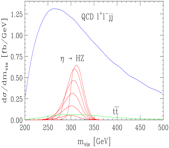
Figure 2: Case: heavy $\eta$, light Higgs, invariant mass for the $\ell\ell bb$ final state for $\eta\to HZ$, $Z\to\ell\ell$ and $\eta\to bb$. The QCD background is blue, the top background green. The pseudoaxion signal is red for a mass varying from 280 to 335 GeV.

We now use the special structure of the covariant derivatives in product group models, which is the key to the Little Higgs mechanism: $D_{\mu}\Sigma=\partial_{\mu}\Sigma+A_{1,\mu}^{a}\left(T_{1}^{a}\Sigma+\Sigma(T_{1}^{a})^{T}\right)+A_{2,\mu}^{a}\left(T_{2}^{a}\Sigma+\Sigma(T_{2}^{a})^{T}\right)$, where $T_{i}^{a},i=1,2$ are the generators of the two independent $SU(2)$ groups, and $A_{i,\mu}^{a}=W^{a}_{\mu}$ + heavy fields. Neglecting the heavy gauge fields and extracting the electroweak gauge bosons, we have $\text{Tr}\left[(D^{\mu}\Sigma)^{\dagger}\Sigma\right]\sim W_{\mu}^{a}\text{Tr}\left[(T_{1}^{a}+T_{2}^{a})+(T_{1}^{a}+T_{2}^{a})^{*}\right]=0$. This vanishes due to the zero trace of $SU(2)$ generators. The same is true when we include additional $U(1)$ gauge group generators such as hypercharge, since their embedding in the global simple group forces them to be traceless as well. We conclude that the coefficient of the $ZH\eta$ coupling vanishes to all orders in the $1/F$ expansion.

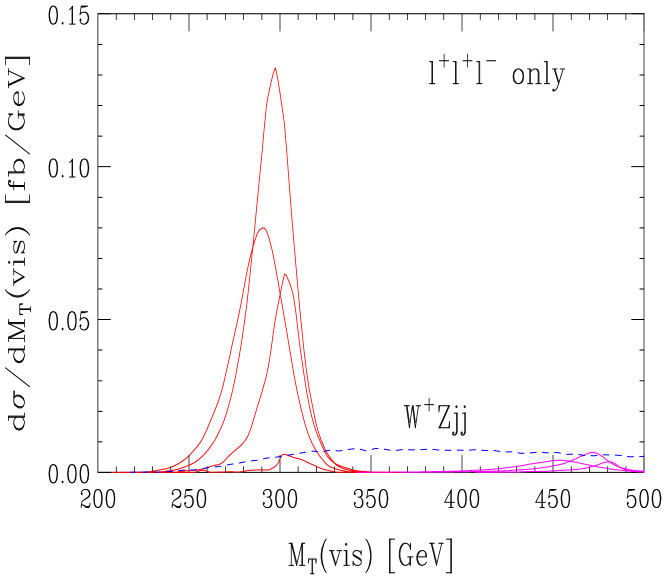
Figure 3: Case: heavy $\eta$, heavy Higgs, process: $gg\to\eta\to ZH$, $Z\to\ell\ell$, $\eta\to WW$; invariant visible mass distribution for $\ell\ell\ell jj/\!\!\!p_{T}$. There is only a tiny background from $WZjj$ (dashed line).

Next, we consider the simple group models, where we use the following notation for the nonlinear sigma fields: $\Phi\zeta$, where $\Phi=\exp[i\Sigma/F]$ and $\zeta=\left(0,\ldots 0,F\right)^{T}$ is the vev directing in the $N$ direction for an $SU(N)$ simple gauge group extension of the weak group. Thus, in simple group models the result is the $N,N$ component of a matrix:

$$\mathcal{L}_{\text{kin.}} \sim\;F^{2}D^{\mu}(\zeta^{\dagger}\Phi^{\dagger})D_{\mu}(\Phi\zeta)$$

$$=\;\ldots+iF(\partial_{\mu}\eta)\left(\Phi^{\dagger}(D_{\mu}\Phi)-(D_{\mu}\Phi^{\dagger})\Phi\right)_{N,N}\;.$$ (2)

We separate the last row and column in the matrix representations of the Goldstone fields $\Sigma$ and gauge boson fields $\mathbf{V}_{\mu}$: the Higgs boson in simple group models sits in the off-diagonal entries of $\Sigma$, while the electroweak gauge bosons reside in the upper left corner of $\mathbf{V}_{\mu}$. With the Baker-Campbell-Hausdorff identity, one gets for the term in parentheses in Eq. (1):

$$\;\mathbf{V}_{\mu}+\frac{i}{F}[\Sigma,\mathbf{V}_{\mu}]-\frac{1}{2F^{2}}[\Sigma,[\Sigma,\mathbf{V}_{\mu}]]+\ldots$$

$$= \;\begin{pmatrix}\mathbf{W}_{\mu}&0\\ 0&0\end{pmatrix}+\frac{i}{F}\begin{pmatrix}0&-\mathbf{W}_{\mu}h\\ h^{\dagger}\mathbf{W}_{\mu}&0\end{pmatrix}$$ (3)

$$\;-\frac{1}{2F^{2}}\begin{pmatrix}hh^{\dagger}\mathbf{W}+\mathbf{W}hh^{\dagger}&0\\ 0&-2h^{\dagger}\mathbf{W}h\end{pmatrix}+\ldots$$

The $N,N$ entry can only be nonzero from the third term on. The first term, would be a mixing between the $\eta$ and the Goldstone boson(s) for the $Z^{\prime}$ state(s) and cancels with the help of the many-multiplet structure. If the $N,N$ component of the second term were nonzero, it would induce a $ZH\eta$ coupling without insertion of a factor $v$. This is forbidden by electroweak symmetry. To see this, it is important to note that in simple group models the embedding of the Standard Model gauge group always works in such a way that hypercharge is a linear combination of the $T_{N^{2}-1}$ and $U(1)$ generators. This has the effect of canceling the $\gamma$ and $Z$ from the diagonal elements beyond the first two positions, and preventing the diagonal part of $\mathbf{W}_{\mu}$ from being proportional to $\tau^{3}$. The third term in the expansion yields a contribution to the $ZH\eta$ coupling, $(\partial^{\mu}\eta)h^{\dagger}\mathbf{W}_{\mu}h\sim vHZ_{\mu}\partial^{\mu}\eta$.

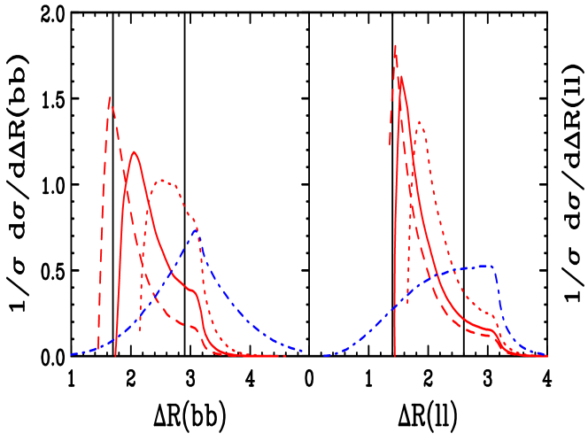
Figure 4: Lego plot separations for $b$–$b$ and $\ell$–$\ell$ for the $bb\ell\ell$ final state. The signal is red (with $m_{\eta}$ varying from around 300 to 330 GeV) and the QCD background is blue.

The crucial observation is that the matrix representation embedding of the two non-Abelian $SU(2)$ gauge groups, and especially of the two $U(1)$ factors within the irreducible multiplet of the PNGBs of one simple group (e.g. $SU(5)$ in the Littlest Higgs), is responsible for the non-existence of this coupling in product group models. It is exactly the mechanism which cancels the quadratic one-loop divergences between the electroweak and heavy $SU(2)$ gauge bosons which cancels this coupling. In simple group models the Higgs mass term cancellation is taken over by enlarging $SU(2)$ to $SU(N)$, and the enlarged non-Abelian rank structure cancels the quadratic divergences in the gauge sector – but no longer forbids the $ZH\eta$ coupling. Hence, its serves as a discriminator between the classes of models.

2 LHC and ILC phenomenology

The pseudoaxion(s) can be produced at the LHC in gluon fusion and discovered in the rare decay mode $\gamma\gamma$ pseudoaxions . But the $\eta HZ$ coupling can be observed at the LHC only if either one of the decays $H\to Z\eta$ or $\eta\to ZH$ is kinematically allowed. This leaves large holes in parameter space, which can be covered by a $500-1000$ GeV ILC, depending on the masses (see below). Here, we focus on the discovery potential of the LHC for the pseudoaxions, assuming the presence of the $ZH\eta$ coupling. We assume the Simplest Little Higgs with parameters chosen to fulfill the low-energy constraints. The two cases a) $gg\to\eta\to HZ$ and b) $gg\to H\to\eta Z$ lead to similar final states, depending on the masses of the Higgs and pseudoaxion. For light Higgs or light pseudoaxion, a) and b) lead to the final state $bb\ell\ell$, while case a) for heavier Higgs leads to a $ZWW\to\ell\ell\ell jj/\!\!\!p_{T}$ final state. In the first case, there is severe background from continuum QCD $\ell\ell jj$ production, while the top background is manageable. We apply the following cuts: $p_{T}(b)>25~{}{\rm GeV}$, $|\eta(b)|<2.5$, $p_{T}(\ell)>15~{}{\rm GeV}$, $|\eta(\ell)|<2.5$, $\triangle R(bb,b\ell)>0.4$, $\triangle R(\ell\ell)>0.2$; furthermore $89.6<m_{\ell\ell}<92.8~{}{\rm GeV}$ and   $/\!\!\!p_{T}<30~{}{\rm GeV}$ to reduce the top background. The result for the total transverse invariant mass is shown in Fig. 2, where the Simplest Little Higgs is shown for the Golden Point simplest ; pseudoaxions . Fig. 3 shows the total visible invariant mass for the final state $\ell\ell\ell jj/\!\!\!p_{T}$ which covers the case of a heavy pseudoaxion decaying to a leptonically decaying $Z$ and a heavy Higgs. The latter decays to $WW$ with one hadronic and one leptonic decay. For this process, the main background comes from $WZjj$ which is not severe for the Golden Point of the Simplest Little Higgs.

Relaxing the parameter values for the Golden Point (which gives near-to-maximal rates but is still consistent with electroweak precision observables simplest ; pseudoaxions ) reduces the signal to the size of the background. Compared to other new physics scenarios this is still a quite comfortable situation. Fig. 4 shows the method of lego plots as a further means to discriminate between signal and background. On the left, there is the $\Delta R$ for the two $b$ jets, on the right for the two leptons. The shapes of these distributions are different between signal and background and allow for a further optimization of the cut analysis to improve the signal-to-background ratio. However, this goes beyond the scope of this study here.

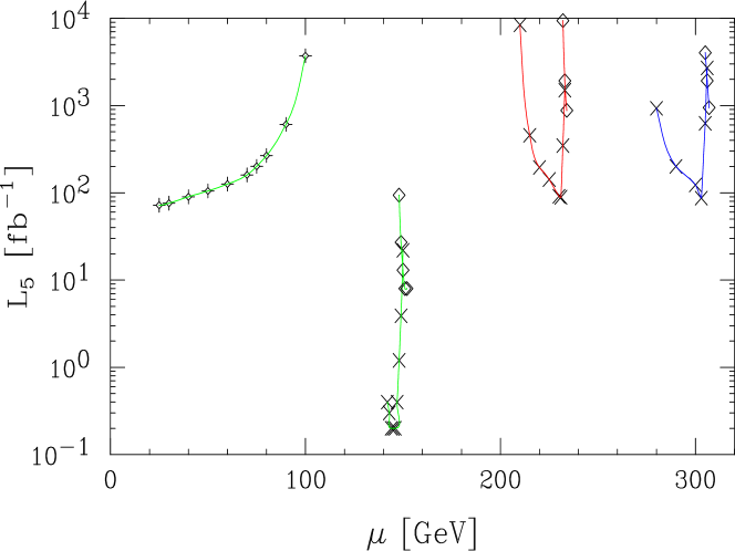
Figure 5: Needed total integrated luminosity for the LHC to yield a $5\,\sigma$ $\eta$ discovery signal. Hatches are for $gg\to\eta\to HZ$, crosses for $gg\to H\to\eta Z$. Different colors are for different choices of parameters in the Simplest Little Higgs.

Finally, Fig. 5 shows the LHC integrated luminosity (per experiment) needed for a 5 $\sigma$ discovery of the pseudoaxion in Simplest Little Higgs Model using the $\eta HZ$ coupling (for other discovery methods, cf. pseudoaxions ). Hatches in the plot are for $gg\to\eta\to HZ$, crosses for $gg\to H\to\eta Z$. Different colors are for different choices of parameters in the Simplest Little Higgs; for more details see distinguish . Remember, that this only holds if either of the two decays $\eta\to HZ$ or $H\to\eta Z$ is on-shell.

At a high-energy ILC, the production happens in association with a Higgs boson like in a two-Higgs-model. Fig. 6 shows the cross section as a function of $\sqrt{s}$ for three different values of the $\eta$ mass. The simulations for these processes have been performed with the WHIZARD package omega ; whizard ; omwhiz , which is ideally suited for physics beyond the SM omwhiz_bsm . SM backgrounds are nowhere an issue. Interesting is the $ZHH$ final state which is important for measuring the triple Higgs coupling triplehiggs . In the SM the cross section is at the borderline of detectability, but the rates are larger by factors two to six in the Simplest Little Higgs with the intermediate pseudoaxion. For more details see distinguish ; jr_lcws07 .

Figure 6: ILC cross section for the $H\eta$ associated production as function of $\sqrt{s}$, taking into account the destructive $Z/Z^{\prime}$ interference. The full, dashed and dotted lines correspond to $m_{\eta}=309/200/50$ GeV, respectively.

In conclusion, the LHC provides an ideal environment for discovering pseudoaxions and measuring their properties. The $ZH\eta$ coupling can be used as a tool for the discrimination between simple and product group models. Holes in parameter space left over by LHC can be closed by a 1 TeV ILC.

3 Acknowledgments

JR was partially supported by the Helmholtz-Gemeinschaft under Grant No. VH-NG-005 and the Bundesministerium für Bildung und Forschung, Germany, under Grant No. 05HA6VFB.

References

- (1) N. Arkani-Hamed et al., JHEP 0208 (2002) 021; N. Arkani-Hamed, A. G. Cohen, H. Georgi, Phys. Lett. B 513 (2001) 232; N. Arkani-Hamed, A. G. Cohen, T. Gregoire, and J. G. Wacker, JHEP 0208 (2002) 020; N. Arkani-Hamed, A. G. Cohen, E. Katz, and A. E. Nelson, JHEP 0207 (2002) 034.
- (2) D. E. Kaplan and M. Schmaltz, JHEP 0310 (2003) 039.
- (3) M. Schmaltz and D. Tucker-Smith, Ann. Rev. Nucl. Part. Sci. 55, 229 (2005); M. Perelstein, Prog. Part. Nucl. Phys. 58, 247 (2007); S. Heinemeyer et al., hep-ph/0511332; S. Kraml et al., CPNSH report.
- (4) C. Csáki et al., Phys. Rev. D 67 (2003) 115002; Phys. Rev. D 68 (2003) 035009; J. L. Hewett, F. J. Petriello, and T. G. Rizzo, JHEP 0310 (2003) 062; M.-C. Chen and S. Dawson, Phys. Rev. D 70 (2004) 015003. T. Han, H. E. Logan, B. McElrath, and L.-T. Wang, Phys. Rev. D 67 (2003) 095004; G. Burdman, M. Perelstein, and A. Pierce, Phys. Rev. Lett. 90 (2003) 241802 M. Perelstein, M. E. Peskin, and A. Pierce, Phys. Rev. D 69 (2004) 075002; T. Han, H. E. Logan and L. T. Wang, JHEP 0601, 099 (2006); A. J. Buras et al. JHEP 0611,062 (2006); G. Azuelos et al., Eur. Phys. J. C 39S2, 13 (2005); B. C. Allanach et al., hep-ph/0602198; K. Cheung et al., hep-ph/0608259; J. Boersma, Phys. Rev. D74, 115008 (2006).
- (5) M. Beyer et al., Eur. Phys. J. C 48, 353 (2006); W. Kilian and J. Reuter, hep-ph/0507099; J. Reuter, arXiv:0708.4383 [hep-ph].
- (6) W. Kilian and J. Reuter, Phys. Rev. D 70 (2004) 015004.
- (7) W. Kilian, D. Rainwater and J. Reuter, Phys. Rev. D 71, 015008 (2005); hep-ph/0507081.
- (8) M. Schmaltz, JHEP 0408 (2004) 056.
- (9) W. Kilian, D. Rainwater and J. Reuter, Phys. Rev. D 74, 095003 (2006).
- (10) T. Ohl, O’Mega: An Optimizing Matrix Element Generator, hep-ph/0011243; M. Moretti, T. Ohl, J. Reuter, hep-ph/0102195; J. Reuter, arXiv:hep-th/0212154.
- (11) W. Kilian. WHIZARD, 2nd ECFA/DESY Study 1998-2001, 1924-1980, LC-TOOL-2001-039, Jan 2001.
- (12) http://whizard.event-generator.org; W. Kilian, T. Ohl, J. Reuter, to appear in Comput. Phys. Commun., arXiv:0708.4233 [hep-ph].
- (13) T. Ohl and J. Reuter, Eur. Phys. J. C 30, 525 (2003); Phys. Rev. D 70, 076007 (2004); K. Hagiwara et al., Phys. Rev. D 73, 055005 (2006); J. Reuter et al., arXiv:hep-ph/0512012; W. Kilian, J. Reuter and T. Robens, Eur. Phys. J. C 48, 389 (2006); J. Reuter, arXiv:0709.0068 [hep-ph].
- (14) A. Djouadi, W. Kilian, M. Mühlleitner and P. M. Zerwas, Eur. Phys. J. C 10, 27 (1999).
- (15) J. Reuter, arXiv:0708.4241 [hep-ph].