Flavors in an expanding plasma

Abstract

We consider the effect of an expanding plasma on probe matter by determining time-dependent D7 embeddings in the holographic dual of an expanding viscous plasma. We calculate the chiral condensate and meson spectra including contributions of viscosity. The chiral condensate essentially confirms the expectation from the static black hole. For the meson spectra we propose a scheme that is in agreement with the adiabatic approximation. New contributions arise for the vector mesons at the order of the viscosity terms.

I Introduction

The study of the properties of strongly interacting quark-gluon plasma (QGP) review is one of the most investigated research topics in recent years. The interest is fueled on the one hand by direct experimental questions related to the properties of QGP produced at RHIC and on the other hand by the possibility of studying analytically the non-perturbative properties of plasmas in various, mostly supersymmetric, gauge theories using the AdS/CFT correspondence adscft . Although there does not exist so far a direct counterpart of the QCD plasma, the study of exact properties of similar systems not based on ad-hoc phenomenological models may increase our understanding of the properties of the QCD plasma. This hope has been substantiated, e.g., by the discovery of a universal strong coupling shear viscosity to entropy ratio, which is valid for a wide range of different gauge theories son ; other .

A lot of work has been initially undertaken for a static plasma system with a fixed constant temperature. After the earliest investigations of transport coefficients various other observables have been discussed related to the properties of fundamental flavors in the thermal medium such as drag force calculations Gubser:2006bz ; Herzog:2006gh , jet-quenching Liu:2006ug ; Bertoldi:2007sf ; Cotrone:2007qa , meson spectrum KMMW ; ErdmengerEvans , meson melting Hoyos:2006gb , thermodynamics of fundamental flavors Mateos:2007vn .

On the other hand, since the experimentally produced plasma is always a non-static expanding system, it was tempting to extend the AdS/CFT investigations to such a time-dependent dynamical setting. Qualitative duals for thermalization and cooling have been suggested in nastase ; zahed , a quantitative framework for studying boost-invariant expansion of a plasma system in $\mathcal{N}=4$ SYM has been proposed in JP1 . Subsequent work within this framework include SJSIN ; Heller:2007qt ; RJ ; JP2 ; BAK ; SJSIN2 ; Kajantie ; Siopsis ; Kovchegov , which concentrated on the details of the dynamics of the expanding plasma in pure $\mathcal{N}=4$ SYM theory.

The main motivation for this work was to bring together the two lines of investigation and to study an expanding plasma in the $\mathcal{N}=4$ SYM theory with fundamental flavors. The flavor system is represented by an embedding of a D7 brane in the dual geometry of the expanding plasma, which is – in an essential way – time-dependent. Such time-dependent embeddings have not been considered so far in the literature on flavor systems. In this paper we would like to concentrate on the features of the system that are the direct analogues of the corresponding properties studied in the static case. In particular we find the (time-dependent) embedding, we find the time-dependence of the chiral condensate including leading viscosity effects and we describe the behavior of mesonic modes in the scalar and vector channels. Finally we perform a holographic renormalization of the D7 action density. We will show that the chiral condensate, meson spectra and action density are compatible with the adiabatic approximation, i.e. their leading contribution agrees with the result obtained from the static AdS/Blackhole by naïvely assuming Bjorken scaling.

As a word of caution let us emphasize that the gauge theory that we are considering does not exhibit spontaneous chiral symmetry breaking so from this point of view differs substantially from QCD. However, since this is the first investigation of a flavor system in an expanding plasma, we chose to deal with the simplest theoretical setting, which is the only system for which the dual expanding geometry is known so far. Ultimately one would like to extend these investigations to theories that exhibit chiral symmetry breaking.

The plan of this paper is as follows. We will first review some basic facts about viscous hydrodynamics from field theory perspective and its implementation in AdS/CFT. In the next section we will perturbatively determine the time-dependent embedding of a D7 brane in that geometry and determine the chiral quark condensate. Thereafter, we determine meson spectra from fluctuations about the embedding. Moreover, we give the regularized D7 action and show that it is again compatible with expectations from adiabatic considerations.

I.1 Boost invariant kinematics

An interesting kinematical regime of the expanding plasma is the so-called central rapidity region. There, as was suggested by Bjorken Bjorken , one assumes that the system is invariant under longitudinal boosts. This assumption is in fact commonly used in realistic hydrodynamic simulations of QGP hydro . If in addition we assume no dependence on transverse coordinates (a limit of infinitely large nuclei) the dynamics simplifies enormously.

In order to study boost-invariant plasma configurations it is convenient to pass from Minkowski coordinates $(x^{0},x^{1},x_{\perp})$ to proper-time/spacetime rapidity ones $(\tau,y,x_{\perp})$ through

$$x^{0} =\tau\cosh y x^{1} =\tau\sinh y$$ (1)

The object of this work is to describe the spacetime dependence of the energy-momentum tensor of a boost-invariant plasma in $\mathcal{N}=4$ SYM theory at strong coupling. The symmetries of the problem reduce the number of independent components of $T_{\mu\nu}$ to three. Energy-momentum conservation $\partial_{\mu}T^{\mu\nu}=0$ and tracelessness $T^{\mu}_{\mu}=0$ allows to express all components in terms of just a single function – the energy density $\varepsilon(\tau)$ in the local rest frame. Explicitly we have JP1

$$T_{\tau\tau} =\varepsilon(\tau)$$ (2)

$$T_{yy} =-\tau^{2}\left(\varepsilon(\tau)+\frac{d}{d\tau}\varepsilon(\tau)\right)$$ (3)

$$T_{xx} =\varepsilon(\tau)+\frac{1}{2}\tau\frac{d}{d\tau}\varepsilon(\tau)$$ (4)

Gauge theory dynamics should now pick out a definite function $\varepsilon(\tau)$.

I.2 Viscous hydrodynamics

The object of a hydrodynamic model is to determine the spacetime dependence of the energy-momentum tensor for an expanding (plasma) system. The simplest dynamical assumption is that of a perfect fluid. This amounts to assuming that the energy momentum has the form

$$T_{\mu\nu}=(\varepsilon+p)u_{\mu}u_{\nu}+p\eta_{\mu\nu}$$ (5)

where $u^{\mu}$ is the local 4-velocity of the fluid ($u^{2}=-1$), $\varepsilon$ is the energy density and $p$ is the pressure. In the case of $\mathcal{N}=4$ SYM theory that we consider here $T^{\mu}_{\mu}=0$ and hence $\varepsilon=3p$. The equation of motion that one obtains from energy conservation in the boost-invariant setup is

$$\partial_{\tau}\varepsilon=-\frac{\varepsilon+p}{\tau}\equiv-\frac{4}{3}\frac{\varepsilon}{\tau}$$ (6)

whose solution is the celebrated Bjorken result

$$\varepsilon=\frac{\varepsilon_{0}}{\tau^{\frac{4}{3}}}$$ (7)

Once one wants to include dissipative effects coming from shear viscosity, the description becomes more complex. In a first approximation one adds to the perfect fluid tensor a dissipative contribution $\eta(\nabla_{\mu}u_{\nu}+\nabla_{\nu}u_{\mu})$, where $\eta$ is the shear viscosity of the fluid. The resulting equations of motion get modified to

$$\partial_{\tau}\varepsilon=-\frac{4}{3}\frac{\varepsilon}{\tau}+\frac{4\eta}{3\tau^{2}}$$ (8)

Note that in the above equation the shear viscosity is generically temperature dependent ($\eta\propto T^{3}$ in the $\mathcal{N}=4$ case) and hence $\tau$ dependent. In order to have a closed system of equations we have to incorporate this dependence through

$$\eta=\eta_{0}\cdot\varepsilon^{\frac{3}{4}}$$ (9)

with $\eta_{0}$ being some numerical coefficient. The resulting energy density satisfying (8) gets modified from (7) to

$$\varepsilon(\tau)=\frac{\varepsilon_{0}}{\tau^{\frac{4}{3}}}\cdot\Bigl{(}1-\frac{2\eta_{0}}{\varepsilon_{0}^{\frac{1}{4}}\tau^{\frac{2}{3}}}+\dots\Bigr{)}.$$ (10)

I.3 AdS/CFT description of an expanding boost-invariant plasma

In JP1 ; RJ ; SJSIN ; Heller:2007qt the program of perturbatively determining the dual geometry to the viscous hydrodynamic model discussed in the previous section was carried out. The non-compact part of the metric takes the form

$$\frac{ds^{2}}{L^{2}} =\frac{1}{z^{2}}\tilde{g}_{\mu\nu}dX^{\mu}\,dX^{\nu}+\frac{dz^{2}}{z^{2}}$$ (11)

$$\tilde{g}_{\mu\nu}dX^{\mu}\,dX^{\nu} =\left(-e^{\mathcal{A}(z,\tau)}d\tau^{2}+e^{\mathcal{B}(z,\tau)}\tau^{2}dy^{2}+e^{\mathcal{C}(z,\tau)}dx_{\perp}^{2}\right)$$

with $z$ the holographic direction. The energy-momentum tensor is related to the fourth order term of $\tilde{g}_{\mu\nu}$ expanded in $z$ Skenderis .

$$\langle T_{\mu\nu}\rangle =\frac{N_{c}^{2}}{2\pi^{2}}\lim_{z\to 0}\frac{1}{z^{4}}(\tilde{g}_{\mu\nu}-\eta_{\mu\nu})$$ (12)

$$\implies\varepsilon(\tau) =-\frac{N_{c}^{2}}{2\pi}\lim_{z\to 0}\frac{\mathcal{A}(z,\tau)}{z^{4}}$$

Of course it is too difficult to perform this construction for arbitrary functions $\varepsilon(\tau)$. What has been performed in practice is an expansion of $\varepsilon(\tau)$ for (large) proper-times $\tau$ JP1 ; SJSIN ; RJ ; Heller:2007qt .

Each subsequent term in the expansion can then be determined by requiring regularity of the square of the Riemann tensor order-by-order. In JP1 it was shown that in order to study the large proper-time limit of the metric one is led to introduce a scaling variable

$$v=\frac{z}{\tau^{\frac{1}{3}}}\varepsilon_{0}^{\frac{1}{4}}$$ (13)

and take the limit $\tau\to\infty$ with $v$ fixed. For the discussion of subleading terms in the metric an expansion around this limit was performed,

$$\mathcal{A}(z,\tau)=a_{0}(v)+a_{1}(v)\frac{1}{\varepsilon_{0}^{\frac{1}{4}}\tau^{\frac{2}{3}}}+\dots,$$ (14)

and similarly for the other coefficients. The leading and first subleading coefficients are given by

$$a_{0}(v) =\ln\tfrac{(1-v^{4}/3)^{2}}{1+v^{4}/3}, a_{1}(v) =2\eta_{0}\tfrac{(9+v^{4})v^{4}}{9-v^{8}},$$ (15)

$$b_{0}(v) =\ln(1+v^{4}/3), b_{1}(v) =-2\eta_{0}\tfrac{v^{4}}{3+v^{4}}+2\eta_{0}\ln\tfrac{3-v^{4}}{3+v^{4}},$$

$$c_{0}(v) =\ln(1+v^{4}/3), c_{1}(v) =-2\eta_{0}\tfrac{v^{4}}{3+v^{4}}-\eta_{0}\ln\tfrac{3-v^{4}}{3+v^{4}}.$$

$\eta_{0}$ is an undetermined integration constant (which has the physical interpretation as the coefficient of shear viscosity). It can be fixed from non-singularity of the metric; the resulting value

$$\eta_{0}=\frac{1}{2^{\frac{1}{2}}3^{\frac{3}{4}}}$$ (16)

is in accord with the known viscosity coefficient of $\mathcal{N}=4$ SYM, $\eta/s=1/4\pi$, calculated in the static case son .

From the leading order terms in (15), using the similarity with the static black hole metric, we may read off the temperature from the position of the horizon. As discussed in SJSIN , to this order, the result

$$T(\tau)=\left(\frac{4\varepsilon_{0}}{3}\right)^{\frac{1}{4}}\frac{1}{\pi\tau^{\frac{1}{3}}}\left[1-\frac{\eta_{0}}{2\varepsilon_{0}^{1/4}\tau^{2/3}}\right]$$ (17)

is compatible with the Stefan–Boltzmann law. This can be explicitly checked by extracting the energy density from the metric expanded in the scaling limit up to $\mathcal{O}\bigl{(}\tau^{-2}\bigr{)}$ through (12). We obtain

$$\varepsilon(\tau)=\frac{N_{c}^{2}}{2\pi^{2}}\cdot\frac{\varepsilon_{0}}{\tau^{\frac{4}{3}}}\cdot\Bigl{(}1-\frac{2\eta_{0}}{\varepsilon_{0}^{\frac{1}{4}}\tau^{\frac{2}{3}}}+\dots\Bigr{)},$$ (18)

which is consistent with viscous hydrodynamic evolution (10).

II Time-dependent D7 embedding

II.1 D7 embeddings

Conventional AdS/CFT describes $\mathcal{N}=4$ SYM theory, which has only fields in the adjoint representation, since all fields sit in the same supermultiplet containing the gauge field. A standard method KarchKatz for the introduction of quenched matter into the correspondence is by adding probe D7 branes. Strings stretching between the probe and the original D3 stack generating the $AdS_{5}\times S^{5}$ background give rise to an $\mathcal{N}=2$ hypermultiplet in the fundamental representation.

Let us consider geometries $M_{5}\times S^{5}$ with $M_{5}$ asymptotically $AdS_{5}$ and line element

$$ds_{10}^{2} =\frac{r^{2}}{L^{2}}ds_{4}^{2}+\frac{L^{2}}{r^{2}}dr^{2}+d\Omega_{5}^{2}$$

$$=\frac{r^{2}}{L^{2}}ds_{4}^{2}+\frac{L^{2}}{r^{2}}d\rho^{2}+\rho^{2}d\Omega_{3}^{2}+(dX^{8})^{2}+(dX^{9})^{2}$$ (19)

with $r^{2}=\sum(X^{i})^{2}=\rho^{2}+(X^{8})^{2}+(X^{9})^{2}=1/z^{2}$.

Placing a D7 probe parallel to the first eight coordinates, its position and shape are described by the coordinates $X^{8}$ and $X^{9}$. Manifestly, the D7 brane breaks the $SU(4)\simeq SO(6)$ symmetry of the internal manifold to $SO(4)\times SO_{89}(2)\simeq SU(2)_{L}\times SU(2)_{R}\times U(1)_{R}$. The $SO(2)$ symmetry in the 8,9-plane can be used to rotate the embedding of the D7 to

$$X^{8} =0, X^{9} =\Phi(\rho,\tau),$$ (20)

such that one scalar field is sufficient for a complete description of the embedding.

The embedding $\Phi(\rho,\tau)$ is determined from the D7 action,

$$S_{D7} =\mu_{7}\int d^{8}\xi\,e^{-\varphi}\sqrt{\det P[g]_{ab}+F_{ab}}$$

$$\qquad+\mu_{7}\int d^{8}\xi\,P[(\partial_{\rho}C_{4})]\varepsilon^{\alpha\beta\gamma}A_{\alpha}\partial_{\beta}A_{\gamma},$$ (21)

where $P[...]$ denotes the pull-back to the world-volume.

While $AdS_{5}\times S^{5}$ permits constant embeddings $\Phi\equiv m$, more general geometries require a non-trivial profile $\Phi(\rho)$. To our knowledge the present article is the first-time that also time-dependence for the embedding has been considered in the context of flavored AdS/CFT.

Close to the boundary the embedding behaves as

$$\Phi\xrightarrow[\rho\to\infty]{}m+\frac{c}{\rho^{2}}+...,$$ (22)

where $m$ and $c$ are related to the bare quark mass $m_{q}$ and chiral condensate $\langle\mathcal{O}\rangle$ by Mateos:2007vn

$$m_{q} =\frac{m}{2\pi\alpha^{\prime}},$$ (23)

$$\langle\mathcal{O}\rangle =-\frac{N_{f}N_{c}}{(2\pi\ell_{s}^{2})^{3}\lambda}\,c,$$ (24)

where $\lambda=g_{\text{YM}}^{2}N_{c}=2\pi g_{s}N_{c}=L^{4}/(2\ell_{s}^{4})$. For the AdS/Schwarzschild geometry such a VEV forms, but vanishes for $m_{q}\to 0$ such that there is no spontaneous chiral symmetry breaking associated to its appearance ErdmengerEvans .

The common procedure for finding the embedding is to derive the equations of motion from (II.1) and impose the requirement that the embedding have an interpretation as a holographic renormalization group flow. In particular this means that $\Phi(\rho)$ should be one-valued as a function of the holographic energy scale $r$, which requires regularity as $\rho\to 0$. (This condition is not sufficient however as will be discussed below.) Because of the parity symmetry $r\mapsto-r$ of the underlying geometry, which manifests itself as $\rho\mapsto-\rho$ invariance of the equation of motion, embedding solutions are either parity odd, known as ‘black hole’ solution since they hit the horizon, or even, i.e., $\partial_{\rho}\Phi=0$, known as ‘Minkowski-type’ solutions. It is easy to show that the condition for Minkowski-type solutions corresponds to the absence of a conical defect on the brane KarchOBannon .

II.2 AdS/Schwarzschild: Adiabatic Approximation

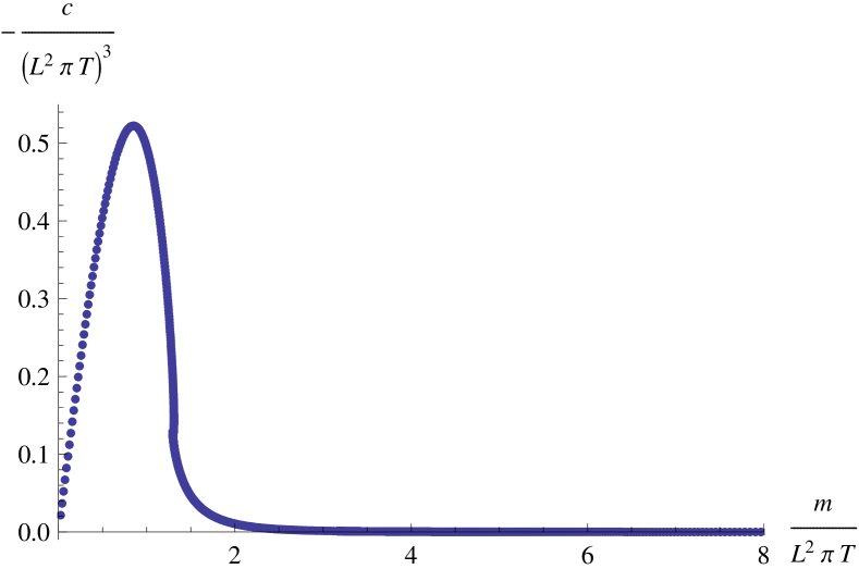
Figure 1: Chiral condensate as function of the quark mass for the static AdS/Schwarzschild background.

Figure 1 shows the chiral condensate as a function of the quark mass for the AdS/Schwarzschild geometry. Since all quantities enter the equations of motion in units of the black hole mass $m_{bh}$ (we express everything in terms of $\pi T=8G_{N}/(3\pi)m_{bh}$), the leading order time-dependence of the chiral condensate can be determined in an adiabatic approximation using the fact that the perfect fluid geometry for constant $\tau$ appears like an AdS/Schwarzschild solution with fixed temperature (17).

Our numerical results provide $c/T^{3}\sim(m/T)^{\alpha}$. $\alpha$ is about $-6$ at $m\approx 3(\pi T)$ and increases to $-5.2$ when going to $m\approx 8(\pi T)$. In other words

$$c\sim\tau^{-(3-\alpha)/3}\approx\tau^{-8.2/3}$$ (25)

However, as has been observed in KarchOBannon , the numerics determining Figure 1 is not particularly accurate for large quark mass because the chiral condensate becomes small. Therefore it is not possible to increase the quark mass till the exponent saturates.

For large quark mass, the solutions are very far from the black hole and become approximately constant embeddings as in the supersymmetric scenario KarchKatz . This suggests the following perturbative analysis Mateos:2007vn . For small $\epsilon$ we seek regular solutions

$$\Phi(\rho) =m+\epsilon f(\rho)$$ (26)

of the DBI action in AdS/Schwarzschild geometry ErdmengerEvans .

$$\mathcal{L}_{D7/AdS/BH} =\rho^{3}\left(1-\frac{\epsilon(L^{2}\pi\,T)^{8}}{16\left(\rho^{2}+\Phi(\rho)^{2}\right)^{4}}\right)\sqrt{1+\Phi^{\prime}(\rho)}$$ (27)

We obtain

$$f(\rho) =-\frac{(L^{2}\pi T)^{8}\left(3m^{4}+3\rho^{2}m^{2}+\rho^{4}\right)}{96m^{5}\left(m^{2}+\rho^{2}\right)^{3}},$$ (28)

$$\implies\frac{c}{(L^{2}\pi T)^{3}} =-\frac{1}{96}\left(\frac{L^{2}\pi T}{m}\right)^{5}.$$ (29)

We have written (29) in a way that emphasizes the known fact that the temperature can be effectively removed from the equations by a suitable redefinition of the quark mass and condensate. In the present context, such a rescaling is not desirable. With (17) we conclude that the adiabatic estimate for the perfect fluid geometry is

$$c =-\frac{\varepsilon_{0}^{2}L^{16}}{54m^{5}}\tau^{-\frac{8}{3}}.$$ (30)

We will check in the following that this is indeed the leading contribution for the expanding plasma geometry.

II.3 Viscous fluid

Restricted to the scalar $\Phi$, the action reads for our geometry (11)

$$S_{D7}=\mathbf{N}\int d\tau\,d\rho\,\tau\,\rho^{3}\,\mathbf{A}\,\sqrt{1+\Phi^{\prime 2}-\mathbf{B}\frac{\dot{\Phi}^{2}}{(\rho^{2}+\Phi^{2})^{2}}},$$ (31)

$$\begin{aligned} \mathbf{A}:=\bigl{(}1-\frac{v^{8}}{9}\bigr{)}&\exp\left[-2\eta_{0}\,\varepsilon_{0}^{-\frac{1}{4}}\frac{v^{8}}{9-v^{8}}\tau^{-\frac{2}{3}}\right],\\ \mathbf{B}:=\frac{1+\frac{v^{4}}{3}}{(1-\frac{v^{4}}{3})^{2}}&\exp\left[2\eta_{0}\,\varepsilon_{0}^{-\frac{1}{4}}v^{4}\frac{9+v^{4}}{9-v^{8}}\tau^{-\frac{2}{3}}\right],\end{aligned}$$ (32)

$$v:=\frac{\varepsilon_{0}^{\frac{1}{4}}L^{2}}{\tau^{\frac{1}{3}}\sqrt{\rho^{2}+\Phi(\rho,\tau)^{2}}},$$ (33)

$$\mathbf{N}:=N_{f}T_{D7}\Omega_{3}V_{x}=\frac{1}{2}\frac{N_{c}N_{f}}{(2\pi\ell_{s}^{2})^{4}\lambda}V_{x},$$ (34)

where $T_{D7}=2\pi/(g_{s}(2\pi\ell_{s})^{8})$ is the D7 tension. $\Omega_{3}=2\pi^{2}$ and $V_{x}=\int dy\,d^{2}x_{\perp}$ are the volume of the unit three-sphere and spatial part of the boundary, respectively. The latter is of course infinite.

Since the viscous fluid geometry discussed in the previous section behaves similar to AdS/Schwarzschild with time-dependent temperature, we do not expect spontaneous symmetry breaking either, though going to small quark masses leaves the domain of validity of the geometry and it is thus hard to make a definite statement. We will therefore only consider ‘Minkowski-type’ embeddings that avoid the horizon at the center of the geometry.

For a given quark mass, in general regularity is only possible for a discrete set of values for the chiral condensate. In the regime under consideration, since no phase transition occurs, we expect $c=c(m)$ to be a one-valued function.

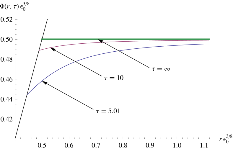
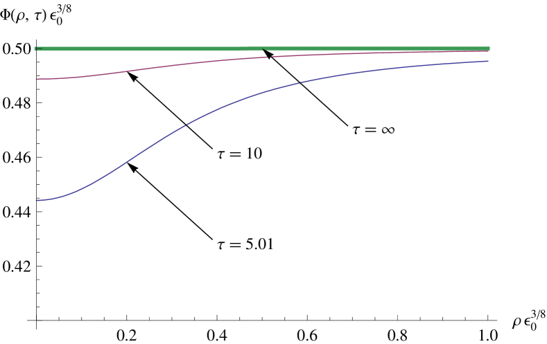
Figure 2: Embeddings with $m=\frac{1}{2}\varepsilon^{-3/8}$ at different times. For late times (bold), the supersymmetric embedding is approximated. The diagonal line in the first plot corresponds to $\Phi(r)\equiv r$, where the embeddings have to end.

The equation of motion arising from (31) is a non-linear partial differential equation. We will solve it perturbatively by a late-time expansion

$$\Phi(\rho,\tau) =m+\sum_{i=1}^{\infty}f_{i}(\rho)\tau^{-\frac{i}{3}}.$$ (35)

We use a fraction of $1/3$ in the exponent because all exponents showing up in the background geometry (11) are integer multiples of one third. The ansatz reduces the equations of motion to the following (infinite) system of ordinary differential equations

$$\rho^{-3}\partial_{\rho}(\rho^{3}f^{\prime}_{i}(\rho))=\mathcal{I}_{i}(\rho)$$ (36)

$$\mathcal{I}_{i}=\frac{8m\varepsilon_{0}^{2}}{9(m^{2}+\rho^{2})^{5}}\cdot\begin{cases}1&\text{if $i=8$}\\ -4\eta_{0}\varepsilon_{0}^{-1/4}&\text{if $i=11$}\\ 0&\text{else; provided $i<14$}\end{cases}$$

The boundary behavior of solutions to (36) is

$$f_{i}(\rho)\xrightarrow[\rho\to\infty]{}m_{i}+\frac{c_{i}}{\rho^{2}},$$ (37)

which becomes an exact solution when the inhomogeneous term vanishes, $\mathcal{I}_{i}=0$. The first term, $m_{i}$, contributes $m_{i}\tau^{-i/3}$ to the bare quark mass. Since we do not accept a time-dependence of the bare parameters on physical grounds, we require $m_{i}=0$. Thus in conjunction with regularity the value of $c_{i}$ is completely fixed. In particular $\mathcal{I}_{i}=0$ implies $c_{i}=0$ or $f_{i}\equiv 0$.

To the considered order the solution is

$$\Phi(\rho,\tau) =m+c\,\frac{\rho^{4}+3\rho^{2}m^{2}+3m^{4}}{(m^{2}+\rho^{2})^{3}},$$ (38)

with

$$c=-\frac{\varepsilon_{0}^{2}L^{16}}{54m^{5}}\tau^{-\frac{8}{3}}\left(1-4\eta_{0}\varepsilon_{0}^{-\frac{1}{4}}\tau^{-\frac{2}{3}}+\dots\right).$$ (39)

In figure 3 we show the effect of the subleading term on the shape of $c(\tau)$. Note that we can trust this result only as long as this term is small compared to the leading order,

$$4\eta_{0}\varepsilon_{0}^{-1/4}\tau^{-2/3} \ll 1.$$ (40)

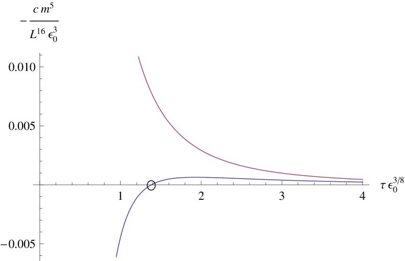
Figure 3: Time-dependence of the chiral condensate for adiabatic approximation (monotonic curve) and with viscosity correction. The circle at $\tau=(4/3)^{9/8}\approx 1.38$ is outside the regime of validity given by equation (40).

We observe that the viscosity term enters the chiral condensate exactly the same way as it enters the energy density squared. We may therefore express the chiral condensate as

$$\langle\mathcal{O}\rangle=\frac{1}{216\pi^{4}}\frac{N_{f}\lambda^{3}}{N_{c}^{3}}\frac{\varepsilon^{2}}{m_{q}^{5}}.$$ (41)

This solution is however only valid for late times as each term in $\varepsilon(\tau)$ apparently diverges for $\tau\to 0$. While at this stage it is not clear up to which time (if at all) our perturbative expansion converges, we may still ask for which range of $\tau$ it is self-consistent. For this consideration, three time-scales are of potential importance. Firstly, the time when the solution touches the horizon, i.e., $\Phi(0,\tau)=3^{-1/4}L^{2}\varepsilon_{0}^{1/3}\tau^{-1/3}$. Secondly, the moment when the viscosity term in the expansion dominates the leading term in such a way that the embedding “recoils” and stops being a one-valued function of the holographic direction $r$. This happens when $d^{2}\Phi(r,\tau)/dr^{2}\to\infty$. Thirdly, the time $\tau=(4/3)^{9/8}\approx 1.38$ when the chiral condensate changes its sign and by (41) would lead to an imaginary energy density. Before this time scale is reached, the regime of validity (40) is left.

For numerical computations and plots, we will use $\varepsilon_{0}^{-3/8}$ (which is a length) as a unit to express dimensionful quantities. Figure 2 shows the $m=1/2\varepsilon_{0}^{-3/8}$ solution at various times before break-down. (Again we would like to stress that the solutions may be invalid even before – by “break-down” we denote their having become invalid for sure.) Figure 4 compares the three effects. For small quark mass solutions are invalidated by touching the horizon, and by imaginary energy density for large quark mass.

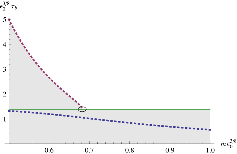
Figure 4: Break-down time of the solution as a function of the quark mass. The horizontal line indicates the time where the energy density becomes imaginary, the dashed flat curve is where embeddings become two-valued as a function of the holographic energy scale $r$ and the steep curve shows where solutions touch the horizon, i.e., can no longer be considered ‘Minkowski-type’. The gray area marks invalid solutions. The circle is at $m\approx 0.682\varepsilon_{0}^{-3/8}$, which is the smallest mass that does not lead to solutions that eventually touch the horizon.

III Meson spectra

In the D3/D7 framework, meson spectra are determined from regular, normalizable solutions to the equations obtained from linearizing the full equations of motion of the D7 brane about the embedding solution that describes the position and shape of the brane KMMW .

In the following section we distinguish between four dimensional meson modes, which carry a “4d” label and eight dimensional fluctuations, which always start with a $\delta$ followed by a (Greek or Latin) capital letter, e.g. $\delta\Phi$ or $\delta A^{y}$. Our ansätze are products of spherical harmonics $\mathcal{Y}$ on the internal manifold, wave forms parallel to the boundary and radial parts, which describe the dependence on the holographic coordinates and are denoted by $\delta$ followed by a small letter.

III.1 Boost invariance for the AdS geometry

Before turning to the actual holographic computation of meson spectra for the viscous fluid, it is insightful to investigate how boost invariance changes wave forms of scalar and vector mesons in the conventional setting, where there is no time-dependence of the meson mass.

In four dimensional Minkowski space the massive Klein–Gordon equation assumes the form

$$\Box\Phi_{4d}=\left[-\frac{1}{\tau}\partial_{\tau}\tau\partial_{\tau}+\tau^{-2}\partial_{y}^{2}+\partial_{x}^{2}\right]\Phi_{4d}=M^{2}\Phi_{4d}$$ (42)

$$\implies\Phi_{4d}=(c_{1}\,\mathrm{J}_{0}(\omega\,\tau)+c_{2}\,\mathrm{Y}_{0}(\omega\,\tau))e^{\pm ik_{\perp}x_{\perp}}$$ (43)

$$k_{\perp}^{2}=k_{2}^{2}+k_{3}^{2}$$

with $\,\mathrm{J}_{0}$ and $\,\mathrm{Y}_{0}$ Bessel functions of first kind. Since a linear combination of the Bessel functions will appear frequently in our expressions we introduce the short hand

$$\mathcal{F}_{p}[\omega]:=c_{1}\,\mathrm{J}_{p}({\textstyle\int}\omega\,d\tau)+c_{2}\,\mathrm{Y}_{p}({\textstyle\int}\omega\,d\tau).$$ (44)

We will not explicitly denote the time-dependence of $\mathcal{F}_{0}$ arising from the integral over $\tau$. At this stage, the integral has been chosen for later convenience and gives $\omega\,\tau$ for constant frequencies. The eigenfrequencies $\omega:=\sqrt{M^{2}+k_{\perp}^{2}}$ are to be determined in our holographic setup. We will thus assume $k_{\perp}=0$ from the start to obtain the mass spectrum.

The 4d meson field is given as the boundary value of (linear, normalizable) fluctuations $\delta\Phi$, $\delta\Psi$ about the embedding solution $\Phi(\rho)\equiv m$,

$$X^{8} =0+\delta\Psi(\rho,\tau), X^{9} =\Phi(\rho)+\delta\Phi(\rho,\tau).$$ (45)

For the presentation of our ansatz, we will concentrate on the scalar mode $\delta\Phi$; the pseudoscalar mode $\delta\Psi$ will be treated analogously. With the following holographic ansatz

$$\delta\Phi(\rho,\tau)=\delta\phi(\rho)\mathcal{F}_{0}[\omega]\mathcal{Y}^{\ell}(S^{3}),$$ (46)

the boundary value corresponding to quantum number $\ell$ is defined by

$$\Phi_{4d}^{(\ell)}=\lim_{\rho\to\infty}\rho^{2}\frac{\delta\Phi(\rho,\tau)}{\mathcal{Y}^{\ell}(S^{3})}$$ (47)

Equation (46) is a natural modification of the ansatz given in KMMW to separate the D7 equation of motion in anti-de Sitter space:

$$\left[-\frac{L^{2}}{(\rho^{2}+m^{2})^{2}}\frac{1}{\tau}\partial_{\tau}\tau\partial_{\tau}+\frac{1}{\rho^{3}}\partial_{\rho}\rho^{3}\partial_{\rho}+\frac{1}{\rho^{2}}\Delta_{S^{3}}\right]\delta\Phi(\rho,\tau)=0.$$ (48)

The radial equation obtained after separation reads

$$\left[\frac{1}{\rho^{3}}\partial_{\rho}\rho^{3}\partial_{\rho}+\frac{L^{2}\omega^{2}}{\rho^{2}+m^{2}}-\frac{\ell(\ell+2)}{\rho^{2}}\right]\delta\phi(\rho)=0,$$ (49)

which is the well-known result of KMMW . For simplicity, we will only consider the lowest Kaluza–Klein mode on the internal $S^{3}$, such that $\ell=0$, $\mathcal{Y}^{0}\equiv 1$.

The requirements of regularity in the interior ($\rho\to 0$) and vanishing at the boundary ($\rho\to\infty$), fix the modes completely. One obtains a discrete set of modes the lightest of which is given by

$$\mathcal{F}_{0}\left[\omega_{0}=\frac{\sqrt{8}m}{L^{2}}\right]\cdot\frac{1}{m^{2}+\rho^{2}}$$ (50)

For a four-dimensional massive vector meson we have

$$\nabla_{a}F^{ab} =M^{2}A_{4d}^{b}.$$ (51)

We assume that the solutions are still plane waves in the $x_{2},x_{3}$-plane, i.e., $A_{4d}^{a}=\xi^{a}(\tau)\exp ik_{\perp}x_{\perp}$. This yields the following component equations

$$-\tau\partial_{\tau}(\frac{1}{\tau}\partial_{\tau}A^{4d}_{y}) =(M^{2}+k_{\perp}^{2})A^{4d}_{y}$$ (52)

$$-\partial_{\tau}^{2}A^{4d}_{2}-\frac{1}{\tau}\partial_{\tau}A^{4d}_{2}+ik_{2} \Bigl{(}\partial_{\tau}+\frac{1}{\tau}\Bigr{)}A^{4d}_{\tau}$$ (53)

$$+k_{2}k_{3}A^{4d}_{3} =(M^{2}+k_{3}^{2})A^{4d}_{2}\qquad\text{and ($2\leftrightarrow 3$)}$$

$$A^{4d}_{\tau} =-\frac{i\partial_{\tau}(k_{2}A^{4d}_{2}+k_{3}A^{4d}_{3})}{\omega^{2}}$$ (54)

Equation (52) can be treated separately. Its solution is

$$A^{4d}_{y} =\tau\mathcal{F}_{1}[\omega]e^{ik_{\perp}x_{\perp}} A^{4d}_{\tau,x^{2},x^{3}} =0.$$ (55)

The others may be solved without loss of generality by turning the coordinate system such that $k_{3}=0$. Then it follows immediately that $A^{4d}_{2,3}=\xi_{2,3}\mathcal{F}_{0}[\omega_{2,3}]\exp ik_{\perp}x_{\perp}$. With this modified ansatz and plugging (54) into (53) we obtain

$$\biggl{[}-M^{2}-k_{3}^{2}+\omega_{2}^{2}\left(1-\frac{k_{2}^{2}}{\omega^{2}}\right)\biggr{]}A^{4d}_{2}+k_{2}k_{3}\biggl{(}1-\frac{\omega_{3}^{2}}{\omega^{2}}\biggr{)}A^{4d}_{3} =0$$

$$\text{and ($2\leftrightarrow 3$)},$$ (56)

which can only be satisfied for $\omega_{2}=\omega_{3}=:\omega_{23}$. Moreover, since it is a homogeneous system, $\omega_{23}(M,k_{2},k_{3})$ can be determined from degeneracy of the coefficient matrix. We shall not reproduce the final expression, but just note that $\omega_{23}=M$ when $k_{2}=k_{3}=0$, which could also have been obtained directly from (53). We thus end up with the two solutions

$$A^{4d}_{2,3}=\xi_{2,3}\mathcal{F}_{0}[\omega_{23}]\exp ik_{\perp}x_{\perp}.$$ (57)

Therefore, we adapt the holographic ansätze for meson modes found in KMMW as follows

Type

I $$\delta A_{\alpha} =\delta a_{I}^{\pm}(\rho)\mathcal{F}_{0}[\omega]e^{ik_{\perp}x_{\perp}}\mathcal{Y}^{\ell,\pm}_{\alpha}(S^{3}),\quad\!\!\alpha=5,6,7;$$

$$\text{II}_{y} \delta A_{y} =\delta a_{IIy}(\rho)\tau\mathcal{F}_{1}[\omega]e^{ik_{\perp}x_{\perp}}\mathcal{Y}^{\ell}(S^{3});$$

$$\text{II}_{2,3}\!\!\! \delta A_{2} =\delta a_{II2}(\rho)\mathcal{F}_{0}[\omega]e^{ik_{\perp}x_{\perp}}\mathcal{Y}^{\ell}(S^{3}),\quad\!\!A_{3}=0;$$

and $$(2\leftrightarrow 3)$$

III $$\delta A_{\rho} =\delta a_{III}(\rho)\mathcal{F}_{0}[\omega]e^{ik_{\perp}x_{\perp}}\mathcal{Y}^{\ell}(S^{3}),$$

$$\delta A_{\alpha} =\delta\tilde{a}_{III}(\rho)\mathcal{F}_{0}[\omega]e^{ik_{\perp}x_{\perp}}\mathcal{Y}^{\ell,\pm}_{\alpha}(S^{3});$$ (58)

with the respective other components set to zero. We will only consider modes of type II, which are the only modes dual to vector mesons and therefore most interesting.

In the ansätze, the dependence in the $0,1,2,3$ directions has been modified as compared to what can be found in KMMW . The reason these changes are straight-forward is the following: The calculation of KMMW only uses two important properties of the ansätze regarding derivatives in those directions,

$$\Delta_{4d}\delta A_{I} =M^{2}\delta A_{I},\qquad I\in[0,\dots,7]$$ (59)

$$g_{4d}^{ab}\partial_{a}\delta A_{b} =0,$$ (60)

where $g_{4d}=\operatorname{diag}(-1,\tau^{2},1,1)$ in our case, whereas in KMMW it was a Minkowski metric. For our ansätze, the gauge condition (60) is either trivially obeyed or follows from (54). Moreover it can be used to turn (59) into (51).

III.2 Viscous fluid geometry

Before coming to the actual holographic computation, we would like to discuss the general framework of late-time perturbative expansions that we use.

Since the viscous fluid geometry and our D7 embeddings are time-dependent, we do not expect, and do not see, a separation into a purely $\tau$ dependent and $\rho$ dependent factor. This makes the problem very difficult to tackle analytically. We are helped by the property that at late proper times the geometry becomes pure $AdS_{5}$ with the corresponding D7 brane embedding. In this limit the simplest solution looks like (50)

$$\mathcal{F}_{0}\left[\omega_{0}=\frac{\sqrt{8}m}{L^{2}}\right]\cdot\frac{1}{m^{2}+\rho^{2}},$$ (61)

where $\mathcal{F}_{0}[\omega]$ is defined in equation (44). For smaller proper-times it is natural to treat the frequency appearing in (61) as depending on $\tau$. However as the equations do not allow for a separation of variables we have $\tau$ dependence also in the remaining part:

$$\tilde{\mathcal{F}}\Bigl{[}\omega(\tau)\Bigr{]}f(\rho,\tau)$$ (62)

where we allow for a general $\tilde{\mathcal{F}}$ which should reduce to $\mathcal{F}_{0}[\omega]$ for constant $\omega$. We have moreover the expansions

$$\omega(\tau) =\omega+\frac{1}{\tau^{\frac{1}{3}}}\omega^{(1)}+\ldots$$ (63)

$$f(\rho,\tau) =f^{(0)}(\rho)+\frac{1}{\tau^{\frac{1}{3}}}f^{(1)}(\rho)+\ldots$$ (64)

Note that the above form is not unique. Redefining the coefficients of the expansions in an appropriate way, we may redefine the split (62). So in order to uniquely specify such an ansatz we have to supplement the usual regularity condition at $\rho=0$ and Dirichlet boundary condition at $\rho=\infty$ by another condition which makes the split (62) unique. In this paper we will impose a condition on the profile of the mode $\delta\phi$ induced on the boundary

$$\Phi_{4d}(\tau)\equiv\lim_{\rho\to\infty}\rho^{2}\delta\phi(\rho,\tau)$$ (65)

Namely we will set

$$\Phi_{4d}(\tau) =\sqrt{\frac{{\textstyle\int}\omega_{4d}(\tau)\,d\tau}{\omega_{4d}\,\tau}}\mathcal{F}_{0}[\omega_{4d}(\tau)].$$ (66)

which provides a definition of our frequency $\omega_{4d}(\tau)$. For constant $\omega_{4d}(\tau)$ this reduces of course to the pure $AdS_{5}$ result (61).

Our motivation for the above form (66) is that it arises as a WKB approximation to a Klein–Gordon equation with time dependent mass spectra:

$$\Box\Phi_{4d} =\left[-\frac{1}{\tau}\partial_{\tau}\tau\partial_{\tau}+\tau^{-2}\partial_{y}^{2}+\partial_{x}^{2}\right]\Phi_{4d}=M^{2}_{4d}(\tau)\Phi_{4d}$$ (67)

We may separate variables by assuming a plane wave in the $2,3$ plane and obtain $\omega_{4d}^{2}(\tau)=M_{4d}^{2}(\tau)+k_{\perp}^{2}$. (Though we will assume $k_{\perp}=0$, henceforth.) The remaining equation

$$-\frac{1}{\tau}\partial_{\tau}\tau\partial_{\tau}\Phi_{4d}(\tau)=\omega^{2}_{4d}(\tau)\Phi_{4d}(\tau)$$ (68)

can only be solved approximately, e.g., by the WKB approximation, which gives two linearly independent solutions,

$$\Phi_{4d}(\tau) \approx\sqrt{\frac{{\textstyle\int}\omega_{4d}(\tau)\,d\tau}{\omega_{4d}\,\tau}}\mathcal{F}_{0}[\omega_{4d}(\tau)].$$ (69)

The square root prefactor ensures that Abel’s theorem is fulfilled, such that the Wronskian for our ansatz is

$$W=\frac{\text{const}}{t}$$ (70)

as it should be for the exact solution.

We have now all ingredients in place to actually calculate the meson spectrum for the time-dependent viscous fluid geometry. We expand the D7 action (II.1), given by

$$\mathcal{L}_{DBI} =e^{\frac{\mathcal{A}}{2}+\frac{\mathcal{B}}{2}+\mathcal{C}}\rho^{3}\tau\biggl{[}1+(\partial_{\rho}X^{9})^{2}+(\partial_{\rho}X^{8})^{2}+e^{-\mathcal{C}}(\partial_{\rho}A_{2}){}^{2}$$

$$\qquad\qquad+\frac{e^{-\mathcal{B}}}{\tau^{2}}(\partial_{\rho}A_{y}){}^{2}-\frac{e^{-\mathcal{A}}L^{4}}{r^{4}}(\text{I})+\text{(quartic)}\biggr{]}^{1/2}$$

$$(\text{I}) =(\partial_{\tau}X^{8})^{2}+(\partial_{\tau}X^{9})^{2}+(\partial_{\rho}X^{8})^{2}(\partial_{\tau}X^{9})^{2}$$

$$\qquad+(\partial_{\tau}X^{8})^{2}(\partial_{\rho}X^{9})^{2}$$

$$\qquad-2(\partial_{\tau}X^{8})(\partial_{\rho}X^{9})(\partial_{\rho}X^{8})(\partial_{\tau}X^{9})$$

$$\qquad+e^{-\mathcal{C}}(\text{II})+\frac{e^{-\mathcal{B}}}{\tau^{2}}(\text{III})$$ (71)

$$(\text{II}) =(\partial_{\tau}A_{2}){}^{2}+(\partial_{\rho}X^{9})^{2}(\partial_{\tau}A_{2}){}^{2}+(\partial_{\tau}X^{9})^{2}(\partial_{\rho}A_{2}){}^{2}$$

$$\qquad-2(\partial_{\tau}X^{9})(\partial_{\rho}X^{9})(\partial_{\rho}A_{2})(\partial_{\tau}A_{2})$$ (72)

$$(\text{III}) =+(\partial_{\tau}A_{y}){}^{2}+(\partial_{\rho}X^{9})^{2}(\partial_{\tau}A_{y}){}^{2}+(\partial_{\tau}X^{9})^{2}(\partial_{\rho}A_{y}){}^{2}$$

$$\qquad-2(\partial_{\tau}X^{9})(\partial_{\rho}X^{9})(\partial_{\rho}A_{y})(\partial_{\tau}A_{y})$$ (73)

to quadratic order in fluctuations

$$X^{9} =\Phi+\delta\Phi, X^{8} =0+\delta\Psi,$$

$$A_{2} =0+\delta A_{2}, A_{y} =0+\delta A_{y}.$$ (74)

The resulting equation of motion is evaluated by performing a perturbative expansion in $\tau^{-1/3}$,

$$\delta\Phi =c_{1}\,\mathrm{J}_{0}\Bigl{(}{\textstyle\int}\omega^{(\phi)}(\tau)\,d\tau\Bigr{)}\sum_{j=0}^{\infty}\delta\phi_{j}(\rho)\,\tau^{-j/3}$$

$$+c_{2}\,\mathrm{Y}_{0}\Bigl{(}{\textstyle\int}\omega^{(\phi)}(\tau)\,d\tau\Bigr{)}\sum_{j=0}^{\infty}\delta\tilde{\phi}_{j}(\rho)\,\tau^{-j/3},$$ (75)

$$\omega^{(\phi)} =\sum_{i=0}^{\infty}\omega_{i}\,\tau^{-\frac{i}{3}},$$ (76)

and analogously for the other fluctuations. We use the known asymptotic expansion of the Bessel functions and obtain schematically the following equation

$$[\text{polynomial in $\tau^{-1/3}$}]\cos\bigl{(}{\textstyle\int}\omega^{(\phi)}\,d\tau\bigr{)}$$

$$\qquad\qquad+[\text{polynomial in $\tau^{-1/3}$}]\sin\bigl{(}{\textstyle\int}\omega^{(\phi)}\,d\tau\bigr{)}=0.$$ (77)

At any given order, the requirement that the coefficients of the polynomials vanish, provides a differential equation for $\delta\phi_{i}$ and $\delta\tilde{\phi}_{i}$ depending on $\omega_{i}$ (and lower order solutions). We have to go to order 6 before the viscosity $\eta_{0}$ enters the equations. To this order, the equations for $\delta\phi_{i}$ and $\delta\tilde{\phi}_{i}$ can be separated by choosing suitable linear combinations and yield $\delta\phi_{i}\equiv\delta\tilde{\phi}_{i}$, which is what is required for the WKB ansatz (69) to be applicable. We impose the boundary conditions

$$\delta\phi\xrightarrow[\rho\to\infty]{}0,\qquad\delta\phi\xrightarrow[\rho\to 0]{}\text{finite},$$

$$\rho^{2}\delta\phi\xrightarrow[\rho\to\infty]{}\sqrt{\frac{{\textstyle\int}\omega^{(\phi)}\,d\tau}{\omega^{(\phi)}\tau}}\mathcal{F}_{0}[\omega^{(\phi)}].$$ (78)

The first two of these conditions pick regular normalizable solutions; the last ensures that meson solutions on the boundary (65) satisfy the constraint (70). Consequently, the conditions fix two integration constants and the frequency $\omega_{i}$ at each order in the perturbative expansion. The only remaining free constants are the overall factors $c_{1}$ and $c_{2}$ of our ansatz (III.2).

Each of the coefficient functions has to satisfy a differential equation that is best expressed with the substitutions

$$\delta\phi_{i}(\rho) =(1-\mathbf{y})^{-n-1}\delta\phi_{i}(\mathbf{y}),$$

$$\mathbf{y} =-\rho^{2}/m^{2},$$ (79)

$$\omega_{0}^{2} =m^{2}((2n+3)^{2}-1).$$

The lowest order equation then reads

$$\begin{gathered}\left[\mathbf{y}(1-\mathbf{y})\partial_{\mathbf{y}}^{2}+(\mathbf{c}-(\mathbf{a}+\mathbf{b}-1)\mathbf{y})\partial_{\mathbf{y}}-\mathbf{a}\,\mathbf{b}\right]\phi_{0}(\mathbf{y})=0\\ \mathbf{a}=-n-1,\qquad\mathbf{b}=-n,\qquad\mathbf{c}=2.\end{gathered}$$ (80)

This is exactly the hypergeometric equation already encountered in KMMW . The boundary conditions fix $n$ to be a non-negative integer, thus yielding a discrete meson spectrum $M=\omega_{0}(n)$ and the solutions in terms of (degenerate) hypergeometric functions $\operatorname{{}_{2}F_{1}}$ are

$$h_{1} =\operatorname{{}_{2}F_{1}}(-n-1,-n,2;\mathbf{y}),$$ (81)

$$h_{2} =(1-\mathbf{y})^{3+2n}\operatorname{{}_{2}F_{1}}(n+2,n+3,2n+4;1-\mathbf{y}).$$ (82)

Only $h_{1}$ is regular, such that $\delta\phi_{0}\equiv h_{1}$.

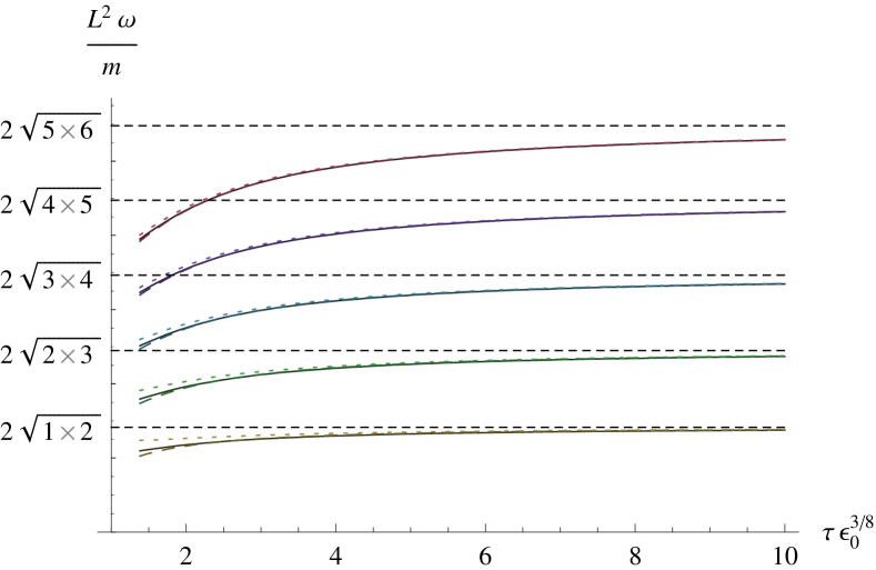
Figure 5: Late-time spectra for the viscous fluid geometry. The supersymmetric spectrum is shown as dashed horizontal lines. Scalar mesons are shown as continuous lines, vector modes are dashed.

Higher orders in perturbation theory produce inhomogeneous terms in the analogues of (80). Since it is a linear ordinary equation, the solution can still be obtained in closed form by standard methods. However, the resulting integrals are hard to solve in general. Since both solutions $h_{1,2}$ are rational functions of $\mathbf{y}$ and $\ln\mathbf{y}$, it is however easy to do so for definite $n$. For the lowest five mesons $n=0,\dots,4$ we give the solutions in the appendix.

The mass of the lowest scalar meson mode is

$$\omega^{(\phi)}=\tfrac{4\pi}{\sqrt{\lambda}}\cdot\left[m_{q}-\tfrac{3\lambda^{2}\varepsilon_{0}}{80\pi^{4}\tau^{4/3}m_{q}^{3}}\cdot\left(1-\tfrac{2\eta_{0}}{\tau^{\frac{2}{3}}\varepsilon_{0}^{\frac{1}{4}}}\right)\right].$$ (83)

To the considered order, pseudoscalar modes $\delta\psi$ have exactly the same equations of motion and the spectrum is degenerate. Moreover we note that the spectrum agrees with the adiabatic approximation even including the viscosity corrections. The reason for this might be that the bulk metric coefficients that enter the calculation for the scalar mesons can be expressed completely in terms of the energy density, whereas the components for the $y,2,3$ directions cannot.

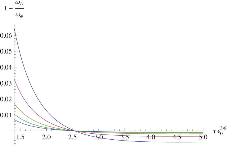
Figure 7: The plot shows the relative difference of the masses of (type II_y) vector and scalar mesons for $m=\varepsilon_{0}^{3/8}$.

The vector mesons deviate slightly from the scalar modes. For comparison we plot the mass ratio of scalar and vector modes in Figure 7. The mass of the lowest vector mesons is given by

$$\omega^{(A^{y})}=\tfrac{4\pi}{\sqrt{\lambda}}\cdot\left[m_{q}-\tfrac{7\lambda^{2}\varepsilon_{0}}{240\pi^{4}\tau^{4/3}m_{q}^{3}}\cdot\left(1-\tfrac{6\eta_{0}}{7\tau^{\frac{2}{3}}\varepsilon_{0}^{\frac{1}{4}}}\right)\right],$$ (84)

$$\omega^{(A^{2,3})}=\tfrac{4\pi}{\sqrt{\lambda}}\cdot\left[m_{q}-\tfrac{7\lambda^{2}\varepsilon_{0}}{240\pi^{4}\tau^{4/3}m_{q}^{3}}\cdot\left(1-\tfrac{18\eta_{0}}{7\tau^{\frac{2}{3}}\varepsilon_{0}^{\frac{1}{4}}}\right)\right].$$ (85)

This agrees with the adiabatic approximation excluding the viscosity term. Since the metric components that enter the holographic computation, $g_{yy}$ and $g_{22}$, agree only up to the viscosity terms, this deviation does not come as a surprise.

We plot the five lowest meson modes in Figure 5. The leading order term gives the exact supersymmetric spectrum that is approached for $\tau\to\infty$.

III.3 Comparison to the adiabatic approximation

In this subsection, we will review some properties of low-temperature meson spectra for the static AdS black hole. Plugging in the time-dependence of the temperature into the static meson spectra, yields an estimate for the time-dependent spectrum, which we will refer to as adiabatic approximation. We will assume that the temperature dependence given in terms of Poincaré time $t$ can be obtained from (17) by substituting $\tau$ for $t$:

$$T_{AdS/BH}(t)=\left(\frac{4\varepsilon_{0}}{3}\right)^{\frac{1}{4}}\frac{1}{\pi\,t^{\frac{1}{3}}}\left[1-\frac{\eta_{0}}{2\varepsilon_{0}^{1/4}t^{2/3}}\right].$$ (86)

Note however that we do not expect the resulting adiabatic meson spectra to accurately give the viscosity corrections. The reason for this is that even though the horizon position can be expressed completely in terms of the energy density, such that the Stefan–Boltzmann law holds, the bulk metric and energy momentum tensor nevertheless contain additional viscosity terms that cannot be captured by the AdS/Schwarzschild geometry even when the geometry near the horizon and near the boundary is matched.

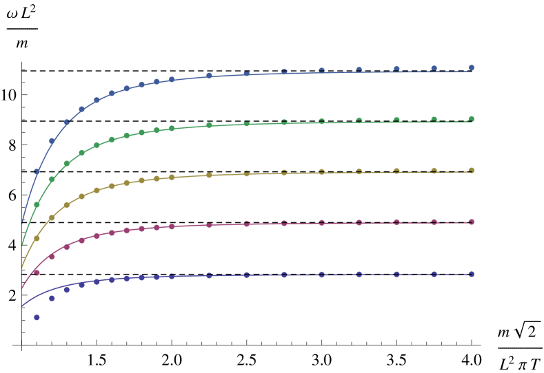
Figure 6: The plot shows the (pseudo)scalar meson spectrum. For small temperatures, the supersymmetric spectrum (dashed) is approached. The solid lines are asymptotic $T\to 0$ solutions, which are in good agreement with the numerical solutions (dots) for small temperatures.

In Figure 6 we plot the numerical solution (dots) of the static case. We calculate the asymptotic solution in a low temperature expansion (solid curves), which agrees with the numerical calculation. Plugging the time dependence of the temperature (86) into this analytical approximation, we obtain the time-dependent meson spectrum in adiabatic approximation. The mass of the lowest scalar and vector modes are given by

$$\omega_{\phi,\psi}^{\text{ad.}} =\frac{4\pi}{\sqrt{\lambda}}\left[m_{q}-\frac{9\lambda^{2}}{320}\frac{T^{4}}{m_{q}^{3}}\right]$$

$$=\frac{4\pi}{\sqrt{\lambda}}\left[m_{q}-\frac{3\lambda^{2}}{80\pi^{4}}\frac{\varepsilon_{0}}{m_{q}^{3}}t^{-\frac{4}{3}}\left(1-\tfrac{2\eta_{0}}{t^{\frac{2}{3}}\varepsilon_{0}^{\frac{1}{4}}}\right)\right],$$ (87)

$$\omega_{A^{\mu}}^{\text{ad.}} =\frac{4\pi}{\sqrt{\lambda}}\left[m_{q}-\frac{7\lambda^{2}}{320}\frac{T^{4}}{m_{q}^{3}}\right]$$

$$=\frac{4\pi}{\sqrt{\lambda}}\left[m_{q}-\frac{7\lambda^{2}}{240\pi^{4}}\frac{\varepsilon_{0}}{m_{q}^{3}}t^{-\frac{4}{3}}\left(1-\tfrac{2\eta_{0}}{t^{\frac{2}{3}}\varepsilon_{0}^{\frac{1}{4}}}\right)\right].$$ (88)

The mass of all of these modes decreases for increasing temperature. Moreover, the adiabatic scalar modes completely agree with our result (83), whereas the vector modes only agree in the leading contribution; the viscosity terms differ. We consider the agreement of the scalars accidental in the sense that it is a consequence of a certain property of the expanding plasma geometry: All metric coefficients entering the scalar equation of motion can be expressed purely in terms of the temperature, while additional viscosity terms only show up in those metric coefficients that end up in the equations for the vector modes.

An important assumption in our calculation has been that the Klein–Gordon equation is obeyed by scalar particles. This assumption can actually be proved employing the holographic equation of motion resulting from the linearization procedure. There is a parity symmetry $\rho\mapsto-\rho$ in the equation of motion. Since only ‘Minkowski-type’ solutions are considered, this will lead to even solutions, which have the following expansion,

$$\delta\Phi(\rho\to\infty,\tau) \sim\Phi_{4d}(\tau)\frac{1}{\rho^{2}}-\frac{L^{4}\Phi_{4d}(\tau)}{8}M^{2}(\tau)\frac{1}{\rho^{4}}+\dots,$$ (89)

because only normalizable solutions are allowed, such that the constant leading term vanishes. The subleading coefficient $M^{2}(\tau)$ has been multiplied by an additional factor $-L^{4}\Phi_{4d}/8$ for later convenience. Plugging above expansion into the eight-dimensional equation of motion, yields at leading order in $1/\rho$,

$$-\frac{1}{\tau}\partial_{\tau}(\tau\partial_{\tau})\Phi_{4d} =M^{2}(\tau)\Phi_{4d}.$$ (90)

This establishes that at least for a background geometry dual to a hydrodynamic expansion up to and including viscosity, the scalar meson equation is a Klein–Gordon equation with time-dependent mass. This might change when also encoding higher order effects like the relaxation time Heller:2007qt , which currently appears to be out of reach of a supergravity approximation Benincasa:2007tp .

We will now assess the error of the WKB approximation by plugging our meson solutions into the four dimensional Klein–Gordon equation. The error should be smaller than $\tau^{-2}$ to be subleading to the viscosity contribution. We first determine the four dimensional meson solution by

$$\Phi_{4d}^{(\ell)} =\lim_{\rho\to\infty}\rho^{2}\delta\phi(\rho,\tau)\mathcal{F}_{0}[\omega^{(\phi)}]$$ (91)

where on the right hand side we plug in the mass (83) of the lowest holographic scalar meson solution, i.e., we set $\omega_{4d}\approx\omega^{(\phi)}$.

With (91) the error estimate $\Delta\omega$ can be obtained from the Klein–Gordon equation

$$\frac{1}{\tau}\partial_{\tau}\tau\partial_{\tau}\Phi_{4d}(\tau)=\bigl{(}\omega^{(\phi)}(\tau)+\Delta\omega(\tau)\bigr{)}^{2}\Phi_{4d}(\tau),$$ (92)

by linearizing in $\Delta\omega$. This yields

$$\Delta\omega(\tau)=\frac{\sqrt{2}L^{10}\varepsilon_{0}}{5m^{4}}\frac{1}{\tau^{10/3}}+\dots,$$ (93)

which is sufficiently small, that is subleading to the viscosity terms arising from the geometry. (Also note that the frequencies $\omega^{(\phi)}(\tau)$ and the meson mass obtained from the holographic expansion (89) agree up to and including order $\tau^{-2}$.) However when encoding hydrodynamic effects in the geometry that are of sufficiently high order, we would be forced to consider a better approximation for our ansatz, e.g., by using higher order WKB. Moreover, beyond a certain order the WKB ansatz is expected not to work anymore because the coefficients $\delta\phi_{i}$ and $\delta\tilde{\phi}$ are not expected to coincide to arbitrary order.

IV Regularized D7 action

In the static case, the free energy density can be related to the regularized D7 action by means of a Wick rotation. In the conventions of Mateos:2007vn the time direction is periodically identified with $\beta=1/T$, such that the free energy density $F$ is given by

$$F =T\cdot\frac{S_{D7}}{V_{x}},$$ (94)

with $T$ the temperature and $V_{x}=\int d^{3}x$ the (infinite) spatial volume of the boundary. The authors of Mateos:2007vn obtain

$$\frac{S_{D7}}{V_{x}} \sim-\frac{N_{c}N_{f}T^{3}\lambda}{32}\cdot\frac{1}{12}\left(\frac{T}{2m_{q}/\sqrt{\lambda}}\right)^{4}=-\frac{N_{c}N_{f}\lambda^{3}}{6114m_{q}^{4}}\,T^{7}$$ (95)

in the limit of low temperature. While it is clear that for a time-dependent background neither $1/T=\int dt$ nor (94) really make sense, we are still interested in how our action relates to above asymptotic result.

When calculating the action $S_{D7}$, the integration along the holographic direction $\rho$ on the brane is encumbered by UV divergences. The standard procedure of holographic renormalization for the case of a probe D7 brane has been worked out in Karch:2005ms . It consists in regularization by introducing a cut off $\rho_{max}$ and addition of suitable counterterms formed from the induced metric and corresponding curvature on the slice $\rho=\rho_{max}$.

$$S_{reg} =\int\limits_{0}^{\rho_{max}}\mathcal{L}_{D7}\,d\rho+\sum L_{i}(\rho_{max})$$ (96)

To be more precise, the procedure is usually formulated in terms of the coordinate

$$z =(\rho^{2}+\Phi^{2})^{-1/2},$$ (97)

where the counterterms $L_{i}$ read

$$\begin{aligned} L_{1}&=-\frac{1}{4}\sqrt{\gamma}\\ L_{2}&=-\frac{1}{48}\sqrt{\gamma}R_{\gamma}\\ L_{3}&=-\ln(z_{min})\sqrt{\gamma}\frac{1}{32}(R_{ij}R^{ij}-\frac{1}{3}R_{\gamma})\\ L_{4}&=\frac{1}{2}\sqrt{\gamma}\Psi^{2}\\ L_{5}&=-\frac{1}{2}\ln(z_{min})\Psi(\partial_{\tau}\gamma^{\tau\tau}\sqrt{\gamma}\partial_{\tau}+\frac{1}{6}\sqrt{\gamma}R_{\gamma})\Psi\\ L_{f}&=\alpha\gamma\Psi^{4}\end{aligned}$$ (98)

$L_{f}$ is a finite counter term, with an arbitrary parameter $\alpha$, that corresponds to different renormalization schemes. It can be fixed in supersymmetric settings by the requirement that the free energy vanishes. $\gamma$ is the induced metric on the $z=z_{min}$ slice and

$$\Psi =\arcsin\left(\frac{z\Phi}{L^{2}}\right)$$ (99)

is the embedding coordinate of the D7 expressed as an angle on the internal $S^{5}$.

We express the counterterms in terms of $\rho_{max}:=(z_{min}^{-2}-\Phi^{2}(\rho_{max}))^{-1/2}$ using equations (99) and (97)

$$\sum L_{i} =-\frac{1}{4}\tau\rho_{max}^{4}+\tau m^{4}\frac{5+12\alpha}{12}+\mathcal{O}\bigl{(}\rho_{max}^{-1}\bigr{)}$$ (100)

As a check we turn this back into $z$ coordinates by self-consistently iterating (97)

$$\rho_{max}^{2} =\sqrt{z_{min}^{-2}+\Phi^{2}\left(\sqrt{z_{min}^{-2}+\Phi^{2}\left(\sqrt{z_{min}^{-2}+\Phi^{2}\left(\dots\right)}\right)}\right)}$$ (101)

and using the D7 embedding (38). We obtain

$$\frac{1}{\tau}\sum L_{i} =-\frac{1}{4}(m^{2}-z_{min}^{-2})^{2}-4m\,c+\frac{m^{4}(5+12\alpha)}{12},$$ (102)

which up to the $\tau$-dependence arising from our rapidity coordinates is exactly the result of Mateos:2007vn , eq. (4.21), for $\alpha=-5/12$.

The renormalized action is thus

$$S_{ren}=\mathbf{N}\int d\tau\lim_{\rho_{max}\to\infty}\int\limits_{0}^{\rho_{max}}(\mathcal{L}_{DBI}-\rho^{3}\tau)\,d\rho\qquad$$

$$+\frac{1}{12}m^{4}(5+12\alpha)\tau,$$ (103)

where the last two terms are the divergent part of the counterterm, suitably rewritten as an integral, and the remaining finite part. Of course due to the renormalization, the limit can actually be carried out. For late times we obtain

$$S_{ren} =\mathbf{N}\int d\tau\,\tau\left[\frac{m^{4}}{12}(12\alpha+5)-\frac{\varepsilon_{0}^{2}L^{16}}{108m^{4}\tau^{8/3}}+\frac{\varepsilon_{0}^{7/4}\eta_{0}L^{16}}{27m^{4}\tau^{10/3}}\right]$$ (104)

such that for $\alpha=-5/12$ the configuration indeed relaxes to the supersymmetric setting.

The above is our result. For comparison with (95) we perform an additional, somewhat ill-defined step, namely replacing $\int d\tau\,\tau\mapsto 1/T$. With $L^{4}=2\lambda\ell_{s}^{4}$ and equation (34) we obtain for the supersymmetric scheme

$$S_{ren} =-\frac{1}{3\cdot 2^{11}}\frac{N_{c}N_{f}\lambda^{3}}{m_{q}^{4}}\,T^{7},$$ (105)

which agrees with (95).

V Conclusions

The main goal of this article was to study fundamental fields in the holographic dual of an expanding viscous fluid. The dual geometry has strong similarity to a black hole geometry with time-dependent temperature. Small temperatures correspond to late-times. We determined the D7 embedding and calculated the consequences of dynamical temperature for the chiral condensate to three orders. The leading order gives the supersymmetric solution, the subleading corresponds to the adiabatic approximation and the subsubleading order includes viscosity corrections going beyond the adiabatic approximation.

Moreover we calculated the meson spectrum and find that it agrees in the subleading order, though only the scalar mesons agree in the subsubleading order with the adiabatic approximation. The agreement crucially depends on the choice of ansatz defining the frequencies. We demonstrate that for our WKB ansatz solves the Klein–Gordon up to an error smaller than that inescapably introduced in the late-time expansion of the geometry.

However, for the next order, which introduces the relaxation time Heller:2007qt , higher order terms would be needed in the WKB approximation in order to still keep that error smaller than the geometry’s.

It would be interesting to consider analogous properties for gauge theories which exhibit chiral symmetry breaking and hence are more closer to QCD. However up till now there is no description of an expanding plasma system in such a theory.

Appendix A Meson solutions

(Pseudo-)scalar mesons

$$\delta\Phi_{0} =\mathcal{F}_{0}[\omega_{0}]\biggl{[}\tfrac{\left(8m^{4}+9\rho^{2}m^{2}+3\rho^{4}\right)\varepsilon_{0}L^{8}}{10m^{4}\left(m^{2}+\rho^{2}\right)^{3}\tau^{4/3}}-\tfrac{\left(13m^{4}+12\rho^{2}m^{2}+3\rho^{4}\right)\varepsilon_{0}^{3/4}\eta_{0}L^{8}}{10m^{4}\left(m^{2}+\rho^{2}\right)^{3}\tau^{2}}+\tfrac{1}{m^{2}+\rho^{2}}\biggr{]},$$

$$\omega_{0} =\tfrac{2\sqrt{2}m}{L^{2}}+\left(-\tfrac{3L^{6}\tau^{-4/3}\varepsilon_{0}}{5\sqrt{2}m^{3}}\right)\times\left(1-\tfrac{2\eta_{0}}{\tau^{2/3}\sqrt[4]{\varepsilon_{0}}}\right),$$

$$\delta\Phi_{1} =\mathcal{F}_{0}[\omega_{1}]\biggl{[}\tfrac{\left(-12m^{6}+15\rho^{2}m^{4}+20\rho^{4}m^{2}+5\rho^{6}\right)\varepsilon_{0}L^{8}}{14m^{4}\left(m^{2}+\rho^{2}\right)^{4}\tau^{4/3}}+\tfrac{\left(19m^{6}-35\rho^{2}m^{4}-35\rho^{4}m^{2}-5\rho^{6}\right)\varepsilon_{0}^{3/4}\eta_{0}L^{8}}{14m^{4}\left(m^{2}+\rho^{2}\right)^{4}\tau^{2}}+\tfrac{\rho^{2}-m^{2}}{\left(m^{2}+\rho^{2}\right)^{2}}\biggr{]},$$

$$\omega_{1} =\tfrac{2\sqrt{6}m}{L^{2}}+\left(-\tfrac{5\sqrt{3}L^{6}\tau^{-4/3}\varepsilon_{0}}{7\sqrt{2}m^{3}}\right)\times\left(1-\tfrac{2\eta_{0}}{\tau^{2/3}\sqrt[4]{\varepsilon_{0}}}\right),$$

$$\delta\Phi_{2} =\mathcal{F}_{0}[\omega_{2}]\biggl{[}\tfrac{\left(26m^{8}-140\rho^{2}m^{6}-22\rho^{4}m^{4}+55\rho^{6}m^{2}+11\rho^{8}\right)\varepsilon_{0}L^{8}}{30m^{4}\left(m^{2}+\rho^{2}\right)^{5}\tau^{4/3}}$$

$$\qquad\qquad\qquad-\tfrac{\left(41m^{8}-269\rho^{2}m^{6}+121\rho^{6}m^{2}+11\rho^{8}\right)\varepsilon_{0}^{3/4}\eta_{0}L^{8}}{30m^{4}\left(m^{2}+\rho^{2}\right)^{5}\tau^{2}}+\tfrac{m^{4}-3\rho^{2}m^{2}+\rho^{4}}{\left(m^{2}+\rho^{2}\right)^{3}}\biggr{]},$$

$$\omega_{2} =\tfrac{4\sqrt{3}m}{L^{2}}+\left(-\tfrac{11L^{6}\tau^{-4/3}\varepsilon_{0}}{5\sqrt{3}m^{3}}\right)\times\left(1-\tfrac{2\eta_{0}}{\tau^{2/3}\sqrt[4]{\varepsilon_{0}}}\right),$$

$$\delta\Phi_{3} =\mathcal{F}_{0}[\omega_{3}]\biggl{[}\tfrac{\left(-134m^{10}+1506\rho^{2}m^{8}-1650\rho^{4}m^{6}-1045\rho^{6}m^{4}+342\rho^{8}m^{2}+57\rho^{10}\right)\varepsilon_{0}L^{8}}{154m^{4}\left(m^{2}+\rho^{2}\right)^{6}\tau^{4/3}}$$

$$\qquad\qquad\qquad+\tfrac{\left(211m^{10}-2784\rho^{2}m^{8}+3585\rho^{4}m^{6}+1805\rho^{6}m^{4}-912\rho^{8}m^{2}-57\rho^{10}\right)\varepsilon_{0}^{3/4}\eta_{0}L^{8}}{154m^{4}\left(m^{2}+\rho^{2}\right)^{6}\tau^{2}}$$

$$\qquad\qquad\qquad+\tfrac{-m^{6}+6\rho^{2}m^{4}-6\rho^{4}m^{2}+\rho^{6}}{\left(m^{2}+\rho^{2}\right)^{4}}\biggr{]},$$

$$\omega_{3} =\tfrac{4\sqrt{5}m}{L^{2}}+\left(-\tfrac{57\sqrt{5}L^{6}\tau^{-4/3}\varepsilon_{0}}{77m^{3}}\right)\times\left(1-\tfrac{2\eta_{0}}{\tau^{2/3}\sqrt[4]{\varepsilon_{0}}}\right),$$

$$\delta\Phi_{4} =\mathcal{F}_{0}[\omega_{4}]\biggl{[}\tfrac{\left(68m^{12}-1279\rho^{2}m^{10}+3543\rho^{4}m^{8}-630\rho^{6}m^{6}-1566\rho^{8}m^{4}+203\rho^{10}m^{2}+29\rho^{12}\right)\varepsilon_{0}L^{8}}{78m^{4}\left(m^{2}+\rho^{2}\right)^{7}\tau^{4/3}}$$

$$\qquad\qquad\qquad-\tfrac{\left(107m^{12}-2326\rho^{2}m^{10}+7057\rho^{4}m^{8}-1840\rho^{6}m^{6}-3161\rho^{8}m^{4}+638\rho^{10}m^{2}+29\rho^{12}\right)\varepsilon_{0}^{3/4}\eta_{0}L^{8}}{78m^{4}\left(m^{2}+\rho^{2}\right)^{7}\tau^{2}}$$

$$\qquad\qquad\qquad+\tfrac{m^{8}-10\rho^{2}m^{6}+20\rho^{4}m^{4}-10\rho^{6}m^{2}+\rho^{8}}{\left(m^{2}+\rho^{2}\right)^{5}}\biggr{]},$$

$$\omega_{4} =\tfrac{2\sqrt{30}m}{L^{2}}+\left(-\tfrac{29\sqrt{\tfrac{5}{6}}L^{6}\tau^{-4/3}\varepsilon_{0}}{13m^{3}}\right)\times\left(1-\tfrac{2\eta_{0}}{\tau^{2/3}\sqrt[4]{\varepsilon_{0}}}\right)$$

Vector meson (Type II_2,3)

$$(\delta a_{II2})_{0} =\mathcal{F}_{0}[\omega_{0}]\biggl{[}\tfrac{\left(22m^{4}+21\rho^{2}m^{2}+7\rho^{4}\right)\varepsilon_{0}L^{8}}{30m^{4}\left(m^{2}+\rho^{2}\right)^{3}\tau^{4/3}}-\tfrac{\left(13m^{4}+12\rho^{2}m^{2}+3\rho^{4}\right)\varepsilon_{0}^{3/4}\eta_{0}L^{8}}{10m^{4}\left(m^{2}+\rho^{2}\right)^{3}\tau^{2}}+\tfrac{1}{m^{2}+\rho^{2}}\biggr{]},$$

$$\omega_{0} =\tfrac{2\sqrt{2}m}{L^{2}}+\left(-\tfrac{7L^{6}\tau^{-4/3}\varepsilon_{0}}{15\sqrt{2}m^{3}}\right)\times\left(1-\tfrac{18\eta_{0}}{7\tau^{2/3}\sqrt[4]{\varepsilon_{0}}}\right),$$

$$(\delta a_{II2})_{1} =\mathcal{F}_{0}[\omega_{1}]\biggl{[}\tfrac{\left(-118m^{6}+137\rho^{2}m^{4}+164\rho^{4}m^{2}+41\rho^{6}\right)\varepsilon_{0}L^{8}}{126m^{4}\left(m^{2}+\rho^{2}\right)^{4}\tau^{4/3}}$$

$$\qquad\qquad\qquad+\tfrac{\left(19m^{6}-35\rho^{2}m^{4}-35\rho^{4}m^{2}-5\rho^{6}\right)\varepsilon_{0}^{3/4}\eta_{0}L^{8}}{14m^{4}\left(m^{2}+\rho^{2}\right)^{4}\tau^{2}}+\tfrac{\rho^{2}-m^{2}}{\left(m^{2}+\rho^{2}\right)^{2}}\biggr{]},$$

$$\omega_{1} =\tfrac{2\sqrt{6}m}{L^{2}}+\left(-\tfrac{41L^{6}\tau^{-4/3}\varepsilon_{0}}{21\sqrt{6}m^{3}}\right)\times\left(1-\tfrac{90\eta_{0}}{41\tau^{2/3}\sqrt[4]{\varepsilon_{0}}}\right),$$

$$(\delta a_{II2})_{2} =\mathcal{F}_{0}[\omega_{2}]\biggl{[}\tfrac{\left(178m^{8}-880\rho^{2}m^{6}-106\rho^{4}m^{4}+315\rho^{6}m^{2}+63\rho^{8}\right)\varepsilon_{0}L^{8}}{180m^{4}\left(m^{2}+\rho^{2}\right)^{5}\tau^{4/3}}$$

$$\qquad\qquad\qquad-\tfrac{\left(41m^{8}-269\rho^{2}m^{6}+121\rho^{6}m^{2}+11\rho^{8}\right)\varepsilon_{0}^{3/4}\eta_{0}L^{8}}{30m^{4}\left(m^{2}+\rho^{2}\right)^{5}\tau^{2}}+\tfrac{m^{4}-3\rho^{2}m^{2}+\rho^{4}}{\left(m^{2}+\rho^{2}\right)^{3}}\biggr{]},$$

$$\omega_{2} =\tfrac{4\sqrt{3}m}{L^{2}}+\left(-\tfrac{7\sqrt{3}L^{6}\tau^{-4/3}\varepsilon_{0}}{10m^{3}}\right)\times\left(1-\tfrac{44\eta_{0}}{21\tau^{2/3}\sqrt[4]{\varepsilon_{0}}}\right),$$

$$(\delta a_{II2})_{3} =\mathcal{F}_{0}[\omega_{3}]\biggl{[}\tfrac{\left(-4666m^{10}+48234\rho^{2}m^{8}-52030\rho^{4}m^{6}-29975\rho^{6}m^{4}+9978\rho^{8}m^{2}+1663\rho^{10}\right)\varepsilon_{0}L^{8}}{4620m^{4}\left(m^{2}+\rho^{2}\right)^{6}\tau^{4/3}}$$

$$\qquad\qquad\qquad+\tfrac{\left(211m^{10}-2784\rho^{2}m^{8}+3585\rho^{4}m^{6}+1805\rho^{6}m^{4}-912\rho^{8}m^{2}-57\rho^{10}\right)\varepsilon_{0}^{3/4}\eta_{0}L^{8}}{154m^{4}\left(m^{2}+\rho^{2}\right)^{6}\tau^{2}}$$

$$\qquad\qquad\qquad+\tfrac{-m^{6}+6\rho^{2}m^{4}-6\rho^{4}m^{2}+\rho^{6}}{\left(m^{2}+\rho^{2}\right)^{4}}\biggr{]},$$

$$\omega_{3} =\tfrac{4\sqrt{5}m}{L^{2}}+\left(-\tfrac{1663L^{6}\tau^{-4/3}\varepsilon_{0}}{462\sqrt{5}m^{3}}\right)\times\left(1-\tfrac{3420\eta_{0}}{1663\tau^{2/3}\sqrt[4]{\varepsilon_{0}}}\right),$$

$$(\delta a_{II2})_{4} =\mathcal{F}_{0}[\omega_{4}]\biggl{[}\tfrac{\left(1194m^{12}-20697\rho^{2}m^{10}+55709\rho^{4}m^{8}-10890\rho^{6}m^{6}-22928\rho^{8}m^{4}+2989\rho^{10}m^{2}+427\rho^{12}\right)\varepsilon_{0}L^{8}}{1170m^{4}\left(m^{2}+\rho^{2}\right)^{7}\tau^{4/3}}$$

$$\qquad\qquad\qquad-\tfrac{\left(107m^{12}-2326\rho^{2}m^{10}+7057\rho^{4}m^{8}-1840\rho^{6}m^{6}-3161\rho^{8}m^{4}+638\rho^{10}m^{2}+29\rho^{12}\right)\varepsilon_{0}^{3/4}\eta_{0}L^{8}}{78m^{4}\left(m^{2}+\rho^{2}\right)^{7}\tau^{2}}$$

$$\qquad\qquad\qquad+\tfrac{m^{8}-10\rho^{2}m^{6}+20\rho^{4}m^{4}-10\rho^{6}m^{2}+\rho^{8}}{\left(m^{2}+\rho^{2}\right)^{5}}\biggr{]},$$

$$\omega_{4} =\tfrac{2\sqrt{30}m}{L^{2}}+\left(-\tfrac{427L^{6}\tau^{-4/3}\varepsilon_{0}}{39\sqrt{30}m^{3}}\right)\times\left(1-\tfrac{870\eta_{0}}{427\tau^{2/3}\sqrt[4]{\varepsilon_{0}}}\right)$$

Vector meson (Type II_y)

Vector mesons of type II_y obey a different equation of motion (52), such that the WKB approximation yields a different result

$$A^{4d}_{y}(\tau) \approx\sqrt{\frac{{\textstyle\int}\omega_{4d}(\tau)\,d\tau}{\omega_{4d}\,\tau}}\,\tau\,\mathcal{F}_{1}.$$ (106)

The corresponding holographic ansatz

$$\delta A_{y} =\delta a_{IIy}\,\tau\,\mathrm{J}_{1}({\textstyle\int}\omega\,d\tau)+\delta\tilde{a}_{IIy}\,\tau\,\mathrm{Y}_{1}({\textstyle\int}\omega\,d\tau)$$ (107)

gives rise to the following solutions for the five lowest mesons:

$$(\delta a_{IIy})_{0} =\tau\mathcal{F}_{1}[\omega_{0}]\biggl{[}\tfrac{\left(22m^{4}+21\rho^{2}m^{2}+7\rho^{4}\right)\varepsilon_{0}L^{8}}{30m^{4}\left(m^{2}+\rho^{2}\right)^{3}\tau^{4/3}}-\tfrac{\left(11m^{4}+4\rho^{2}m^{2}+\rho^{4}\right)\varepsilon_{0}^{3/4}\eta_{0}L^{8}}{10m^{4}\left(m^{2}+\rho^{2}\right)^{3}\tau^{2}}+\tfrac{1}{m^{2}+\rho^{2}}\biggr{]},$$

$$\omega_{0} =\tfrac{2\sqrt{2}m}{L^{2}}+\left(-\tfrac{7L^{6}\tau^{-4/3}\varepsilon_{0}}{15\sqrt{2}m^{3}}\right)\times\left(1-\tfrac{6\eta_{0}}{7\tau^{2/3}\sqrt[4]{\varepsilon_{0}}}\right),$$

$$(\delta a_{IIy})_{1} =\tau\mathcal{F}_{1}[\omega_{1}]\biggl{[}\tfrac{\left(-118m^{6}+137\rho^{2}m^{4}+164\rho^{4}m^{2}+41\rho^{6}\right)\varepsilon_{0}L^{8}}{126m^{4}\left(m^{2}+\rho^{2}\right)^{4}\tau^{4/3}}$$

$$\qquad\qquad\qquad+\tfrac{\left(81m^{6}-105\rho^{2}m^{4}-77\rho^{4}m^{2}-11\rho^{6}\right)\varepsilon_{0}^{3/4}\eta_{0}L^{8}}{42m^{4}\left(m^{2}+\rho^{2}\right)^{4}\tau^{2}}+\tfrac{\rho^{2}-m^{2}}{\left(m^{2}+\rho^{2}\right)^{2}}\biggr{]},$$

$$\omega_{1} =\tfrac{2\sqrt{6}m}{L^{2}}+\left(-\tfrac{41L^{6}\tau^{-4/3}\varepsilon_{0}}{21\sqrt{6}m^{3}}\right)\times\left(1-\tfrac{66\eta_{0}}{41\tau^{2/3}\sqrt[4]{\varepsilon_{0}}}\right),$$

$$(\delta a_{IIy})_{2} =\tau\mathcal{F}_{1}[\omega_{2}]\biggl{[}\tfrac{\left(178m^{8}-880\rho^{2}m^{6}-106\rho^{4}m^{4}+315\rho^{6}m^{2}+63\rho^{8}\right)\varepsilon_{0}L^{8}}{180m^{4}\left(m^{2}+\rho^{2}\right)^{5}\tau^{4/3}}$$

$$\qquad\qquad\qquad-\tfrac{\left(129m^{8}-621\rho^{2}m^{6}+40\rho^{4}m^{4}+209\rho^{6}m^{2}+19\rho^{8}\right)\varepsilon_{0}^{3/4}\eta_{0}L^{8}}{60m^{4}\left(m^{2}+\rho^{2}\right)^{5}\tau^{2}}+\tfrac{m^{4}-3\rho^{2}m^{2}+\rho^{4}}{\left(m^{2}+\rho^{2}\right)^{3}}\biggr{]},$$

$$\omega_{2} =\tfrac{4\sqrt{3}m}{L^{2}}+\left(-\tfrac{7\sqrt{3}L^{6}\tau^{-4/3}\varepsilon_{0}}{10m^{3}}\right)\times\left(1-\tfrac{38\eta_{0}}{21\tau^{2/3}\sqrt[4]{\varepsilon_{0}}}\right),$$

$$(\delta a_{IIy})_{3} =\tau\mathcal{F}_{1}[\omega_{3}]\biggl{[}\tfrac{\left(-4666m^{10}+48234\rho^{2}m^{8}-52030\rho^{4}m^{6}-29975\rho^{6}m^{4}+9978\rho^{8}m^{2}+1663\rho^{10}\right)\varepsilon_{0}L^{8}}{4620m^{4}\left(m^{2}+\rho^{2}\right)^{6}\tau^{4/3}}$$

$$\qquad\qquad\qquad+\tfrac{\left(3449m^{10}-34136\rho^{2}m^{8}+40675\rho^{4}m^{6}+15535\rho^{6}m^{4}-8368\rho^{8}m^{2}-523\rho^{10}\right)\varepsilon_{0}^{3/4}\eta_{0}L^{8}}{1540m^{4}\left(m^{2}+\rho^{2}\right)^{6}\tau^{2}}$$

$$\qquad\qquad\qquad+\tfrac{-m^{6}+6\rho^{2}m^{4}-6\rho^{4}m^{2}+\rho^{6}}{\left(m^{2}+\rho^{2}\right)^{4}}\biggr{]},$$

$$\omega_{3} =\tfrac{4\sqrt{5}m}{L^{2}}+\left(-\tfrac{1663L^{6}\tau^{-4/3}\varepsilon_{0}}{462\sqrt{5}m^{3}}\right)\times\left(1-\tfrac{3138\eta_{0}}{1663\tau^{2/3}\sqrt[4]{\varepsilon_{0}}}\right),$$

$$(\delta a_{IIy})_{4} =\tau\mathcal{F}_{1}[\omega_{4}]\biggl{[}\tfrac{\left(1194m^{12}-20697\rho^{2}m^{10}+55709\rho^{4}m^{8}-10890\rho^{6}m^{6}-22928\rho^{8}m^{4}+2989\rho^{10}m^{2}+427\rho^{12}\right)\varepsilon_{0}L^{8}}{1170m^{4}\left(m^{2}+\rho^{2}\right)^{7}\tau^{4/3}}$$

$$\qquad\qquad\qquad-\tfrac{\left(891m^{12}-14718\rho^{2}m^{10}+40421\rho^{4}m^{8}-11920\rho^{6}m^{6}-14673\rho^{8}m^{4}+3014\rho^{10}m^{2}+137\rho^{12}\right)\varepsilon_{0}^{3/4}\eta_{0}L^{8}}{390m^{4}\left(m^{2}+\rho^{2}\right)^{7}\tau^{2}}$$

$$\qquad\qquad\qquad+\tfrac{m^{8}-10\rho^{2}m^{6}+20\rho^{4}m^{4}-10\rho^{6}m^{2}+\rho^{8}}{\left(m^{2}+\rho^{2}\right)^{5}}\biggr{]},$$

$$\omega_{4} =\tfrac{2\sqrt{30}m}{L^{2}}+\left(-\tfrac{427L^{6}\tau^{-4/3}\varepsilon_{0}}{39\sqrt{30}m^{3}}\right)\times\left(1-\tfrac{822\eta_{0}}{427\tau^{2/3}\sqrt[4]{\varepsilon_{0}}}\right)$$

References

• (1) E. V. Shuryak, “What RHIC experiments and theory tell us about properties of quark-gluon plasma?,” Nucl. Phys. A 750, 64 (2005) [eprint arXiv:hep-ph/0405066].
• (2) J. M. Maldacena, “The large $N$ limit of superconformal field theories and supergravity,” Adv. Theor. Math. Phys.  2, 231 (1998) [Int. J. Theor. Phys.  38, 1113 (1999)] [eprint arXiv:hep-th/9711200];
S. S. Gubser, I. R. Klebanov and A. M. Polyakov, “Gauge theory correlators from non-critical string theory,” Phys. Lett. B 428, 105 (1998) [eprint arXiv:hep-th/9802109];
E. Witten, “Anti-de Sitter space and holography,” Adv. Theor. Math. Phys.  2, 253 (1998) [eprint arXiv:hep-th/9802150].
• (3) G. Policastro, D. T. Son and A. O. Starinets, “The shear viscosity of strongly coupled $N=4$ supersymmetric Yang-Mills plasma,” Phys. Rev. Lett.  87, 081601 (2001) [eprint arXiv:hep-th/0104066].
• (4) G. Policastro, D. T. Son and A. O. Starinets, “From AdS/CFT correspondence to hydrodynamics,” JHEP 0209, 043 (2002) [eprint arXiv:hep-th/0205052];
P. Kovtun, D. T. Son and A. O. Starinets, “Holography and hydrodynamics: Diffusion on stretched horizons,” JHEP 0310, 064 (2003) [eprint arXiv:hep-th/0309213];
P. Kovtun, D. T. Son and A. O. Starinets, “Viscosity in strongly interacting quantum field theories from black hole physics,” Phys. Rev. Lett.  94, 111601 (2005) [eprint arXiv:hep-th/0405231];
A. Buchel and J. T. Liu, “Universality of the shear viscosity in supergravity,” Phys. Rev. Lett.  93, 090602 (2004) [eprint arXiv:hep-th/0311175].
• (5) S. S. Gubser, “Drag force in AdS/CFT,” Phys. Rev.  D 74, 126005 (2006) [eprint arXiv:hep-th/0605182].
• (6) C. P. Herzog, A. Karch, P. Kovtun, C. Kozcaz and L. G. Yaffe, “Energy loss of a heavy quark moving through $N=4$ supersymmetric Yang-Mills plasma,” JHEP 0607, 013 (2006) [eprint arXiv:hep-th/0605158].
• (7) H. Liu, K. Rajagopal and U. A. Wiedemann, “Calculating the jet quenching parameter from AdS/CFT,” Phys. Rev. Lett.  97, 182301 (2006) [eprint arXiv:hep-ph/0605178].
• (8) G. Bertoldi, F. Bigazzi, A. L. Cotrone and J. D. Edelstein, “Holography and Unquenched Quark-Gluon Plasmas,” Phys. Rev.  D 76, 065007 (2007) [eprint arXiv:hep-th/0702225].
• (9) A. L. Cotrone, J. M. Pons and P. Talavera, “Notes on a SQCD-like plasma dual and holographic renormalization,” eprint arXiv:0706.2766 [hep-th].
• (10) M. Kruczenski, D. Mateos, R. C. Myers and D. J. Winters, “Meson spectroscopy in AdS/CFT with flavour,” JHEP 0307, 049 (2003) [eprint arXiv:hep-th/0304032].
• (11) J. Babington, J. Erdmenger, N. J. Evans, Z. Guralnik and I. Kirsch, “Chiral symmetry breaking and pions in non-supersymmetric gauge / gravity duals,” Phys. Rev.  D 69, 066007 (2004) [eprint arXiv:hep-th/0306018].
• (12) C. Hoyos, K. Landsteiner and S. Montero, JHEP 0704, 031 (2007) [arXiv:hep-th/0612169].
• (13) D. Mateos, R. C. Myers and R. M. Thomson, “Thermodynamics of the brane,” JHEP 0705, 067 (2007) [eprint arXiv:hep-th/0701132].
• (14) H. Nastase, “The RHIC fireball as a dual black hole,” eprint arXiv:hep-th/0501068.
• (15) E. Shuryak, S. J. Sin and I. Zahed, “A gravity dual of RHIC collisions,” eprint arXiv:hep-th/0511199.
• (16) R. A. Janik and R. Peschanski, “Asymptotic perfect fluid dynamics as a consequence of AdS/CFT,” Phys. Rev. D 73 (2006) 045013 [eprint arXiv:hep-th/0512162].
• (17) R. A. Janik, “Viscous plasma evolution from gravity using AdS/CFT,” Phys. Rev. Lett.  98, 022302 (2007) [eprint arXiv:hep-th/0610144].
• (18) S. Nakamura and S. J. Sin, “A holographic dual of hydrodynamics,” JHEP 0609, 020 (2006) [eprint arXiv:hep-th/0607123].
• (19) M. P. Heller and R. A. Janik, “Viscous hydrodynamics relaxation time from AdS/CFT,” Phys. Rev.  D 76, 025027 (2007) [eprint arXiv:hep-th/0703243].
• (20) P. Benincasa, A. Buchel, M. P. Heller and R. A. Janik, “On the supergravity description of boost invariant conformal plasma at strong coupling,” arXiv:0712.2025 [hep-th].
• (21) R. A. Janik and R. Peschanski, “Gauge / gravity duality and thermalization of a boost-invariant perfect fluid,” Phys. Rev. D 74 (2006) 046007 [eprint arXiv:hep-th/0606149].
• (22) D. Bak and R. A. Janik, “From static to evolving geometries: R-charged hydrodynamics from supergravity,” Phys. Lett.  B 645 (2007) 303 [eprint arXiv:hep-th/0611304].
• (23) S. J. Sin, S. Nakamura and S. P. Kim, “Elliptic flow, Kasner universe and holographic dual of RHIC fireball,” JHEP 0612, 075 (2006) [eprint arXiv:hep-th/0610113].
• (24) K. Kajantie and T. Tahkokallio, “Spherically expanding matter in AdS/CFT,” eprint arXiv:hep-th/0612226.
• (25) J. Alsup, C. Middleton and G. Siopsis, “AdS/CFT Correspondence with Heat Conduction,” eprint arXiv:hep-th/0607139.
• (26) Y. V. Kovchegov and A. Taliotis, “Early time dynamics in heavy ion collisions from AdS/CFT correspondence,” Phys. Rev.  C 76, 014905 (2007) [eprint arXiv:0705.1234 [hep-ph].
• (27) J. D. Bjorken, “Highly Relativistic Nucleus-Nucleus Collisions: The Central Rapidity Region,” Phys. Rev. D 27, 140 (1983).
• (28) P. Huovinen and P. V. Ruuskanen, “Hydrodynamic models for heavy ion collisions,” eprint arXiv:nucl-th/0605008;
P. F. Kolb and U. W. Heinz, “Hydrodynamic description of ultrarelativistic heavy-ion collisions,” eprint arXiv:nucl-th/0305084.
• (29) A. Karch and A. O’Bannon, “Chiral transition of $N=4$ super Yang-Mills with flavor on a 3-sphere,” Phys. Rev.  D 74 (2006) 085033 [eprint arXiv:hep-th/0605120].
• (30) A. Karch and E. Katz, “Adding flavor to AdS/CFT,” JHEP 0206, 043 (2002) [eprint arXiv:hep-th/0205236].
• (31) A. Karch, A. O’Bannon and K. Skenderis, “Holographic renormalization of probe D-branes in AdS/CFT,” JHEP 0604 (2006) 015 [eprint arXiv:hep-th/0512125].
• (32) S. de Haro, S. N. Solodukhin and K. Skenderis, “Holographic reconstruction of spacetime and renormalization in the AdS/CFT correspondence,” Commun. Math. Phys.  217, 595 (2001) [eprint arXiv:hep-th/0002230];
K. Skenderis, “Lecture notes on holographic renormalization,” Class. Quant. Grav.  19, 5849 (2002) [eprint arXiv:hep-th/0209067].
• (33) K. Peeters, J. Sonnenschein and M. Zamaklar, Phys. Rev.  D 74, 106008 (2006) [arXiv:hep-th/0606195].