We study the interactions of Maldacena’s long folded strings in two-dimensional string theory. We find the amplitude for a state containing two long folded strings to come and go back to infinity. We calculate this amplitude both in the worldsheet theory and in the dual matrix model, the Matrix Quantum Mechanics. The matrix model description allows to evaluate the amplitudes involving any number of long strings, which are given by the mixed trace correlators in an effective two-matrix model.

^∘Associate member of the Institute for Nuclear Research and Nuclear Energy, Bulgarian Academy of Sciences, 72 Tsarigradsko Chaussée, 1784 Sofia, Bulgaria

1 Introduction

In this paper we study the scattering of long folded strings in 2D string theory. As pointed out by Maldacena [1], long folded strings stretching from infinity correspond to non-singlet states in the dual matrix model. It is expected that condensation of such states can produce curved background with horizon [2, 3]. Our main motivation for this work is to study the possibility of formulating a Lorentzian version of the “black hole matrix model”, discussed in [1]. Our results suggest that the chiral formalism introduced in [4] and further developed in [5, 6, 7, 8, 9, 10, 11] is well adapted for this purpose.

The two-dimensional strings have only longitudinal modes, and the closed string spectrum is that of a single massless particle, the ‘tachyon’ [12]. In addition to the closed string spectrum, the theory has states of infinite energy, associated with long folded strings stretched to infinity in the space direction $\phi$. Folded strings in two dimensions were studied in [13] and more recently in [1, 14, 15]. Such strings have infinite energy since they stretch all the way to $\phi\to-\infty$. After subtracting the infinite part, the spectrum is unbounded from below. Any physical observable in such a theory can be formulated as a scattering amplitude relating incoming right moving and outgoing left moving states. The asymptotic states can be thought of as composed of quasiparticles. Each such quasiparticle represents the tip of a folded string.

An exact worldsheet description of folded strings based on Liouville string theory was given by Maldacena [1]. He argued that a stack of FZZT branes placed far away in the asymptotically free region ($\mu_{{}_{B}}\gg\sqrt{\mu}$) can be considered as a source for long folded strings. The evolution of a long string starts with a very energetic short open string in the region $\phi\ll-\log\mu_{{}_{B}}$. When the ends of the string reach $\phi\sim-\log\mu_{{}_{B}}$, they get trapped by the brane, while the bulk of the string continues to move until it looses all its kinetic energy at distance $\phi\sim-\log\mu$ and starts to evolve back. This picture allows to express the reflection amplitude for the tip of a long folded string as a certain limit of the boundary two-point function in Liouville theory. Using the expression for this correlation function found in [16], Maldacena gave an explicit formula for this reflection amplitude.

In the dual matrix model, the Matrix Quantum Mechanics (MQM), the closed strings propagate in the singlet sector, while the folded strings propagate in the non-singlet sector of MQM, characterized by the presence of Wilson lines. In MQM, the states containing one folded string are those in the adjoint representation. They can be considered as impurities in the fermi sea. The wave function of such states depends on a collective coordinate giving the position of the tip of the folded string. It satisfies a Calogero type equation, whose collective field formulation was given in [1]. The explicit solution of this equation was found later in [17], and the result for the scattering phase was identical with the one obtained from the worldsheet theory.

The states with $n$ folded strings, or $n$ impurities, are described by irreducible representations whose Young tableaux contain $n$ boxes and $n$ anti-boxes. These are the representations that occur in the direct product of $n$ fundamental and $n$ anti-fundamental representations.

The extension of the canonical formalism of MQM to higher representations passes through the solution of the corresponding Calogero problem, which seems to be a quite difficult, although not impossible, task. Instead one can try to attack the problem using the chiral quantization of MQM, which operates directly in terms of asymptotic incoming and outgoing states. Here the Hamiltonian is first order and therefore has no Calogero term. Using the chiral formalism, the scattering problem in the non-singlet sector of MQM was reformulated by one of the authors [18] in terms of the mixed trace correlators in an effective two-matrix model. This allowed to apply some powerful results derived for the two-matrix model [19, 20]. In particular, it was shown in [18] that the scattering amplitude in the adjoint representation, evaluated originally in [1, 17], coincides with the simplest mixed trace correlator in the effective two-matrix model.

In this paper we evaluate, using the chiral formalism of MQM, the reflection amplitudes of higher non-singlets, focusing mainly on the case $n=2$. The reflection amplitude can be expanded in the inverse cosmological constant $g_{\rm s}\sim 1/\mu$. The leading term is the Young-symmetrized product of the reflection amplitudes for two non-interacting quasiparticles. The interaction appears in the subleading term, for which we find an explicit expression.

We give two independent derivations of the subleading term, performed in the worldsheet theory and in the matrix model. In the worldsheet theory, the subleading term is given by the 4-point boundary amplitude in a suitable limit. In the derivation we make a heavy use of the symmetries imposed by the boundary ground ring. To set the notations and explain the problem, we first present the derivation of the $n=1$ amplitude, the reflection factor for a single long string, originally obtained in [1].

The result is unexpectedly simple. We find that the reflection amplitude in the subleading order consists of two terms, which have a natural interpretation in terms of reflection and scattering of the two quasiparticles. The first term describes a scattering of the two quasiparticles with non-zero energy transfer, followed by reflection of each quasiparticle. In the second term the scattering and the reflections occur in the opposite order. The scattering amplitude for two quasiparticles does not depend on $\mu$ and $\mu_{{}_{B}}$ and therefore occurs in the extreme asymptotic domain $\phi\ll-\log\mu_{{}_{B}}$, where the incoming and the outgoing strings are short.

The matrix model description allows to evaluate the amplitudes for states with any number $n$ of quasiparticles. We first evaluate the amplitudes in the coordinate space and then perform a Fourier transformation. We performed explicitly the Fourier transformation for the case $n=2$ and reproduced the result of the worldsheet theory. We observed that the $n=2$ amplitudes in the coordinate and momentum space essentially coincide. Assuming that this is a general property, we speculate about the structure of the reflection amplitude for states containing $n$ long strings having a common worldsheet with the topology of a disk. We argue that such an amplitude again decomposes into elementary processes, reflections of long strings and scattering of any number $k\leq n$ of short open strings.

2 Long folded strings in worldsheet theory

The worldsheet theory is described by a free boson $X$ and a Liouville field $\phi$. The field $X$ is regarded as time, so it has the opposite signature. As was done in [21], it is convenient to consider a family of theories in which both $\phi$ and $X$ couple to the worldsheet curvature. Their background charges are $Q=b+1/b$ and $\tilde{Q}=ib-i/b$ respectively, so that matter central charge is critical,

$$c_{\rm matter}=2+6(Q^{2}+\tilde{Q}^{2})=26.$$

We will be mostly interested in the case $b=1$, but will keep $b$ as arbitrary until the final stage in order to avoid singularities which are peculiar to $b=1$.

Local bulk operators

$$T^{\pm}_{k}\sim e^{(Q\pm ik)\phi-i(\tilde{Q}+k)X}$$

of marginal dimension correspond to on-shell tachyon modes with energy $k$. They are right or left-moving waves depending on the sign choice. Similarly, local boundary operators

$$U^{\pm}_{k}\sim e^{(\frac{Q}{2}\pm ik)\phi-i(\frac{\tilde{Q}}{2}+k)X}$$

correspond to physical open string modes with energy $k$. In this paper we focus on the open strings ending on FZZT-branes.

The action for $\phi$ has a potential $\mu e^{2b\phi}$ which scatters every incoming (right-moving) tachyon back to $\phi=-\infty$. As a consequence, the operators $T_{k}^{+}$ and $T_{k}^{-}$ are proportional to each other. A similar relation holds also for the open string operators $U_{k}^{+}$ and $U_{k}^{-}$, but the relation becomes more complicated because the end-points of the open strings also feel the boundary potential $\mu_{{}_{B}}e^{b\phi}$. We label the branes by $s$, in terms of which $\mu_{{}_{B}}$ can be expressed as

$$\mu_{{}_{B}}(s)~{}=~{}\sqrt{\frac{\mu}{|\sin\pi b^{2}|}}\cosh(2\pi bs).$$

We consider FZZT-branes with very large $s$. If one throws in an open string ending on such branes, its endpoints first reach the boundary potential wall at $\phi\sim-2\pi s-\frac{1}{2b}\log\mu$, which is much before the bulk potential wall at $\phi\sim-\frac{1}{2b}\log\mu$. When the endpoints are caught by the potential, the string starts to stretch and its tip continues to move towards the strong coupling region until it uses up all its kinetic energy. The tip of such a string can probe the bulk Liouville wall if it initially has a sufficiently large energy, $k\sim 2s$. This is how a long folded string is realized in two-dimensional string theory [1].

2.1 Classical analysis

The classical motion of an open string is described by the action

$$S = \int\frac{d\tau d\sigma}{4\pi}\left\{(\partial_{\tau}\phi)^{2}-(\partial_{\sigma}\phi)^{2}-(\partial_{\tau}X)^{2}+(\partial_{\sigma}X)^{2}-\mu\pi e^{2b\phi}\right\}$$ (2.1)

$$-\int d\tau\{\mu_{{}_{B}}(s_{\!{}_{+}})e^{b\phi(\sigma_{\!\!{}_{+}},\tau)}+\mu_{{}_{B}}(s_{\!{}_{-}})e^{b\phi(\sigma_{\!\!{}_{-}},\tau)}\},$$

defined on a strip $\sigma\in[\sigma_{\!\!{}_{-}},\sigma_{\!\!{}_{+}}]$, $\tau\in{\mathbb{R}}$. The classical argument is known to be valid for small $b$. We focus on the solutions parametrized by $\gamma$,

$$X~{}=~{}\tau,~{}~{}~{}~{}4\mu\pi e^{2b\phi}~{}=~{}\left\{\cosh b\gamma\cosh b\tau+\sinh b\gamma\cosh b\sigma\right\}^{-2}\,,$$ (2.2)

which solve the bulk equation of motion as well as the Virasoro constraint $T_{\pm\pm}=0$. These solutions were first presented in the context of long folded strings in [1]. The tip of the folded string is at $\sigma=0$, and $\phi$ reaches maximum at $\sigma=\tau=0$.

The boundary conditions on fields, $\partial_{\sigma}X=\partial_{\sigma}\phi\pm 2\pi b\mu_{{}_{B}}(s_{\!{}_{\pm}})e^{b\phi}=0$, are satisfied if

$$\sinh^{2}b\gamma\sinh^{2}b\sigma_{\!\!{}_{\pm}}~{}=~{}\cosh^{2}(2\pi bs_{\!{}_{\pm}}).$$ (2.3)

These relations allow us to express $(k,s_{\!{}_{\pm}})$ as functions of $(\gamma,\sigma_{\!\!{}_{\pm}})$. For very large $s_{\!{}_{\pm}}$ and a finite $\gamma$, $\sigma_{\!\!{}_{\pm}}$ roughly equals $2\pi s_{\!{}_{\pm}}$ up to sign. Long folded open strings correspond to the choice $\sigma_{\!\!{}_{-}}<0<\sigma_{\!\!{}_{+}}$. The (spacetime) energy $k$ of such a string is given by

$$2\pi k=(\sigma_{\!\!{}_{+}}-\sigma_{\!\!{}_{-}})/2\pi\sim s_{\!{}_{+}}+s_{\!{}_{-}}.$$ (2.4)

See the Figure 1 for an example of a long folded string. The other two choices, $0<\sigma_{\!\!{}_{-}}<\sigma_{\!\!{}_{+}}$ or $\sigma_{\!\!{}_{-}}<\sigma_{\!\!{}_{+}}<0$, both lead to “short” strings which do not develop long folded worldsheets. The role of short strings is important in understanding the interactions of folded long strings.

\psfrag{phi}{$\phi$}\psfrag{wall}{$~{}~{}~{}~{}0$}\psfrag{bwall}{$-2\pi s$}\psfrag{sigma}{$\sigma$}\psfrag{tau}{$X=\tau$}\includegraphics{classic.eps}       \psfrag{(A)}{$(A)$}\psfrag{(B)}{$(B)$}\psfrag{(C)}{\hskip-8.53581pt$(C)$}\psfrag{(D)}{$(D)$}\psfrag{tt}{$\tau$}\psfrag{ss}{$\sigma$}\includegraphics{pyramid.eps}

Figure 1: (Left) A classical long folded string for $\mu=b=1$, $\gamma=10$, $\sigma_{\!\!{}_{\pm}}=\pm 500$. Some equal-$\phi$ lines are drawn on the base $\sigma$-$\tau$ plane. (Right) The string worldsheet is divided into four regions according to the behavior of $\phi$.

Reflection amplitude.

In the tree approximation, the phase for reflection amplitude of a long folded string is given by the classical value of the action (2.1) on the strip. Let us give a rough evaluation of it for the solution presented above, assuming that $\gamma$ is reasonably large. The worldsheet strip is decomposed into four regions according to the behavior of $\phi(\tau,\sigma)$:

$$(A)~{}:~{}\tau>+|\sigma| \phi~{}\sim~{}\phi_{0}-\tau,$$

$$(B)~{}:~{}\sigma>+|\tau| \phi~{}\sim~{}\phi_{0}-\sigma,$$

$$(C)~{}:~{}\sigma<-|\tau| \phi~{}\sim~{}\phi_{0}+\sigma,$$

$$(D)~{}:~{}\tau<-|\sigma| \phi~{}\sim~{}\phi_{0}+\tau,$$ (2.5)

where $\phi_{0}=-\gamma-\frac{1}{2b}\log(\frac{\mu\pi}{4})$ is a constant. See the right of the Figure 1. The bulk and boundary potential terms in the action can be neglected in the limit of large $s_{\pm}$. The contributions to the classical action from the kinetic terms of $\phi$ and $X$ cancel in the regions $(A)$ and $(D)$, whereas they add up in the regions $(B)$ and $(C)$. The classical action is therefore roughly proportional to the areas of the regions $(B)$ and $(C)$:

$$S_{\rm cl}~{}\sim~{}-\frac{1}{2\pi}(\sigma_{\!\!{}_{+}}^{2}+\sigma_{\!\!{}_{-}}^{2})~{}\sim~{}-2\pi(s_{\!{}_{+}}^{2}+s_{\!{}_{-}}^{2}).$$ (2.6)

2.2 Quantum theory

We consider the following physical (on-shell) boundary operators

$$U_{k}^{+} = b^{\frac{1}{2}}\Gamma(-2ikb)\,\nu^{\frac{Q}{2}+ik}\,{\rm c}\,e^{(\frac{Q}{2}+ik)\phi-i(\frac{\tilde{Q}}{2}+k)X},$$

$$U_{k}^{-} = b^{-\frac{1}{2}}\Gamma(2ik/b)\,\nu^{\frac{Q}{2}-ik}\,{\rm c}\,e^{(\frac{Q}{2}-ik)\phi-i(\frac{\tilde{Q}}{2}+k)X},$$ (2.7)

corresponding to right- or left-moving open string excitations. Here ${\rm c}$ is the reparametrization ghost and we have introduced

$$\nu\equiv\{\mu\pi\gamma(b^{2})\}^{1/2b},\qquad\gamma(x)\equiv\frac{\Gamma(x)}{\Gamma(1-x)}.$$

The operators $U_{k}^{+}$ and $U_{k}^{-}$ are proportional to each other,

$${}^{s}[U_{k}^{+}]^{s^{\prime}}~{}=~{}d(k,s,s^{\prime})\cdot{}^{s}[U_{k}^{-}]^{s^{\prime}},$$

where one should remember that the properties of boundary operators depend also on the two D-branes. The proportionality constant $d(k,s,s^{\prime})$ is essentially given by the Liouville boundary reflection coefficient $d_{L}(\beta,s,s^{\prime})$ [16]:

$$d(k,s,s^{\prime}) = b\,\nu^{2ik}\,\frac{\Gamma(-2ikb)}{\Gamma(2ik/b)}\,d_{L}({\textstyle\frac{Q}{2}}+ik,s,s^{\prime})$$ (2.8)

$$= {\bf S}(2ik+{\textstyle\frac{1}{b}})\,{\bf S}({\textstyle\frac{Q}{2}}-i(k+s+s^{\prime}))\,{\bf S}({\textstyle\frac{Q}{2}}-i(k+s-s^{\prime}))$$

$$\hskip 42.67912pt\times\,{\bf S}({\textstyle\frac{Q}{2}}-i(k-s+s^{\prime}))\,{\bf S}({\textstyle\frac{Q}{2}}-i(k-s-s^{\prime})).$$

The function ${\bf S}(x)$ is introduced and used in [16]. Some of its properties are collected in Appendix A.

We will consider Maldacena’s limit [1] in which all boundary parameters have the form

$$s=L+\delta s$$

with $L$ assumed to be very large, while $\delta s$ is kept finite. The FZZT-branes of our interest are all labeled by such $s$. A folded long open string is described by a pair of vertex operators $U^{+}_{k}$ and $U^{-}_{-k}$ with

$$k\sim 2L.$$

We also consider short open strings carrying finite energy $k$, as they will appear as intermediate particles in the scattering of long folded strings. The reflection amplitude of a single open string is given by $d(k,s,s^{\prime})$. Using the asymptotics of ${\bf S}(x)$ one finds

$$d(k,s,s^{\prime})|_{(k,s,s^{\prime})\sim(0,L,L)}~{}~{}~{} = e^{-4\pi iLk+{\cal O}(L^{0})},$$

$$d(k,s,s^{\prime})|_{(k,s,s^{\prime})\sim(2L,L,L)} = e^{-2\pi i(s^{2}+s^{\prime 2})+2\pi iL\tilde{Q}+{\cal O}(L^{0})},$$ (2.9)

for short and long open strings respectively. To the leading order in $L$, the second formula agrees with the classical result (2.6) for long folded strings. The full expression for the reflection amplitude at $b=1$ is

$$\left.d(k,s,s^{\prime})^{\pm 1}\right|_{(k,s,s^{\prime})\sim(\pm 2L,L,L)}~{}=~{}e^{-2\pi i(s^{2}+s^{\prime 2})-\frac{i\pi}{4}+if(\pi(s+s^{\prime}\mp k))}\,,$$ (2.10)

where the function $f(x)$ is defined as

$$f(x)~{}=~{}\frac{1}{\pi}\int_{-\infty}^{x}d\zeta\left(\frac{\zeta}{\tanh\zeta}+\zeta\right),$$ (2.11)

see Appendix A for details.

2.3 Three-point amplitude

In order to compute the four-point function we need the expression of the three-point function in the Maldacena limit. It gives the amplitude of a long folded string emitting or absorbing a short open string. To the lowest order, the computation boils down to that of three-point function of boundary operators $B_{\beta}\equiv e^{\beta\phi}$ in Liouville theory on a disk. The corresponding structure constant has been worked out by [24] but the general formula is quite complicated. It actually simplifies in Maldacena’s limit when the conservation of energy, $k_{1}+k_{2}+k_{3}=-\tilde{Q}/2$, is taken into account. We evaluate this structure constant as a common solution of the shift relations derived in Appendix B,

$$\left\langle{{}^{s_{3}}[U_{k_{1}-ib/2}^{-}]^{s_{1}}[U_{k_{2}}^{-}]^{s_{2}}[U_{k_{3}}^{-}]^{s_{3}}}\right\rangle+\left\langle{{}^{s_{3}}[U_{k_{1}}^{-}]^{s_{1}\pm ib/2}[U_{k_{2}-ib/2}^{-}]^{s_{2}}[U_{k_{3}}^{-}]^{s_{3}}}\right\rangle$$ (2.12)

$$~{}=~{}\frac{\nu u^{Q}\pi^{2}b^{\frac{1}{2}}\cdot d(k_{1},s_{3},s_{1}\pm b/2)^{-1}\,d(k_{2},s_{1},s_{2})^{-1}\,d(k_{3},s_{2},s_{3})^{-1}}{\sin(2\pi ik_{1}b)\,\sin(2\pi ik_{2}b)}\,$$

and

$$\left\langle{{}^{s_{3}}[U_{k_{1}+i/2b}^{+}]^{s_{1}}[U_{k_{2}}^{+}]^{s_{2}}[U_{k_{3}}^{+}]^{s_{3}}}\right\rangle+\left\langle{{}^{s_{3}}[U_{k_{1}}^{+}]^{s_{1}\pm i/2b}[U_{k_{2}+i/2b}^{+}]^{s_{2}}[U_{k_{3}}^{+}]^{s_{3}}}\right\rangle$$ (2.13)

$$~{}=~{}\frac{\nu u^{Q}\pi^{2}b^{-\frac{1}{2}}\,d(k_{1},s_{3},s_{1}\pm i/2b)\,d(k_{2},s_{1},s_{2})d(k_{3},s_{2},s_{3})}{\sin(2\pi ik_{1}/b)\,\sin(2\pi ik_{2}/b)}\,.$$

Let us first solve the relation (2.12) in Maldacena’s limit taking $\{k_{1},k_{2},k_{3}\}\sim\{+2L,0,-2L\}$. The term on the right hand side scales as

$${\rm r.h.s.}~{}\sim~{}e^{4\pi iL\left(s_{1}^{\prime}-s_{2}+k_{2}+ib^{-1}\right)}.$$

One of the two terms on the l.h.s. has to scale in the same way, and the other has to be subdominant or comparable. By inspection one finds,

$$\begin{array}[]{lclclcl}s_{1}=s_{1}^{\prime}+{\textstyle\frac{ib}{2}}&\Longrightarrow&{\rm l.h.s.}1&\ll&{\rm l.h.s.}2&\sim&{\rm r.h.s.},\\ s_{1}=s_{1}^{\prime}-{\textstyle\frac{ib}{2}}&\Longrightarrow&{\rm l.h.s.}1&\sim&{\rm l.h.s.}2&\sim&{\rm r.h.s.}.\end{array}$$

So (2.12) reduces to a two-term relation for $s_{1}=s_{1}^{\prime}+{\textstyle\frac{ib}{2}}$ and is easily solved. The solution, when transformed into the amplitude of $U_{k}^{+}$, reads

$$\left.\left\langle{{}^{s_{3}}[U^{+}_{k_{1}}]^{s_{1}}[U^{+}_{k_{2}}]^{s_{2}}[U^{+}_{k_{3}}]^{s_{3}}}\right\rangle\right|_{(k_{1},k_{2},k_{3})\sim(2L,0,-2L)}~{}=~{}\frac{4i\pi^{2}\nu^{Q}b^{\frac{1}{2}}}{e^{2\pi b(k_{1}+s_{2})}-e^{2\pi b(-k_{3}+s_{1})}}.$$ (2.14)

By a little more work it can be shown that this solution satisfies all nonequivalent recursion relations which follow from (2.12). It is also easy to see that (2.14) satisfies the homogeneous version of the recursion relation (2.13), i.e. the equation with the r.h.s. set to zero.

The second recursion relation (2.13) can be analyzed in the same way, and one can find a solution which in terms of $U_{k}^{-}$ reads

$$\left.\left\langle{{}^{s_{3}}[U^{-}_{k_{1}}]^{s_{1}}[U^{-}_{k_{2}}]^{s_{2}}[U^{-}_{k_{3}}]^{s_{3}}}\right\rangle\right|_{(k_{1},k_{2},k_{3})\sim(2L,0,-2L)}~{}=~{}\frac{-4i\pi^{2}\nu^{Q}b^{-\frac{1}{2}}}{e^{\frac{2\pi}{b}(k_{1}+s_{2})}-e^{\frac{2\pi}{b}(-k_{3}+s_{1})}}.$$ (2.15)

This solution is easily seen to satisfy the homogeneous version of (2.12). The correct three-point amplitude in Maldacena’s limit is thus given by the sum of the two expressions (2.14), (2.15).

The two-point amplitude.

To make a precise comparison between the results of worldsheet computations and Matrix Quantum Mechanics, we need a precise form of the disk two-point amplitude. It turns out slightly different from the reflection coefficient (2.8) for the operators $U_{k}^{\pm}$ by a $k$-dependent function. Computing the two-point amplitude from the first principle is rather difficult; the CFT correlator is divergent due to the zero-mode integrals of the fields $X$ and $\phi$, and it has to be divided by the infinite volume of the residual global conformal group that fixes the disk with two boundary insertions. A simple way to avoid these infinities is to differentiate with respect to the boundary cosmological constant to make it a disk three-point amplitude, where the additional boundary operator has the energy $-\tilde{Q}/2$.

We recall that the three-point amplitude with $k_{2}=-\tilde{Q}/2$ can be expressed in terms of the two-point function, see e.g. App. D of [22]. This relation can be extended for complex momenta by solving the recursion relations (2.12), (2.13) for $k_{1}=k=-k_{3},k_{2}=-\tilde{Q}/2$. The result is

$$\left\langle{{}^{s_{3}}[U_{k}^{+}]^{s_{1}}[U_{-k}^{-}]^{s_{2}}[{\rm c}B_{b}]^{s_{3}}}\right\rangle~{}=~{}-\frac{\pi\nu^{Q}}{\sin(2\pi ik/b)}\cdot\frac{d(k,s_{1},s_{2})-d(k,s_{1},s_{3})}{\mu_{{}_{B}}(s_{2})-\mu_{{}_{B}}(s_{3})}.$$ (2.16)

This is indeed a derivative with respect to $\mu_{{}_{B}}$ when $s_{2}=s_{3}$. We integrate it with respect to $\mu_{{}_{B}}$ assuming that the naive integration is allowed only when the operators satisfy Seiberg’s bound [26]

$$\epsilon\cdot{\rm Im}k>0~{}~{}~{}~{}{\rm for}~{}~{}~{}U^{\epsilon}_{k}.$$

The resulting two-point amplitude becomes non-analytic,

$$\left\langle{{}^{s_{2}}[U_{k}^{+}]^{s_{1}}[U_{-k}^{-}]^{s_{2}}}\right\rangle~{}=~{}{\rm sgn}({\rm Im}k)\ \frac{\pi\nu^{Q}d(k,s_{1},s_{2})}{\sin(2\pi ik/b)}.$$ (2.17)

2.4 Boundary Ground Ring

Similar recursion relations among higher point disk amplitudes can be derived by making use of the boundary ground ring. The ring is generated by the operators $a_{\pm}$,

$$a_{+} = -\nu^{-\frac{1}{2b}}\{{\rm bc}-{\textstyle\frac{b}{2}}(\partial\phi+\partial X)\}e^{-\frac{1}{2b}(\phi-X)},$$

$$a_{-} = -\nu^{-\frac{b}{2}}\{{\rm bc}-{\textstyle\frac{1}{2b}}(\partial\phi-\partial X)\}e^{-\frac{b}{2}(\phi+X)}.$$ (2.18)

where ${\rm b,c}$ are the reparametrization ghost and antighost fields. Note that, since they are constructed from Liouville degenerate operators, $a_{\pm}$ can only join two branes whose $s$ labels differ by a certain amount. The operator products of $a_{\pm}$ with boundary tachyons satisfy the following formulae

$$-U_{k}^{-}a_{-}=a_{-}U_{k}^{-}=U_{k-\frac{ib}{2}}^{-},~{}~{}~{}-U_{k}^{+}a_{+}=a_{+}U_{k}^{+}=U_{k+\frac{i}{2b}}^{+}.$$ (2.19)

The ring relation ($a_{+}a_{-}=a_{-}a_{+}=1$ at $b=1$) is realized on physical open string operators in much the same way as for the bulk ground ring, except that $a_{\pm}$ also shifts the label of the brane. The above formulae are simple and independent of the labels of branes, whereas the coefficient of the OPE $a_{\pm}U^{\mp}_{k}$ becomes a little complicated and can be obtained from (2.19) by reflection,

$${}^{s}[a_{-}]^{s^{\prime}}[U_{k}^{+}]^{s^{\prime\prime}}~{}=~{}{}^{s}[U_{k-\frac{ib}{2}}^{+}]^{s^{\prime\prime}}\cdot\frac{d(k,s^{\prime},s^{\prime\prime})}{d(k-\frac{ib}{2},s,s^{\prime\prime})}.$$

By inserting an $a_{\pm}$ in a disk amplitude and using the fact that $\partial a_{\pm}$ is BRST-exact, one can derive a shift relation among disk amplitudes. As an example, consider the difference of four-point amplitudes

$$\left\langle{U^{\pm}_{k_{0}}(U^{\pm}_{k_{1}}a_{\pm})U^{\pm}_{k_{2}}U^{\pm}_{k_{3}}}\right\rangle-\left\langle{U^{\pm}_{k_{0}}U^{\pm}_{k_{1}}(a_{\pm}U^{\pm}_{k_{2}})U^{\pm}_{k_{3}}}\right\rangle.$$

Since this can be written as an integral of an amplitude containing $\partial a_{\pm}$, it vanishes by BRST invariance up to contributions from the boundary of moduli space of disks with marked points. As was discussed originally in [23], see also [22], such boundary contributions are summarized by the higher operator products

$$a_{-}U_{k_{1}}^{+}U_{k_{2}}^{+} = +\frac{b^{\frac{1}{2}}\pi}{\sin(2\pi ibk_{1})}U_{k_{1}+k_{2}-\frac{i}{2b}}^{+},$$

$$U_{k_{1}}^{+}a_{-}U_{k_{2}}^{+} = +\frac{b^{\frac{1}{2}}\pi\sin(2\pi ib(k_{1}+k_{2}))}{\sin(2\pi ibk_{1})\sin(2\pi ibk_{2})}U_{k_{1}+k_{2}-\frac{i}{2b}}^{+},$$

$$U_{k_{1}}^{+}U_{k_{2}}^{+}a_{-} = -\frac{b^{\frac{1}{2}}\pi}{\sin(2\pi ibk_{2})}U_{k_{1}+k_{2}-\frac{i}{2b}}^{+},$$

$$a_{+}U_{k_{1}}^{-}U_{k_{2}}^{-} = -\frac{b^{-\frac{1}{2}}\pi}{\sin(2\pi ik_{1}/b)}U_{k_{1}+k_{2}+\frac{ib}{2}}^{-},$$

$$U_{k_{1}}^{-}a_{+}U_{k_{2}}^{-} = -\frac{b^{-\frac{1}{2}}\pi\sin(2\pi i(k_{1}+k_{2})/b)}{\sin(2\pi ik_{1}/b)\sin(2\pi ik_{2}/b)}U_{k_{1}+k_{2}+\frac{ib}{2}}^{-},$$

$$U_{k_{1}}^{-}U_{k_{2}}^{-}a_{+} = +\frac{b^{-\frac{1}{2}}\pi}{\sin(2\pi ik_{2}/b)}U_{k_{1}+k_{2}+\frac{ib}{2}}^{-}.$$ (2.20)

Using them, the four-point amplitude can be shown to satisfy the recursion relation,

$$\left\langle{U^{\pm}_{k_{0}}U^{\pm}_{k_{1}}(a_{\pm}U^{\pm}_{k_{2}})U^{\pm}_{k_{3}}}\right\rangle-\left\langle{U^{\pm}_{k_{0}}(U^{\pm}_{k_{1}}a_{\pm})U^{\pm}_{k_{2}}U^{\pm}_{k_{3}}}\right\rangle$$ (2.21)

$$= \left\langle{(U^{\pm}_{k_{0}}U^{\pm}_{k_{1}}a_{\pm})U^{\pm}_{k_{2}}U^{\pm}_{k_{3}}}\right\rangle-\left\langle{U^{\pm}_{k_{0}}(U^{\pm}_{k_{1}}a_{\pm}U^{\pm}_{k_{2}})U^{\pm}_{k_{3}}}\right\rangle-\left\langle{U^{\pm}_{k_{0}}U^{\pm}_{k_{1}}(a_{\pm}U^{\pm}_{k_{2}}U^{\pm}_{k_{3}})}\right\rangle,$$

where the operator products in the parentheses are given by (2.19) and (2.20).

Although the formulae for the operator products were derived in [23, 22] in the theory without Liouville interaction, we assume they remain valid after it is turned on. The interaction will, however, make higher operator products $a_{\pm}U^{n}\to U~{}(n\geq 3)$ non-vanishing as well. The determination of higher point amplitudes along this path will therefore become more and more difficult.

2.5 Four-point amplitude (scattering of two long strings)

We will evaluate the amplitude describing the scattering of two long strings,

$$\left\langle{{}^{s_{3}}[U^{-}_{k_{0}}]^{s_{0}}[U^{+}_{k_{1}}]^{s_{1}}[U^{-}_{k_{2}}]^{s_{2}}[U^{+}_{k_{3}}]^{s_{3}}}\right\rangle;~{}~{}~{}~{}~{}(k_{0},k_{1},k_{2},k_{3})~{}\sim~{}(-2L,2L,-2L,2L),$$

as the common solution of the two recursion relations (2.21). Both relations (2.21) have inhomogeneous terms on the right hand side. As was the case with three-point amplitude, we can find the solution by working with those inhomogeneous terms one by one and then combining the results together in a manner consistent with the symmetry. Consequently, the four point amplitude will consist of a number of terms.

Some of the terms read,

$$\left\langle{{}^{s_{3}}[U^{-}_{k_{0}}]^{s_{0}}[U^{+}_{k_{1}}]^{s_{1}}[U^{-}_{k_{2}}]^{s_{2}}[U^{+}_{k_{3}}]^{s_{3}}}\right\rangle$$ (2.22)

$$= 16\pi^{3}\nu^{Q}\frac{d(k_{3},s_{2},s_{3})}{d(k_{0},s_{3},s_{0})}\frac{d(k_{0}+k_{1}+{\textstyle\frac{\tilde{Q}}{2}},s_{3},s_{1})\sin 2\pi ib(k_{0}+k_{1}+{\textstyle\frac{\tilde{Q}}{2}})}{(e^{2\pi b(k_{1}+s_{3})}-e^{2\pi b(-k_{0}+s_{1})})(e^{\frac{2\pi}{b}(k_{3}+s_{1})}-e^{\frac{2\pi}{b}(-k_{2}+s_{3})})}$$

$$+ 16\pi^{3}\nu^{Q}\frac{d(k_{3},s_{2},s_{3})}{d(k_{2},s_{1},s_{2})}\frac{d(k_{1}+k_{2}+{\textstyle\frac{\tilde{Q}}{2}},s_{0},s_{2})\sin 2\pi ib(k_{1}+k_{2}+{\textstyle\frac{\tilde{Q}}{2}})}{(e^{2\pi b(k_{1}+s_{2})}-e^{2\pi b(-k_{2}+s_{0})})(e^{\frac{2\pi}{b}(k_{3}+s_{0})}-e^{\frac{2\pi}{b}(-k_{0}+s_{2})})}$$

$$+ 16\pi^{3}\nu^{Q}\frac{d(k_{1},s_{0},s_{1})}{d(k_{2},s_{1},s_{2})}\frac{d(k_{2}+k_{3}+{\textstyle\frac{\tilde{Q}}{2}},s_{1},s_{3})\sin 2\pi ib(k_{2}+k_{3}+{\textstyle\frac{\tilde{Q}}{2}})}{(e^{2\pi b(k_{3}+s_{1})}-e^{2\pi b(-k_{2}+s_{3})})(e^{\frac{2\pi}{b}(k_{1}+s_{3})}-e^{\frac{2\pi}{b}(-k_{0}+s_{1})})}$$

$$+ 16\pi^{3}\nu^{Q}\frac{d(k_{1},s_{0},s_{1})}{d(k_{0},s_{3},s_{0})}\frac{d(k_{3}+k_{0}+{\textstyle\frac{\tilde{Q}}{2}},s_{2},s_{0})\sin 2\pi ib(k_{3}+k_{0}+{\textstyle\frac{\tilde{Q}}{2}})}{(e^{2\pi b(k_{3}+s_{0})}-e^{2\pi b(-k_{0}+s_{2})})(e^{\frac{2\pi}{b}(k_{1}+s_{2})}-e^{\frac{2\pi}{b}(-k_{2}+s_{0})})}$$

$$+ \cdots.$$

From their dependence on the reflection amplitude $d$, they seem to describe the processes in which a short open string is exchanged between the incoming leg of one long string and the outgoing leg of the other, as described by the left four of Figure 2. These terms will therefore be physically uninteresting and discarded. Indeed, we will see these terms are not reproduced from MQM. Moreover, in Maldacena’s limit these terms are subdominant and infinitely rapidly oscillating as compared to the terms which are reproduced from the MQM.

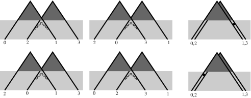
Figure 2: Terms in disk four-point amplitudes. The four figures on the left correspond to physically uninteresting processes and are discarded. The two on the right describe the terms which are reproduced from MQM analysis.

The physically interesting terms, Figure 2 right, are obtained from the recursion relations with the number of inhomogeneous terms reduced,

$$~{}\hskip-25.60747pt\frac{d(k_{1},s_{0},s_{1}^{\prime})}{d(k_{1}-\frac{ib}{2},s_{0},s_{1})}\left\langle{{}^{s_{3}}[U^{+}_{k_{0}}]^{s_{0}}[U^{+}_{k_{1}-\frac{ib}{2}}]^{s_{1}}[U^{+}_{k_{2}}]^{s_{2}}[U^{+}_{k_{3}}]^{s_{3}}}\right\rangle$$ (2.23)

$$~{}\hskip-34.1433pt+\frac{d(k_{2},s_{1},s_{2})}{d(k_{2}-\frac{ib}{2},s_{1}^{\prime},s_{2})}\left\langle{{}^{s_{3}}[U^{+}_{k_{0}}]^{s_{0}}[U^{+}_{k_{1}}]^{s_{1}^{\prime}}[U^{+}_{k_{2}-\frac{ib}{2}}]^{s_{2}}[U^{+}_{k_{0}}]^{s_{3}}}\right\rangle$$

$$= -\frac{8\pi^{3}\,\nu^{Q}\,b\,e^{-2\pi bk_{1}}}{e^{2\pi b(k_{3}+s_{1})}-e^{2\pi b(-k_{2}+s_{3})}}+\frac{8\pi^{3}\,\nu^{Q}\,b\,e^{2\pi bk_{2}}}{e^{2\pi b(k_{1}+s_{3})}-e^{2\pi b(-k_{0}+s_{1})}}$$

and a similar equation involving $i/2b$ shifts. We found that they are solved for $b=1$ by

$$\left\langle{{}^{s_{3}}[U^{-}_{k_{0}}]^{s_{0}}[U^{+}_{k_{1}}]^{s_{1}}[U^{-}_{k_{2}}]^{s_{2}}[U^{+}_{k_{3}}]^{s_{3}}}\right\rangle$$

$$= 16i\pi^{3}\nu^{2}e^{-2\pi k_{2}}\times\frac{d(k_{1},s_{0},s_{1})d(k_{3},s_{2},s_{3})-d(k_{0},s_{3},s_{0})^{-1}d(k_{2},s_{1},s_{2})^{-1}}{(e^{2\pi(k_{1}+s_{2})}-e^{2\pi(-k_{2}+s_{0})})(e^{2\pi(k_{3}+s_{1})}-e^{2\pi(-k_{2}+s_{3})})}$$

$$= 4i\pi^{3}\nu^{2}\,e^{-\pi(k_{1}+k_{3})}\times\frac{d(k_{1},s_{0},s_{1})d(k_{3},s_{2},s_{3})-d(k_{0},s_{3},s_{0})^{-1}d(k_{2},s_{1},s_{2})^{-1}}{\sinh\pi(k_{1}+k_{2}-s_{0}+s_{2})\sinh(k_{2}+k_{3}+s_{1}-s_{3})}.$$

A remarkable property of (LABEL:4ptsol2) is that it has a certain symmetry under the exchange of $k_{a}$ and $s_{a}$. To see this, let us introduce four positive “winding” parameters $y_{0},y_{1},y_{2},y_{3}$ such that

$$k_{0}=-(y_{3}+y_{0}),~{}~{}~{}k_{1}=y_{0}+y_{1},~{}~{}~{}k_{2}=-(y_{1}+y_{2}),~{}~{}~{}k_{3}=y_{2}+y_{3}.$$ (2.25)

Then the conservation of momenta is satisfied automatically. The parameters $y_{i}$ are determined up to a common translation

$$y_{0,2}\to y_{0,2}+a,\qquad y_{1,3}\to y_{1,3}-a\,.$$ (2.26)

By inserting them into (LABEL:4ptsol2) one finds that in Maldacena’s limit the non-trivial part of the amplitude depends only on the differences $\hat{y}_{i}=y_{i}-s_{i}$:

$$\left\langle{{}^{s_{3}}[U^{-}_{k_{0}}]^{s_{0}}[U^{+}_{k_{1}}]^{s_{1}}[U^{-}_{k_{2}}]^{s_{2}}[U^{+}_{k_{3}}]^{s_{3}}}\right\rangle = 4\pi^{3}\,\nu^{2}\,\prod_{j=0}^{3}e^{-2\pi is_{j}^{2}-\pi(s_{j}+y_{j})}$$ (2.27)

$$\hskip-82.51282pt\times\ \frac{e^{if(-\pi\hat{y}_{0}+\pi\hat{y}_{1})+if(-\pi\hat{y}_{2}-\pi\hat{y}_{3})}-e^{-if(\pi\hat{y}_{3}-\pi\hat{y}_{0})+if(-\pi\hat{y}_{1}-\pi\hat{y}_{2})}}{\sinh\pi(\hat{y}_{2}-\hat{y}_{0})\ \sinh\pi(\hat{y}_{1}-\hat{y}_{3})}.$$

In other words, the four-point amplitude is almost symmetric under $s_{i}-L\leftrightarrow L-y_{i}$. The change of sign can be understand as follows: increasing the energy makes the tip of the folded string go further while increasing the boundary parameter has the opposite effect. The parameter $y$ is in some loose sense T-dual to the original time variable; such a duality transformation is discussed for the AdS disk amplitudes in [27].

3 Long folded strings in Matrix Quantum Mechanics

3.1 Asymptotic states and chiral formalism of MQM

The dual matrix description of the 2D string theory in the linear dilaton background is given by a dimensional reduction of a 2D YM theory to one dimension, known also as Matrix Quantum Mechanics [12]. The theory involves one gauge field ${\bf A}=\{A_{i}^{j}\}$ and one scalar field ${\bf X}=\{X_{i}^{j}\}$, both hermitian $N\times N$ matrices. It is formally defined by the action

$${\cal S}=\int dt\,{\rm tr\,}\left[{\bf P}\,\nabla_{\bf A}{\bf X}-{\textstyle{\frac{1}{2}}}({\bf P}^{2}-{\bf X}^{2})\right],$$ (3.1)

where $\nabla_{\bf A}{\bf X}=\partial_{t}{\bf X}-i[{\bf A},{\bf X}]$ is the covariant time derivative. The action (3.1) can be considered as an effective action describing the states near a local maximum of a confining potential for the scalar field. In this approximation a generic potential can be replaced by inverse gaussian potential and a large cutoff parameter $\Lambda$. The number of colors $N$ should be tuned appropriately with the cutoff $\Lambda$ before taking the large $N$ limit.

The Hilbert space of MQM decomposes as a direct sum

$$\mathcal{H}=\mathcal{H}_{0}+\sum_{n=1}^{\infty}\mathcal{H}_{n}\,,$$ (3.2)

where $\mathcal{H}_{0}$ is the singlet sector and the sector $\mathcal{H}_{n}$ is obtained by adding $n$ Wilson lines in the adjoint representation. The sector $\mathcal{H}_{n}$ can be further decomposed into a direct sum of irreducible representations of $U(N)$ whose Young tableaux contain $n$ boxes and $n$ ‘antiboxes’. The Young tableaux for the allowed representations wih $n=1,2$ are represented in Fig. 3.

In the singlet sector, $n=0$, the action (3.1) describes a system of $N$ non-relativistic free fermions in the upside-down quadratic potential [12]. The ground state of the system is characterized by the Fermi level $E_{F}=-\mu$. The cutoff $\Lambda$ then gives the energy (with minus sign) of the $N$-th level below the surface of the fermi sea. In the large $N$ limit, the non-singlet sectors can be described in terms of impurities in the fermi sea. The non-singlet excitations of MQM have been studied in [28, 29, 3]. Let ${\cal D}$ be an allowed irreducible representation of $SU(N)$. Then the radial part of the Hamiltonian contains a term with Calogero type interaction between the eigenvalues,

$$H^{({\cal D})}=-\frac{1}{2}\sum_{j=1}^{N}\left({\partial^{2}\over\partial x_{j}^{2}}+x_{j}^{2}\right)+\frac{1}{2}\sum_{j\neq k}^{N}\frac{{\cal D}(E_{j}^{k}){\cal D}(E_{k}^{j})}{(x_{j}-x_{k})^{2}}\,.$$ (3.3)

where ${\cal D}(E_{j}^{k})$ is a realization of the $N\times N$ matrix $(E_{j}^{k})_{l}^{m}=\delta_{j}^{m}\delta_{l}^{k}$.

In the adjoint representation, $n=1$, the wave function is an $N\times N$ traceless matrix. By an $SU(N)$ rotation it can be diagonalized as

$$\Psi_{i}^{j}(\mathbf{X})=\delta_{i}^{j}\ \psi_{i}(\mathbf{X}),$$

with $\sum_{i}\psi_{i}=0$. Then the radial part of the Schrödinger equation closes on the components $\psi_{1},\dots,\psi_{N}$:

$$H^{\rm adj}\psi_{i}=-\sum_{j=1}^{N}{{\textstyle{\frac{1}{2}}}}(\partial_{i}^{2}+x_{i}^{2})\psi_{i}+\sum_{j(\not=i)}^{N}{(\psi_{i}-\psi_{j})\over(x_{i}-x_{j})^{2}}\,.$$ (3.4)

The solution of this equation in the large $N$ limit  gives the wavefunction of one quasiparticle.

Once we know the solution of the wave equation in the adjoint, which was found in [17], we can try to explore the higher sectors. To the leading order in $1/\mu$, the sector $\mathcal{H}_{n}$ describes $n$ non-interacting quasiparticles. The statistics of the quasiparticles is determined by choice of the irreducible representation. Our analysis of the Calogero type wave equation (see Appendix E) shows that the Hamiltonian indeed decomposes into a sum of terms (3.4) associated with the $n$ quasiparticles, and a two-body interaction Hamiltonian, which is of order $1/\mu$.

Instead of trying to solve the wave equation, in this paper we will follow an alternative approach, the chiral quantization of MQM [4], which proved to be very efficient in the singlet sector. Since the potential is unbounded, any observable can be formulated in terms of scattering amplitudes between asymptotic states that characterize the system at the infinite past and in the infinite future. Usually the scattering matrix relating the incoming and the outgoing asymptotic states is extracted from the asymptotics of the solution of the Schrödinger equation. In the case of quadratic potential it happens that the $S$-matrix can be constructed directly, without passing through the evaluation of the wave function. This is possible due to the important property of the MQM that the asymptotic in- and out-states depend on the light cone variables

$$\mathbf{X}_{{}_{+}}=\frac{{\bf X}+{\bf P}}{\sqrt{2}},\ \ \ \ \quad X_{-}=\frac{{\bf X}-{\bf P}}{\sqrt{2}}.$$ (3.5)

For example, the operators

$$T^{+}_{E}={\rm tr\,}\,\mathbf{X}_{{}_{+}}^{iE},\qquad T^{-}_{E}={\rm tr\,}\,\mathbf{X}_{{}_{-}}^{-iE}.$$ (3.6)

describe the left- and right-moving tachyons with energy $E$ [30]. The time evolution of the asymptotic states is governed by the Hamiltonian

$$H=-\frac{1}{2}{\rm tr\,}(\mathbf{X}_{{}_{+}}\mathbf{X}_{{}_{-}}+\mathbf{X}_{{}_{-}}\mathbf{X}_{{}_{+}})\,,$$ (3.7)

and the general solution of the corresponding Schrödinger equation is

$$\Phi^{\pm}(\mathbf{X}_{{}_{\pm}},t)=e^{\mp{1\over 2}N^{2}t}\ \Phi^{\pm}(e^{\mp t}\mathbf{X}_{{}_{\pm}}).$$ (3.8)

Thus any homogeneous function is an eigenstate of the Hamiltonian (3.7).

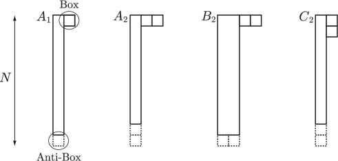
Figure 3: The lowest representations allowed in MQM.

The outgoing and the incoming states are related by matrix Fourier transformation

$$\Phi^{+}(\mathbf{X}_{{}_{+}}) =\ \int d\mathbf{X}_{{}_{-}}e^{-i{\rm tr\,}\,\mathbf{X}_{{}_{+}}\mathbf{X}_{{}_{-}}}\,\Phi^{-}(\mathbf{X}_{{}_{-}})\,,$$ (3.9)

which represents the scattering operator in the chiral basis.

The wave functions in the sector $\mathcal{H}_{n}$ transform according to the $n$-th power of the adjoint representation,

$$\Phi^{\pm}(\Omega\mathbf{X}_{{}_{\pm}}\Omega^{\dagger})={\rm Ad}(\Omega)^{\otimes n}\,\Phi^{\pm}(\mathbf{X}_{{}_{\pm}}),\qquad\Omega\in SU(N).$$ (3.10)

For any $n$, ${\rm Ad}(\Omega)^{\otimes n}$ decomposes into a direct sum of irreducible representations. The projection to any given irreducible representation is obtained by applying the corresponding Young symmetrizer. The scattering amplitude between the states $\Phi^{-}$ and $\Phi^{+}$ is given by the inner product

$$\left(\Phi^{+},\Phi^{-}\right)=\int d\mathbf{X}_{{}_{+}}d\mathbf{X}_{{}_{-}}\ e^{i{\rm tr\,}\,\mathbf{X}_{{}_{+}}\mathbf{X}_{{}_{-}}}\ {\rm tr\,}^{{}_{\!\!(n)}}\,\overline{\Phi^{+}(\mathbf{X}_{{}_{+}})}\Phi^{-}(\mathbf{X}_{{}_{-}})\,,$$ (3.11)

where ${\rm tr\,}^{{}_{\!\!(n)}}$ denotes the trace in the $n$-th tensor product.

With this description of the non-singlet sectors we can represent any state as a polynomial of the matrix fields $\mathbf{X}_{{}_{+}}$ or $\mathbf{X}_{{}_{-}}$ multiplying a singlet wave function. Below we will see that similarly to the closed strings, the long folded strings are represented in MQM by creation and annihilation operators made of the matrix elements of $\mathbf{X}_{{}_{+}}$ and $\mathbf{X}_{{}_{-}}$. Thus the eigenfunction representing a state with $n$ folded strings and $m$ tachyons is

$$[\Phi^{\pm}(E_{1},...,E_{n};E^{\prime}_{1},...,E^{\prime}_{m})]_{j_{1},...,j_{n}}^{l_{1},...,l_{n}}=\prod_{a=1}^{n}[\mathbf{X}_{{}_{\pm}}^{\pm iE^{\pm}_{a}}]_{{}_{j_{a}}}^{{}^{l_{a}}}\ \prod_{b=1}^{m}{\rm tr\,}\mathbf{X}_{{}_{\pm}}^{\pm iE^{\prime}_{b}}\ \ \Phi_{0}^{\pm}(\mathbf{X}_{{}_{\pm}})\,,$$ (3.12)

where $\Phi_{0}^{\pm}$ is the ground state wave function.

The scattering amplitude for such states is given by the inner product of an incoming and an outgoing state of the form (3.12) divided by the inner product of the left and right ground states. It is therefore useful to introduce for each pair of functions $F^{+}(\mathbf{X}_{{}_{-}}),F^{-}(\mathbf{X}_{{}_{+}})$ the expectation value

$$\left\langle\,\!\mu\left|\,F^{+}F^{-}\,\right|\mu\!\,\right\rangle:={\left(\Phi_{0}^{+}F^{+},F^{-}\Phi^{-}_{0}\right)\over\left(\Phi^{+}_{0},\Phi_{0}^{-}\right)}.$$ (3.13)

In this way all observables in the non-singlet sector of MQM can be obtained as multi trace correlators of an effective two-matrix model with non-confining potential ${\rm tr\,}\mathbf{X}_{{}_{+}}\mathbf{X}_{{}_{-}}$. The observables in this “non-compact” matrix model can be evaluated by an appropriate regularization. It happens that some of the results obtained for the usual, “compact” matrix models, can be applied here.

The $U(N)$ symmetry allows to reduce the original $N^{2}$ degrees of freedom to the $N$ eigenvalues $x^{\pm}_{1}\dots x^{\pm}_{N}$ of the matrices $\mathbf{X}_{{}_{+}}$ or $\mathbf{X}_{{}_{-}}$. The evaluation of the scattering amplitude is achieved in two steps [18]. The first step consists in integrating out the angular degrees of freedom in the matrix integration measure

$$d\mathbf{X}_{{}_{\pm}}=d\Omega_{\pm}\,dx^{\pm}_{1}\dots dx^{\pm}_{N}\,\Delta^{2}(x_{\pm}),$$ (3.14)

where $\Delta(x_{\pm})=\prod_{i<j}(x^{\pm}_{i}-x^{\pm}_{j})$ is the Vandermonde determinant. The angular integral in the inner product (3.11) is then of the form

$$I_{n}(\mathbf{X}_{{}_{+}},\mathbf{X}_{{}_{-}})=\int\limits_{SU(N)}\!\!\!d\Omega\ {\rm Ad}(\Omega)^{\otimes n}\ e^{i\mathbf{X}_{{}_{+}}\Omega\mathbf{X}_{{}_{-}}\Omega^{\dagger}}.$$ (3.15)

The second step is to take the large $N$ limit and express the result in terms of the collective field, the phase space eigenvalue density $\rho(x^{+},x^{-})$. In the well studied singlet sector, $n=0$, the integral (3.15) is the Harish-Chandra-Itzykson-Zuber integral [32]. In this simplest case the transition amplitudes

$$S(E^{+}_{1},...,E_{m}^{+};E^{-}_{1},...,E^{-}_{n})=\langle\mu|\prod_{a=1}^{m}{\rm tr\,}\mathbf{X}_{{}_{+}}^{iE^{+}_{a}}\ \prod_{b=1}^{n}{\rm tr\,}\mathbf{X}_{{}_{-}}^{iE^{-}_{b}}|\mu\rangle$$

then can be formulated in terms of the scalar product in the fermi sea vacuum [4]. In the general case the integral (3.15) was evaluated by Shatashvili [33]. In the case $n=1$ a formula suitable for taking the large $N$ limit was guessed by Morozov [34] and proved later by Eynard and collaborators [35, 19]. More general integrals and and other gauge groups were studied in [36, 37]. Taking the large $N$ expansion of these exact results is a delicate task. In this aspect, the paper [20] proved to be very useful for our problem.

3.2 The reflection amplitude in the adjoint sector $(n=1)$

The sector with $n=1$ contains only one non-trivial representation, the adjoint. One can think of this sector as the fermi sea in presence of an impurity, or quasiparticle. In terms of the string theory, the adjoint sector describes incoming and outgoing asymptotic states containing one folded string. In absence of tachyons the inner product in this sector gives the reflection amplitude of the quasiparticle associated with the tip of the folded string [18]. In the compactified Euclidean theory this sector describes states with one vortex and one anti-vortex. The eigenfunction describing a folded string with energy $E$ is of the form

$$[\Phi^{\pm}(E)]_{j}^{l}=\left([\mathbf{X}_{{}_{\pm}}^{\pm iE}]_{{}_{j}}^{{}^{l}}-\frac{1}{N}\mbox{tr}(\mathbf{X}_{{}_{\pm}}^{\pm iE})\delta_{{}_{j}}^{{}^{l}}\right)\Phi_{0}^{\pm}(\mathbf{X}_{{}_{\pm}}),$$ (3.16)

where $\Phi_{0}^{\pm}$ is the ground state wave function. To the leading order in the large $N$ limit one can replace $SU(N)$ by $U(N)$ and neglect the term subtracting the trace. More general wave functions,

$$[\mathbf{X}_{{}_{\pm}}^{\pm iE}]_{{}_{j}}^{{l}}\ {\rm tr\,}\mathbf{X}_{{}_{\pm}}^{\pm iE_{1}}{\rm tr\,}\mathbf{X}_{{}_{\pm}}^{\pm iE_{2}}\cdots{\rm tr\,}\mathbf{X}_{{}_{\pm}}^{\pm iE_{m}}\ \Phi_{0}^{\pm}(\mathbf{X}_{{}_{\pm}})\,,$$

describe a folded string in presence of $m$ tachyons. We will focus on the states of the form (3.16). For such states the scattering matrix reduces to the reflection factor for one adjoint particle, which is given by the normalized inner product

$$R_{1}(E_{+},E_{-})=\left\langle\,\!\mu\left|\,{\rm tr\,}(\mathbf{X}_{{}_{+}}^{iE_{+}}\mathbf{X}_{{}_{-}}^{iE_{-}})\,\right|\mu\!\,\right\rangle\,.$$ (3.17)

Evaluating the integral over the angles by the Morozov-Eynard formula, we obtain an expression depending only on the eigenvalues of the matrices $\mathbf{X}_{{}_{+}}$ and $\mathbf{X}_{{}_{-}}$. In the large $N$ limit the result can be expressed in terms of the joint eigenvalue density $\rho(x^{{}^{+}},x^{{}^{-}})$ for the ground state. The Morozov-Eynard formula takes most simple form [19] when expressed in terms of the resolvents

$$W\!_{\!{}_{\pm}}(\xi^{{}_{\pm}}):={1\over\xi^{{}_{\pm}}+{\bf X}_{\pm}}\,.$$ (3.18)

The operators creating eigenstates with given energy (3.16) are related to the operators (3.18) by the integral transformation

$${\bf X}^{-iE}={i\over\pi}\sinh\pi E\int\limits_{0}^{\infty}{d\xi\over\xi+{\bf X}}\,\,\xi^{-iE}\,.$$ (3.19)

The inverse transformation is

$${1\over\xi+{\bf X}}=-{i\over 2\xi}\int\limits_{C}{dE\over\sinh\pi E}\ \xi^{iE}\,{\bf X}^{-iE}\,,$$ (3.20)

where the integration contour $C$ is parallel to the real axes and passing between the poles at $E=0$ and $E=i$ of the integrand. It is most natural to choose $C={\mathbb{R}}+{\textstyle{\frac{1}{2}}}i$, which we will do in the following.

We therefore first evaluate the normalized inner product for the resolvents (3.18),

$$G_{1}(\xi^{{}_{+}},\xi^{{}_{-}}):=\left\langle\,\!\mu\left|\,{\rm tr\,}[W\!_{\!{}_{+}}(\xi^{{}_{+}})W\!_{\!{}_{-}}(\xi^{{}_{-}})]\,\right|\mu\!\,\right\rangle\,,$$ (3.21)

and then apply the integral transformation (3.19) to obtain the reflection amplitude in the $E$-space. The expectation value (3.21) is the basic single-trace mixed correlator in the effective two-matrix model we mentioned before. The result, obtained in [18], is surprisingly simple:

$$G_{1}(\xi^{{}_{+}},\xi^{{}_{-}}) = e^{-iS(\xi^{{}_{+}},\xi^{{}_{-}})}\,,$$

$$S(\xi^{{}_{+}}.\xi^{{}_{-}}) = \int{dx^{{}^{+}}dx^{{}^{-}}\over 2\pi}\ {\rho(x^{{}^{+}},x^{{}^{-}})\over(\xi^{{}_{+}}+x^{{}^{+}})(\xi^{{}_{-}}+x^{{}^{-}})}\,,$$ (3.22)

where $\rho(x^{{}^{+}},x^{{}^{-}})$ is the semiclassical eigenvalue density of the fermionic liquid.

This integral is logarithmically divergent and needs a regularization. We introduce a cutoff ${\tilde{\Lambda}}\gg\mu$ as the depth of the Fermi sea explored by the average. We assume that ${\tilde{\Lambda}}\ll\Lambda$, so that we still can use the spectral density for the upside-down harmonic oscillator. The part of the Fermi sea that corresponds to the interval of energies $-\mu<E<-{\tilde{\Lambda}}$ is described by the density function

$$\rho(x^{{}^{+}},x^{{}^{-}})=\theta(x^{{}^{+}}x^{{}^{-}}-\mu)\,\theta({\tilde{\Lambda}}-x^{{}^{+}}x^{{}^{-}}).$$ (3.23)

The result of the integration with this density depends only on the product $\xi^{{}_{+}}\xi^{{}_{-}}$:

$$S(\xi^{{}_{+}},\xi^{{}_{-}})=f\left(T-t\right)-f\left(-t\right)\,,$$ (3.24)

where we denoted

$$T={1\over 2}\log{{\tilde{\Lambda}}\over\mu},\qquad t={1\over 2}\log{\xi^{{}_{+}}\xi^{{}_{-}}\over\mu}$$ (3.25)

and the function $f$ is the same as in (2.11). Applying the integral transformation (3.19) to both arguments of ${G_{1}}(\xi^{{}_{+}},\xi^{{}_{-}})$, we get

$$R_{1}({E}_{+},{E}_{-})=-\frac{\sinh(\pi{E}_{+})\sinh(\pi{E}_{-})}{\pi^{2}}\int_{0}^{\infty}d\xi^{{}_{+}}d\xi^{{}_{-}}(\xi^{{}_{+}})^{i{E}_{+}}(\xi^{{}_{-}})^{i{E}_{-}}\ G_{1}(\xi^{{}_{+}},\xi^{{}_{-}}).$$ (3.26)

At this point we change the variables as $\xi^{\pm}=\sqrt{\mu}\,e^{t\pm\tau}\,.$ The integral over $\tau$ produces a delta function imposing the energy conservation,

$$R_{1}({E}_{+},{E}_{-})={\cal R}_{1}({E}_{+})\ \delta({E}_{+}-{E}_{-})\,.$$ (3.27)

The reflection factor for one quasiparticle is given by the remaining integral in $t$:

$${\cal R}_{1}({E})=-{2\over\pi}\sinh^{2}\!\pi E\,\,\mu^{-i{E}+1}\,\int_{-\infty}^{\infty}dt\,e^{2t(-i{E}+1)-if(T-t)+if(-t)}\,.$$ (3.28)

In the limit $T\to\infty$ we can use the approximation $f(T-t)=(T-t)^{2}/\pi$ and then write the exponent, using (A.24), as $2t-if(t)-2i(E-T/\pi)t+i\pi/6$. The integral is evaluated using the last equation (A.14). The final result for the reflection factor is

$${\cal R}_{1}({E})=2\Lambda\,e^{-i\alpha}\sinh^{2}\!\pi E\,\mu^{-iE}\,e^{-iT^{2}/\pi}e^{-2E\pi+if(T-\pi E)}\,\,.$$ (3.29)

We see that the reflection factor depends on the shifted energy $\hat{\epsilon}=E-T/\pi$, where the constant $T={1\over 2}\log{\tilde{\Lambda}}/\mu$ is in fact the logarithmic energy gap between the singlet and the adjoint sector discovered in [28]. We therefore subtract, as in [1], this constant from the energy and introduce the shifted energy variables

$$\epsilon=E-{1\over 2\pi}\ln{\tilde{\Lambda}},\qquad\hat{\epsilon}=\epsilon+{1\over 2\pi}\ln{\mu}={E}-T/\pi\,,$$ (3.30)

where $\hat{\epsilon}$ is assumed finite. Then we can approximate $\sinh\pi E\approx{1\over 2}e^{\pi E}$ and the scattering phase takes the form

$${\cal R}_{1}({E}) = \ {\textstyle{\frac{1}{2}}}\Lambda\,e^{-i\alpha}\,\mu^{-i{E}}\ e^{-iT^{2}/\pi}e^{if(-\pi\hat{\epsilon})}$$ (3.31)

$$= -{\textstyle{\frac{1}{2}}}{\tilde{\Lambda}}\,e^{-i\pi/4}e^{-i\log^{2}{{\tilde{\Lambda}}}/4\pi}\times e^{i\pi\epsilon^{2}-if(\pi\hat{\epsilon})}\,.$$ (3.33)

Let us compare this expression with the two-point function in the worldsheet theory with $s=s^{\prime}=M$ and $k\sim M$,

$$\left\langle\,U^{+}_{k}U^{-}_{-k}\,\right\rangle={\pi\nu^{2}\over\sinh 2\pi|k|}d(|k|)=\pi^{2}\nu^{2}\,2e^{-2\pi k}e^{-i\pi/4}e^{-4\pi iM^{2}}e^{if(2\pi M-\pi k)}\,.$$ (3.34)

Remarkably, the two expressions coincide (up to a constant phase, which can be absorbed in the normalization of the wave functions) upon the identification

$$k=E,\qquad s=s^{\prime}={T/2\pi},\qquad\nu^{2}=\pi\mu\,.$$ (3.35)

Therefore the cutoff ${\tilde{\Lambda}}$, the depth of the fermi sea felt by the collective excitation, is related to the boundary cosmological constant in the worlsheet theory:

$${\tilde{\Lambda}}=\mu_{{}_{B}}^{2}\,.$$ (3.36)

The remaining factor can be absorbed into the normalization of the boundary operators $U^{\pm}_{\pm k}$.

Note that the reflection factor (3.33) is given, up to a complex conjugation and a numerical factor, by the same function as the mixed correlator (3.21 ):

$${\cal R}_{1}(E)={\tilde{\Lambda}}^{1-iE}\ \overline{G_{1}(\xi^{{}_{+}},\xi^{{}_{-}})}\qquad\xi^{{}_{+}}\xi^{{}_{-}}={\tilde{\Lambda}}\,e^{-\pi E}=\mu\,e^{-\pi\hat{\epsilon}}\,.$$ (3.37)

3.3 The reflection amplitude in the sector $n=2$

Now we will evaluate the reflection amplitudes for the states (3.12) with $n=2$, in the leading and in the subleading order. The scattering matrix is not diagonal for such states. It gets diagonalized in the basis of the irreducible representations with $n=2$, which we describe below.

In the sector $\mathcal{H}_{2}$ there are four irreducible representations (denoted as $A_{2},\bar{A}_{2},B_{2}$ and $C_{2}$ in [29]). Their Young tableaux are shown in Fig. 3. For general $n$, the representations $B_{n}$ and $C_{n}$ are defined by tensors with $n$ upper and $n$ lower indices, respectively totally symmetric and totally antisymmetric under permutations of the upper and lower indices, associated with boxes and antiboxes. The representations $A_{n}$ are totally symmetric in boxes and totally antisymmetric in antiboxes, and similarly for $\bar{A}_{n}$. The zero weight states in the sector with $n=2$ are of the form

$$\Psi_{ik}^{jl}=P_{ik}^{jl}\ \psi_{ik}\,,$$

where $P_{ik}^{jl}$ is a standard tensor associated with the corresponding Young symmetrizer. In the four irreducible representations, $A_{2},\bar{A}_{2},B_{2}$ and $C_{2}$, it is given respectively by $\delta_{[i}^{\{j}\delta_{k]}^{l\}},\delta_{\{i}^{[j}\delta_{k\}}^{l]},\delta_{\{i}^{\{j}\delta_{k\}}^{l\}}$ and $\delta_{[i}^{[j}\delta_{k]}^{l]}$, where $[\cdot,\cdot]$ denotes antisymmetrization and $\{\cdot,\cdot\}$ denotes symmetrization. In order to extract the irreducible part, one needs further to impose the tracelessness condition for any pair of upper and lower indices, but this can be skipped in the two leading orders in the large $N$ limit.

Now let us return to the states (3.12) with $n=2$. As in the case $n=1$, it is advantageous first to evaluate the inner product of the wave functions in the coordinate space

$$\tilde{\Phi}_{{}_{j_{1},j_{2};k_{1},k_{2}}}^{\pm}(\xi^{{}_{\pm}}_{1},\xi^{{}_{\pm}}_{2})=[W\!_{\!{}_{\pm}}(\xi^{{}_{\pm}}_{1})]_{{}_{j_{1}}}^{{}^{k_{1}}}[W\!_{\!{}_{\pm}}(\xi^{{}_{\pm}}_{2})]_{{}_{j_{2}k_{2}}}\,\Phi^{\pm}_{0}\,.$$ (3.38)

The inner product is expressed in terms of mixed two-trace correlator

$$G_{1,1}(\xi^{{}_{+}}_{1},\xi^{{}_{-}}_{1};\xi^{{}_{+}}_{2},\xi^{{}_{-}}_{2})=\left\langle\,\!\mu\left|\,{\rm tr\,}[W_{+}(\xi^{{}_{+}}_{1})W_{-}(\xi^{{}_{-}}_{1})]\ {\rm tr\,}[W_{+}(\xi^{{}_{+}}_{2})W_{-}(\xi^{{}_{-}}_{2})]\,\right|\mu\!\,\right\rangle$$

and the mixed one-trace correlator

$$G_{2}(\xi^{{}_{+}}_{1},\xi^{{}_{-}}_{1},\xi^{{}_{+}}_{2},\xi^{{}_{-}}_{2})=\left\langle\,\!\mu\left|\,{\rm tr\,}[W_{+}(\xi^{{}_{+}}_{1})W_{-}(\xi^{{}_{-}}_{1})W_{+}(\xi^{{}_{+}}_{2})W_{-}(\xi^{{}_{-}}_{2})]\,\right|\mu\!\,\right\rangle\,.$$

The projections to the four irreps in the sector $n=2$ are obtained by (anti)symmetrization:

$$\langle\mu|\tilde{\Phi}^{+}\ \tilde{\Phi}^{-}|\mu\rangle_{A_{2}} = G_{1,1}(\xi^{{}_{+}}_{1},\xi^{{}_{-}}_{1};\xi^{{}_{+}}_{2},\xi^{{}_{-}}_{2})-\{\xi^{{}_{-}}_{1}\leftrightarrow\xi^{{}_{-}}_{2}\}\ =\ \langle\mu|\tilde{\Phi}^{+}\ \tilde{\Phi}^{-}|\mu\rangle_{\bar{A}_{2}}$$

$$\langle\mu|\tilde{\Phi}^{+}\ \tilde{\Phi}^{-}|\mu\rangle_{B_{2}} = G_{1,1}(\xi^{{}_{+}}_{1},\xi^{{}_{-}}_{1};\xi^{{}_{+}}_{2},\xi^{{}_{-}}_{2})+G_{2}(\xi^{{}_{+}}_{1},\xi^{{}_{-}}_{1},\xi^{{}_{+}}_{2},\xi^{{}_{-}}_{2})+\{\xi^{{}_{-}}_{1}\leftrightarrow\xi^{{}_{-}}_{2}\}\,,$$

$$\langle\mu|\tilde{\Phi}^{+}\ \tilde{\Phi}^{-}|\mu\rangle_{C_{2}} = G_{1,1}(\xi^{{}_{+}}_{1},\xi^{{}_{-}}_{1};\xi^{{}_{+}}_{2},\xi^{{}_{-}}_{2})-G_{2}(\xi^{{}_{+}}_{1},\xi^{{}_{-}}_{1},\xi^{{}_{+}}_{2},\xi^{{}_{-}}_{2})+\{\xi^{{}_{-}}_{1}\leftrightarrow\xi^{{}_{-}}_{2}\}\,.$$ (3.39)

Each term on the r.h.s. can be expanded in $1/\mu$. To the leading order $\mu^{2}$ only the first term contributes, where it factorizes to

$$G_{1,1}(\xi^{{}_{+}}_{1},\xi^{{}_{-}}_{1};\xi^{{}_{+}}_{2},\xi^{{}_{-}}_{2})=G_{1}(\xi^{{}_{+}}_{1},\xi^{{}_{-}}_{1})\,G_{1}(\xi^{{}_{+}}_{2},\xi^{{}_{-}}_{2})\,+O(\mu^{0}).$$

The integral transformation (3.19) gives

$$R_{2}^{(0)}(E_{1}^{+},E_{2}^{+},E_{1}^{-},E_{2}^{-})=\delta(E_{1}^{+}-E_{1}^{-})\,\delta(E_{2}^{+}-E_{2}^{-}){\cal R}_{1}(E_{1}^{+})\,{\cal R}_{1}(E_{2}^{+})\,.$$ (3.40)

To this order the inner product are given by the (anti)symmetrized product of two expectation values (3.21), associated with each trace. This is the approximation of dilute gas of quasiparticles.

The subleading term is given by $G_{2}(\xi_{1}^{+},\xi_{2}^{+},\xi_{1}^{-},\xi_{2}^{-})$. Here we will focus on this amplitude and leave the next order $\mu^{0}$, which is given by the connected correlator of the product of two traces, for future work. The mixed one-trace correlators $G_{n}$ in the effective two-matrix model can be expressed through the lowest one-trace correlator $G_{1}$ by the general formula derived in [20]. In the case $n=2$ it states

$$G_{2}(\xi_{1}^{+},\xi_{2}^{+},\xi_{1}^{-},\xi_{2}^{-}) = i\,{G_{1}(\xi_{1}^{+},\xi_{1}^{-})G_{1}(\xi_{2}^{+},\xi_{2}^{-})-G_{1}(\xi_{1}^{+},\xi_{2}^{-})G_{1}(\xi_{2}^{+},\xi_{1}^{-})\over(\xi_{1}^{+}-\xi_{2}^{+})(\xi_{1}^{-}-\xi_{2}^{-})}\,.$$ (3.41)

A simpler derivation of this formula, due to L. Cantini, can be found in Orantin’s thesis [38]. The advantage of this derivation, which we give in Appendix C, is that it can be applied also for our non-compact effective two-matrix model.

The next step is to perform the integral transformation (3.19) to each of the arguments. The calculation, this time non-trivial, is presented in Appendix B. The result contains a $\delta$-function for the energy conservation, so we define the subleading $n=2$ reflection amplitude ${\cal R}_{2}$ by

$$R_{2}^{(1)}(E_{1}^{+},E_{2}^{+},E_{1}^{-},E_{2}^{-})=\delta(E_{1}^{+}+E_{2}^{+}-E_{1}^{-}-E_{2}^{-})\ {\cal R}_{2}(E_{1}^{+},E_{2}^{+};E_{1}^{-},E_{2}^{-})\,.$$ (3.42)

For energies $E_{j}^{\pm}=\epsilon_{j}^{\pm}+{1\over 2\pi}\ln{\tilde{\Lambda}}$, with $\epsilon_{j}^{\pm}$ finite,

$${\cal R}_{2}(E_{1}^{+},E_{2}^{+},E_{1}^{-},E_{2}^{-}) = -{2\over{\tilde{\Lambda}}}\ \epsilon^{\pi(E_{1}^{+}+E_{2}^{+})}\ {{\cal R}_{1}(E_{1}^{+}){\cal R}_{1}(E_{2}^{+})-{\cal R}_{1}(E_{1}^{-}){\cal R}_{1}(E_{2}^{-})\over\sinh\pi(E^{+}_{1}-E^{-}_{1})\sinh\pi(E^{+}_{1}-E^{-}_{2})}$$ (3.43)

$$= -\frac{2}{\mu}\ e^{\pi(\hat{\epsilon}^{+}_{1}+\hat{\epsilon}^{+}_{2})}\ \frac{{{\cal R}_{1}}({E}_{1}^{+}){{\cal R}_{1}}({E}_{2}^{+})-{{\cal R}_{1}}({E}_{1}^{-}){{\cal R}_{1}}({E}_{2}^{-})}{\sinh{\pi(\hat{\epsilon}_{1}^{+}-\hat{\epsilon}_{1}^{-})}\sinh{\pi(\hat{\epsilon}_{1}^{+}-\hat{\epsilon}_{2}^{-})}}\,.$$ (3.46)

The $n=2$ reflection amplitude, given in the first two orders by (3.40) and (3.42), obviously satisfies the unitarity condition

$${\cal R}_{1}(E_{1}^{+}){\cal R}_{1}(E_{2}^{+})\,\overline{{\cal R}_{2}(E_{1}^{-},E_{2}^{-},E_{1}^{+},E_{2}^{+})}={\cal R}_{2}(E_{1}^{+},E_{2}^{+};E_{1}^{-},E_{2}^{-})\,\overline{{\cal R}_{1}(E_{1}^{-}){\cal R}_{1}(E_{2}^{-})}.$$ (3.47)

Let us compare the subleading reflection amplitude (3.43) with the 4-point disk amplitude in the Maldacena limit (LABEL:4ptsol2), evaluated in the worldsheet theory. If we identify

$$k_{0}=-E^{-}_{1},\quad k_{1}=E^{+}_{1},\quad k_{2}=-E^{-}_{2},\quad k_{3}=E^{+}_{2},$$ (3.48)

$$\quad s_{0}=s_{1}=s_{2}=s_{3}={T/2\pi},\quad\nu^{2}=\pi\mu\,,$$ (3.49)

then the two amplitudes are indeed equal to each other, up to a factor of 2. This factor can be absorbed in the normalization of the functional measure in the worldsheet calculation. After fixing the normalization of the boundary operators and the functional measure, there are no more ambiguities left.

If we express the energies in terms of the shifted winding parameters $y_{i}$ defined by (2.25),

$$E_{1}^{-}=y_{3}+y_{0},\quad E_{1}^{+}=y_{0}+y_{1},\quad E_{2}^{-}=y_{1}+y_{2},\quad E_{2}^{+}=y_{2}+y_{3}\,,$$ (3.50)

then we observe that the reflection amplitude in the $E$-space has again the same functional form as in the $\xi$-space,

$$\mathcal{R}_{2}(E_{1}^{+},E_{1}^{-},E_{2}^{+},E_{2}^{-})=-2i{\tilde{\Lambda}}^{2-i(E_{1}^{+}+E_{2}^{+})}\ \overline{G_{2}(\xi^{{}_{+}}_{1},\xi^{{}_{-}}_{1},\xi^{{}_{+}}_{2},\xi^{{}_{-}}_{2})}\,$$ (3.51)

with

$$\xi^{{}_{-}}_{1}={{\tilde{\Lambda}}^{1/2}}\,e^{-{1\over 2}\pi y_{0}},\quad\xi^{{}_{+}}_{1}={{\tilde{\Lambda}}^{1/2}}\,e^{-{1\over 2}\pi y_{1}},$$ (3.52)

(3.53)

$$\xi^{{}_{-}}_{2}={{\tilde{\Lambda}}^{1/2}}\,e^{-{1\over 2}\pi y_{2}},\quad\xi^{{}_{+}}_{2}={{\tilde{\Lambda}}^{1/2}}\,e^{-{1\over 2}\pi y_{3}}\,.$$ (3.54)

3.4 The reflection amplitude for $n>2$

Using the loop equations for the two-matrix model one can evaluate all mixed one-trace correlators

$${G}_{n}(\xi^{{}_{+}}_{1},\xi^{{}_{-}}_{1},\dots,\xi^{{}_{+}}_{n},\xi^{{}_{-}}_{n}):=\langle\mu|{\rm tr\,}\left[W_{+}(\xi^{{}_{+}}_{1})W_{-}(\xi^{{}_{-}}_{1})\dots W_{+}(\xi^{{}_{+}}_{k})W_{-}(\xi^{{}_{-}}_{n})\right]|\mu\rangle.$$

These correlators satisfy the recurrence equations found in [20], see Appendix C. The unique solution of the recurrence equations is given by the “Bethe Ansatz like” formula of [20] as a sum of products of $G_{1}$ with rational coefficients:

$${G}_{n}(\xi^{{}_{+}}_{1},\xi^{{}_{-}}_{1},\ \dots,\xi^{{}_{+}}_{n},\xi^{{}_{-}}_{n})=\sum_{\sigma\in\bar{S}_{n}}C_{\sigma}(\xi^{{}_{+}}_{1},\xi^{{}_{-}}_{1},\ \dots,\xi^{{}_{+}}_{n},\xi^{{}_{-}}_{n})\ G_{1}(\xi^{{}_{+}}_{1},\xi^{{}_{-}}_{\sigma_{1}})\dots G_{1}(\xi^{{}_{+}}_{n},\xi^{{}_{-}}_{\sigma_{n}})\,.$$ (3.55)

The sum goes in the set $\bar{S}_{n}$ of planar permutations of $n$ elements. A planar permutation $\sigma$ can be defined as follows. Consider a disk with $2n$ marked points on the boundary, labeled by $\xi^{{}_{-}}_{1},\xi^{{}_{+}}_{1},\dots,\xi^{{}_{-}}_{n},\xi^{{}_{+}}_{n}$. Drow a set of arcs (oriented lines) connecting the points $\xi^{{}_{+}}_{i}$ with $\xi^{{}_{-}}_{\sigma_{i}}$, $i=1,\dots,n$. The permutation $\sigma\in S_{n}$ is planar if the arcs can be drown without intersections, as shown in Figure 4. We call such a configuration of arcs “rainbow diagram”.

It is shown in [20] that the coefficient $C_{\sigma}$ is equal to a product of weights associated with the $n+1$ windows on the rainbow diagram. These weights are determined from the following recurrence relation, which stems from the loop equations (LABEL:loopeqW). Denote by $C_{j}(\xi^{{}_{+}}_{1},\xi^{{}_{-}}_{1},\dots,\xi^{{}_{+}}_{j},\xi^{{}_{-}}_{j})$ the weight of the window with $2j$ points $\xi^{{}_{+}}_{1},\xi^{{}_{-}}_{1},\dots,\xi^{{}_{+}}_{j},\xi^{{}_{-}}_{j}$ along its boundary, labelled following the orientation of the lines. This function is invariant under cyclic permutations of the $2j$ points. Then the weight $C_{n}$ is expressed through $C_{1},\dots,C_{n-1}$ as

$$C_{n}(\xi^{{}_{+}}_{1},\xi^{{}_{-}}_{1},\dots,\xi^{{}_{+}}_{n},\xi^{{}_{-}}_{n})=i\,\sum_{j=1}^{n}{C_{j}(\xi^{{}_{+}}_{1},\xi^{{}_{-}}_{1},\dots,\xi^{{}_{+}}_{j},\xi^{{}_{-}}_{j})\ C_{n-j}(\xi^{{}_{+}}_{j+1},\xi^{{}_{-}}_{j+1},\dots,\xi^{{}_{+}}_{n},\xi^{{}_{-}}_{n})\over(\xi^{{}_{+}}_{n}-\xi^{{}_{+}}_{1})(\xi^{{}_{-}}_{n}-\xi^{{}_{-}}_{j})}\,,$$ (3.56)

where by definition $C_{1}(\xi^{{}_{+}},\xi^{{}_{-}})=1$ [20].

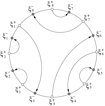
Figure 4: A planar set of arcs on the disk with $2j$ points along the boundary, labeled by $\xi^{{}_{+}}_{1},\xi^{{}_{-}}_{1},\dots,\xi^{{}_{+}}_{j},\xi^{{}_{-}}_{j}$, and its dual tree graph. On the figure $j=8$. The arcs split the disk into $j+1$ windows. The non-trivial weights of the windows in the figure are $C_{2}(\xi^{{}_{+}}_{7},\xi^{{}_{-}}_{8},\xi^{{}_{+}}_{8},\xi^{{}_{-}}_{7})$, $C_{3}(\xi^{{}_{+}}_{1},\xi^{{}_{-}}_{3},\xi^{{}_{+}}_{4},\xi^{{}_{-}}_{6},\xi^{{}_{+}}_{7},\xi^{{}_{-}}_{8})$, $C_{3}(\xi^{{}_{+}}_{1},\xi^{{}_{-}}_{3},\xi^{{}_{+}}_{3},\xi^{{}_{-}}_{2},\xi^{{}_{+}}_{2},\xi^{{}_{-}}_{1}),$ $C_{2}(\xi^{{}_{+}}_{4},\xi^{{}_{-}}_{6},\xi^{{}_{+}}_{6},\xi^{{}_{-}}_{4})$, $C_{2}(\xi^{{}_{+}}_{6},\xi^{{}_{-}}_{4},\xi^{{}_{+}}_{5},\xi^{{}_{-}}_{5}).$

In order to evaluate the amplitude in the $E$ space, we have to perform the integral transformation (3.19) of the r.h.s. of (3.55). We believe, although we are not able to supply the proof now, that the relations (3.37) and (3.51) hold in fact for any $n$. If we introduce the winding parameters $y_{1},\dots,y_{2n-1},y_{2n}\equiv y_{0}$, determined up to a common translation $y_{2i}\to y_{2i}+a,\ y_{2i-1}\to y_{2i-1}-a$, and express the energies as

$$E^{+}_{i}=y_{2i-2}+y_{2i-1}\,,\qquad E^{-}_{i}=y_{2i-1}+y_{2i}\,,$$ (3.57)

we conjecture that for any $n$

$${\cal R}_{n}(E^{+}_{1},E^{-}_{1},\dots,E^{+}_{n},E^{-}_{n})={\tilde{\Lambda}}^{n-i(E^{+}_{1}+\dots E^{+}_{n})}\ \overline{G_{n}(\xi^{{}_{+}}_{1},\xi^{{}_{-}}_{1},\dots,\xi^{{}_{+}}_{n},\xi^{{}_{-}}_{n})\,,}$$ (3.58)

where

$$\xi^{{}_{+}}_{i}={\tilde{\Lambda}}^{1/2}\,e^{-{1\over 2}{\pi}y_{2i-2}},\qquad\xi^{{}_{-}}_{i}={\tilde{\Lambda}}^{1/2}\,e^{-{1\over 2}{\pi}y_{2i-1}}\qquad(i=1,\dots,n)\,.$$ (3.59)

The energies $E_{i}$ and the winding parameters $y_{i}$ are logarithmically divergent with the cutoff ${\tilde{\Lambda}}$. In terms of the finite shifted energies $\hat{\epsilon}^{\pm}_{i}$ the above relations reads

$$\hat{\epsilon}^{+}_{i}=\hat{y}_{2i-2}+\hat{y}_{2i-1}\,,\qquad\hat{\epsilon}^{-}_{i}=\hat{y}_{2i-1}+\hat{y}_{2i}\,,$$ (3.60)

$$\xi^{{}_{+}}_{i}=\mu^{1/2}\,e^{-{1\over 2}{\pi}\hat{y}_{2i-2}},\qquad\xi^{{}_{-}}_{i}=\mu^{1/2}\,e^{-{1\over 2}{\pi}\hat{y}_{2i-1}}\qquad(i=1,\dots,n)\,.$$ (3.61)

From the perspective of the worldsheet theory, each term in the solution (3.55) is the contribution of a particular scattering process involving $n$ long strings sharing a common worldsheet. The arcs in the rainbow diagram on Figure 4 correspond to the tips of the $n$ long strings. The factorization of the amplitude means that the interaction occurs only in the far past ( $t\sim-\log\mu_{{}_{B}}$) or in the future ( $t\sim\log\mu_{{}_{B}}$). For $-\log\mu_{{}_{B}}\ll t\ll\log\mu_{{}_{B}}$ the $n$ long strings evolve independently, contributing a product of reflection factors ${\cal R}_{1}$. Furthermore, the recurrence relation (2) for the coefficients $C_{j}$ means that each such coefficient can be written as a sum of prodicts of $C_{2}$. Therefore the interaction of the long strings can be decomposed into exchanges of short strings as those illustrated in Figure 2.

4 Discussion

In this paper we studied the simplest scattering processes of long folded strings in the two-dimensional string theory. We used the description of the long strings in terms of a FZZT brane with $\mu_{{}_{B}}\gg\sqrt{\mu}$, as suggested in [1]. We evaluated the four-point disk amplitude in Maldacena’s limit of large momenta and large boundary parameters. We observed that the amplitude depends only on the chiral combinations $\hat{y}_{i}=y_{i}-s_{i}$, where $s_{a}$ are the Liouville boundary parameters and $y_{a}$ the “winding parameters” , associated with the four segments of the boundary ($a=1,2,3,4$). Furthermore we observed a symmetry with respect to the Fourier transformation in the time direction. Our result suggests that, to the leading order, the long strings interact via exchange of short open strings that happens in the asymptotically free region $\phi\ll-\log\mu$.

On the side of MQM the scattering amplitudes are expressed in terms of the mixed trace correlators in an effective non-compact two-matrix model with interaction $i{\rm tr\,}\mathbf{X}_{{}_{+}}\mathbf{X}_{{}_{-}}$. However the worldsheet interpretation of the correlation functions is not the same as in the matrix model description of rational $c<1$ string theories. In our case the spectral parameter $\xi^{{}_{\pm}}$ is related by Fourier transformation to the energy of the boundary tachyon, while the boundary condition for the Liouville field is determined by a regularization parameter ${\tilde{\Lambda}}$, the depth of the fermi sea. This is because the boundary is associated to the gauge field ${\bf A}$, while the fields $\mathbf{X}_{{}_{\pm}}$ create the asymptotic open string states. Since we are modelling a Lorentzian theory, the worldsheet description does not have a statistical interpretation as a sum over surfaces with positive weights.

We evaluated the subleading amplitude for any number $n$ of long strings using the results for the single-trace mixed correlator in the two-matrix model [20]. We obtained the result in the coordinate space, while the worldsheet calculation gives it in the space of energies. We performed explicitly the Fourier transformation for the cases $n=1$ and $n=2$ where we reproduced the result of the worldsheet theory up to factors that can be absorbed into the normalization of the boundary tachyons and the integration measure.

We found that the Fourier transformed amplitude takes essentially the same form as that in the coordinate space, after being expressed in terms of the $2n$ dual coordinates $y_{i}$ associated with the boundaries of the disk. We were able to establish this symmetry only for the cases $n=1$ and $n=2$, but we believe that it is a general property of the disk $n$-point amplitude in Maldacena’s limit.

Eventually we are interested taking the limit with a large number of FZZT branes, which would help us, as suggested in [1], to find a matrix model description of the Lorentzian black hole. The results reported in this paper suggest that the effective two-matrix model that stems from the chiral quantization of MQM is the right tool to achieve this limit. In this paper we studied the interactions of long folded strings due to exchange of short open strings, which are described by the single-trace mixed correlators in the effective two-matrix model. We did not consider the interactions due to the exchange of closed strings. Such interactions are described by multi-trace mixed correlators in the effective two-matrix model.

Acknowledgments

We thank S. Alexandrov and N. Orantin for valuable discussions. This work has been partially supported by the European Union through ENRAGE network (contract MRTN-CT-2004-005616), ANR programs GIMP (contract ANR-05-BLAN-0029-01). Part of this work was done during the “Integrability, Gauge Fields and Strings” focused research group at the Banff International Research Station.

Appendix A Properties of the functions ${\bf S}(z)$ and $f(x)$

We give here a short summary of the properties of the double sine function ${\bf S}(z)$ used in [16] and the function $f(x)$ introduced (for $b=1$) in [1]. The double sine is related to the double gamma function introduced by Barnes [39]. The function $e_{b}(x)=e^{if(\pi x)}$ is also known as non-compact quantum dilogarithm [40].

A.1 The double sine function ${\bf S}(z)$

• Integral representation: [16]

  $$\log{{\bf S}}(Q/2-ix)\,=\,{i\over 2}\int\limits_{0}^{\infty}\left(\frac{\sin 2tx}{\sinh bt\,\sinh{b^{-1}t}}-{2x\over t}\right)\,\frac{dt}{t}\,,\qquad Q=b+1/b\,.$$ (A.1)

• Functional relations:

  $$\frac{{\bf S}(z+b)}{{\bf S}(z)}={2\sin{\textstyle\pi bz}}\,,\quad\frac{{\bf S}(z+1/b)}{{\bf S}(z)}={2\sin\frac{\textstyle\pi z}{b}}\,.$$ (A.2)

• Poles and zeroes:

  $$\mbox{poles at}\ \ z=n_{1}b+n_{2}/b,\;\;n_{1},n_{2}\leq 0,\quad\mbox{zeroes at}\ \ z=n_{1}b+n_{2}/b,\;\;n_{1},\ n_{2}\geq 1\,.$$

• Asymptotics at infinity (for ${\rm Re}b>0$):

  $${\bf S}(x)~{}\sim~{}\exp\left({\mp i\pi}/{2}\left\{\left(x-{\textstyle{\frac{1}{2}}}Q\right)^{2}-{\textstyle\frac{1}{12}(b^{2}+b^{-2})}\right\}\right)~{}~{}~{}~{}~{}~{}~{}~{}({\rm Im}x\to\pm\infty)\,.$$ (A.3)

A.2 The function $f(x)$

• Definition:

  $$e^{if(x)}={e^{i{x^{2}/2\pi}+i\pi(b^{2}+b^{-2})/24}\over{\bf S}(Q/2-ix/\pi)}\,.$$ (A.4)

• Integral representation:

  $$f(x)=-{i\over 4}\int_{{\mathbb{R}}+i0}{dt\over t}\,{e^{-2itx/\pi}\over\sinh tb\,\sinh t/b}\,.$$ (A.5)

• Functional equations:

  $$f(x)+f(-x) = {x^{2}\over\pi}+{\pi(b^{2}+b^{-2})\over 12}\,,$$ (A.6)

  $$e^{if(x+i\pi b)} = {e^{if(x)}\over 1+e^{i\pi b^{2}}e^{2bx}}\,,$$ (A.8)

  $$e^{if(x+i\pi/b)} = {e^{if(x)}\over 1+e^{i\pi/b^{2}}e^{2x/b}}\,.$$ (A.10)

• Asymptotics at infinity (for $b>0$):

  $$f(x)\;\to\;\left\{\begin{array}[]{ll}0,&\Re x\to-\infty\\ x^{2}/\pi+\pi(b^{2}+b^{-2})/12\ ,&\Re x\to+\infty\,.\end{array}\right.$$ (A.13)

• Fourier transform [41, 42]

  $$\int_{{\mathbb{R}}}{dt\over\pi}\,e^{-Qt}\ e^{if(-t)}\,e^{2itx/\pi} = e^{-i\alpha}\;e^{Qx}\ e^{-if(x)}\;$$ (A.14)

  $$\int_{{\mathbb{R}}}{dt\over\pi}\,e^{-Qt}\ e^{-if(-t)}\,e^{2itx/\pi} = e^{i\alpha}\;e^{-Qx}\ e^{if(-x)}\;$$ (A.16)

  $$\int_{{\mathbb{R}}}{dt\over\pi}\,e^{Qt}\ e^{if(t)}\,e^{2itx/\pi} = e^{-i\alpha}\;e^{-Qx}\ e^{-if(-x)}\;$$ (A.18)

  $$\int_{{\mathbb{R}}}{dt\over\pi}\,e^{Qt}\ e^{-if(t)}\,e^{2izt/\pi} = e^{i\alpha}\;e^{Qx}\ e^{if(x)}\;$$ (A.20)

  where $\alpha=\pi{1+Q^{2}\over 12}-\pi{Q^{2}\over 4}$.

A.3 The limit $b\to 1$

• Integral representation:

  Evaluating the derivative

  $$\frac{d}{dx}\log{\bf S}(1-ix)|_{b=1}~{}=~{}i\int_{0}^{\infty}dt\left[\frac{\cos 2tx}{\sinh^{2}t}-\frac{1}{t^{2}}\right]~{}=~{}\frac{-i\pi x}{\tanh\pi x}.$$ (A.21)

  we find another integral representation of the dounle sine for $b=1$:

  $$i\pi\log{\bf S}(1-ix)|_{b=1}~{}=~{}\pi\int_{0}^{x}dx^{\prime}\frac{\pi x^{\prime}}{\tanh\pi x^{\prime}}~{}=~{}\int_{0}^{\pi x}d\zeta\frac{\zeta}{\tanh\zeta}.$$ (A.22)

  Then (A.4) reproduces the function $f(x)$ as defined in [18]:

  $$f(x)~{}=~{}\frac{1}{\pi}\int_{-\infty}^{x}d\zeta\left(\frac{\zeta}{\tanh\zeta}+\zeta\right).$$ (A.23)

• Functional equations:

  $$f(x)+f(-x) = {x^{2}\over\pi}+{\pi\over 6}\,,$$ (A.24)

  $$\qquad e^{if(x-i\pi)}=(1-e^{2x})\,e^{if(x)}\,,$$ (A.25)

  
  

• Boundary reflection coefficient $d(k,s,s^{\prime})|_{b=1}$:

  $$d(k,s,s^{\prime}) \stackrel{{\scriptstyle b=1}}{{=}} {\bf S}(1+2ik){\bf S}(1-i(k+s+s^{\prime})){\bf S}(1-i(k+s-s^{\prime}))$$ (A.26)

  $$\hskip 39.83385pt\times\,{\bf S}(1-i(k-s+s^{\prime})){\bf S}(1-i(k-s-s^{\prime})).$$

  $$\left.d(k,s,s^{\prime})^{\pm 1}\right|_{(k,s,s^{\prime})\sim(\pm 2M,M,M)} = e^{-2\pi i(s^{2}+s^{\prime 2})-\frac{i\pi}{4}+if(\pi s+\pi s^{\prime}\mp\pi k)}.$$ (A.27)

Appendix B Equation for the boundary Liouville three point function

Here we derive a shift equation for the three-point function of boundary operators $B_{\beta}\equiv e^{\beta\phi}$ in Liouville theory on a disk. We denote the relevant structure constant by $C^{\beta_{1},\beta_{2},\beta_{3}}_{~{}s_{1},s_{2},s_{3}}$:

$$\left\langle{B_{\beta_{1}}(x_{1})B_{\beta_{2}}(x_{2})B_{\beta_{3}}(x_{3})}\right\rangle_{s_{1},s_{2},s_{3}} = C^{\beta_{1},\beta_{2},\beta_{3}}_{~{}s_{1},s_{2},s_{3}}\prod_{\{ijk\}}|x_{i}-x_{j}|^{h_{k}-h_{i}-h_{j}}.$$

Our notation is such that $B_{\beta_{1}}$ joins the branes $s_{3}$ and $s_{1}$, $B_{\beta_{2}}$ joins $s_{1}$ and $s_{2}$ and so on. The shift equation follows from the bootstrap constraints of four-point functions containing one boundary degenerate operator $B_{-b/2}$ or $B_{-1/2b}$. Note that the two branes joined by $B_{-b/2}$ have to satisfy [16]

$$s-s^{\prime}=\pm ib/2~{}~{}~{}~{}{\rm or}~{}~{}~{}~{}s+s^{\prime}=\pm ib/2,$$

and similarly for those joined by $B_{-1/2b}$.

To recall where the constraints arise from, let us consider a four-point function,

$$\left\langle{B_{\beta_{1}}(x_{1})B_{-b/2}(x)B_{\beta_{2}}(x_{2})B_{\beta_{3}}(x_{3})}\right\rangle_{s^{\prime}_{1},s_{1},s_{2},s_{3}}.$$

Using the analytic solutions of Virasoro Ward identity with the knowledge of the operator product expansions involving $B_{-b/2}$, one can derive linear relations among $C^{\beta_{1}\mp b/2,\beta_{2},\beta_{3}}_{s_{1},s_{2},s_{3}}$ and $C^{\beta_{1},\beta_{2}\mp b/2,\beta_{3}}_{s^{\prime}_{1},s_{2},s_{3}}$. One of them reads, after replacing $\beta_{i}$ by $\frac{Q}{2}-ik_{i}$,

$$-\frac{\Gamma(1-2ibk_{1})}{\Gamma(\alpha-2ibk_{1})}\,C^{\frac{Q}{2}-ik_{1}-\frac{b}{2},\frac{Q}{2}-ik_{2},\frac{Q}{2}-ik_{3}}_{s_{1},s_{2},s_{3}}+\frac{\Gamma(1+2ibk_{2}-\alpha)}{\Gamma(2ibk_{2})}\,C^{\frac{Q}{2}-ik_{1},\frac{Q}{2}-ik_{2}-\frac{b}{2},\frac{Q}{2}-ik_{3}}_{s^{\prime}_{1},s_{2},s_{3}}$$

$$~{}=~{}\frac{\Gamma(1+2ibk_{1})\Gamma(1+2ibk_{2}-\alpha)}{\Gamma(1+2ibk_{1}+2ibk_{2}-\alpha)\Gamma(\alpha)}\,\frac{d_{L}(\frac{Q}{2}-ik_{1},s_{3},s_{1}^{\prime})}{d_{L}(\frac{Q}{2}-ik_{1}+\frac{b}{2},s_{3},s_{1})}\,C^{\frac{Q}{2}-ik_{1}+\frac{b}{2},\frac{Q}{2}-ik_{2},\frac{Q}{2}-ik_{3}}_{s_{1},s_{2},s_{3}}.$$

Here $\alpha\equiv\frac{1}{2}+ib(k_{1}+k_{2}+k_{3})$, and $d_{L}$ is defined in (2.8). See [24] and [43] for more detail. A similar relation is obtained from the four-point function containing $B_{-1/2b}$. This kind of shift relations among correlators is often powerful enough to determine the structure constants in Liouville theory.

We translate the above relations on Liouville correlators into a shift relation among the disk amplitudes of three $U^{-}_{k}$ or three $U^{-}_{k}$ in two-dimensional string theory. The conservation of energy requires $k_{1}+k_{2}+k_{3}=-\tilde{Q}/2$ or $\alpha=0$ in the above. We will suppress the corresponding delta function when writing down the formulae for amplitudes. The divergence of $\Gamma(\alpha)$ in the right hand side is canceled by the bulk divergence [24] of $C^{\beta_{1},\beta_{2},\beta_{3}}_{s_{1},s_{2},s_{3}}$ at $\beta_{1}+\beta_{2}+\beta_{3}=2Q$:

$$C^{\beta_{1},\beta_{2},\beta_{3}}_{s_{1},s_{2},s_{3}} \sim \frac{d_{L}(\beta_{1},s_{3},s_{1})d_{L}(\beta_{2},s_{1},s_{2})d_{L}(\beta_{3},s_{2},s_{3})}{2Q-\beta_{1}-\beta_{2}-\beta_{3}}.$$

So we obtain (2.12) and (2.13).

Appendix C Derivation of the correlator $G_{2}$ (3.41).

To evaluate the correlator $G_{2}$ we use the identity, following from the translation invariance of the matrix measure,

$$\int d\mathbf{X}_{{}_{+}}d\mathbf{X}_{{}_{-}}{\rm tr\,}(\nabla_{\!{}_{+}}W\!_{\!{}_{+}}^{\ 2}W\!_{\!{}_{-}}^{\ 2}W\!_{\!{}_{+}}^{\ 1}W\!_{\!{}_{-}}^{\ 1})\,\Phi_{0}^{+}\Phi_{0}^{-}\,\ e^{i{\rm tr\,}{X_{+}X_{-}}}=0.$$ (C.1)

Here $\nabla_{\!{}_{\pm}}=\partial_{\mathbf{X}_{{}_{\pm}}}$ is the operator of matrix derivative, $\Phi_{0}^{+}(\mathbf{X}_{{}_{+}})$ and $\Phi_{0}^{-}(\mathbf{X}_{{}_{-}})$ are the wave functions of the left and right ground states in the singlet sector and $W\!_{\!{}_{\pm}}^{\ a}\,(a=1,2)$ denote resolvents (3.18) with spectral parameters $\xi^{{}_{\pm}}_{a}$:

$$W\!_{\!{}_{\pm}}^{\ a}\equiv W\!_{\!{}_{\pm}}(\xi^{{}_{\pm}}_{a})={1\over\xi^{{}_{\pm}}_{a}+\mathbf{X}_{{}_{\pm}}}\,.$$

We commute the operator of derivative to the right using that it acts on the resolvents as $[\nabla_{\!{}_{\pm}}]_{j}^{k}\cdot[W\!_{\!{}_{\pm}}^{\ a}]_{j^{\prime}}^{k^{\prime}}=-[W\!_{\!{}_{\pm}}^{\ a}]_{j^{\prime}}^{k}\,[W\!_{\!{}_{\pm}}^{\ a}]_{j}^{k^{\prime}}$. As a result we obtain the identity

$$\left\langle\,\!\mu\left|\,-{\rm tr\,}W\!_{\!{}_{+}}^{\ 2}\,{\rm tr\,}(W\!_{\!{}_{+}}^{\ 2}W\!_{\!{}_{-}}^{\ 2}W\!_{\!{}_{+}}^{\ 1}W\!_{\!{}_{-}}^{\ 1})-{\rm tr\,}(W\!_{\!{}_{+}}^{\ 2}W\!_{\!{}_{-}}^{\ 2}W\!_{\!{}_{+}}^{\ 1})\,{\rm tr\,}(W\!_{\!{}_{+}}^{\ 1}W\!_{\!{}_{-}}^{\ 1})\,\right|\mu\!\,\right\rangle$$ (C.2)

$$+\left\langle\,\!\mu\left|\,{\rm tr\,}(W\!_{\!{}_{+}}^{\ 2}W\!_{\!{}_{-}}^{\ 2}W\!_{\!{}_{+}}^{\ 1}W\!_{\!{}_{-}}^{\ 1}(i\mathbf{X}_{{}_{-}}+\nabla_{\!{}_{+}}\ln\Phi_{0}^{+}\,\right|\mu\!\,\right\rangle=0.$$ (C.3)

In a similar way, replacing the trace in (C.1) with ${\rm tr\,}(\nabla_{\!{}_{+}}W\!_{\!{}_{-}}^{\ 2}W\!_{\!{}_{+}}^{\ 1}W\!_{\!{}_{-}}^{\ 1}W\!_{\!{}_{+}}^{\ 2})$, we obtain another identity,

$$\left\langle\,\!\mu\left|\,-{\rm tr\,}(W\!_{\!{}_{-}}^{\ 2}W\!_{\!{}_{+}}^{\ 1})\,{\rm tr\,}(W\!_{\!{}_{+}}^{\ 1}W\!_{\!{}_{-}}^{\ 1}W\!_{\!{}_{+}}^{\ 2})-{\rm tr\,}(W\!_{\!{}_{-}}^{\ 2}W\!_{\!{}_{+}}^{\ 1}W\!_{\!{}_{-}}^{\ 1}W\!_{\!{}_{+}}^{\ 2})\,{\rm tr\,}W\!_{\!{}_{+}}^{\ 2})\,\right|\mu\!\,\right\rangle$$ (C.4)

$$+\left\langle\,\!\mu\left|\,{\rm tr\,}(W\!_{\!{}_{-}}^{\ 2}W\!_{\!{}_{+}}^{\ 1}W\!_{\!{}_{-}}^{\ 1}W\!_{\!{}_{+}}^{\ 2}(i\mathbf{X}_{{}_{-}}+\nabla_{\!{}_{+}}\ln\Phi_{0}^{+}\,\right|\mu\!\,\right\rangle=0.$$ (C.5)

Now we subtract (C.5) from (C.3) and use that $[W\!_{\!{}_{+}}^{\ 2},\nabla_{\!{}_{+}}\ln\Phi_{0}^{+}]=0$. As a result we have an identity that does not involve the ground state wave function:

$$\left\langle\,\!\mu\left|\,{\rm tr\,}(W\!_{\!{}_{+}}^{\ 1}W\!_{\!{}_{-}}^{\ 2})\,{\rm tr\,}(W\!_{\!{}_{+}}^{\ 2}W\!_{\!{}_{+}}^{\ 1}W\!_{\!{}_{-}}^{\ 1})-{\rm tr\,}(W\!_{\!{}_{+}}^{\ 1}W\!_{\!{}_{+}}^{\ 2}W\!_{\!{}_{-}}^{\ 2})\,{\rm tr\,}(W\!_{\!{}_{+}}^{\ 1}W\!_{\!{}_{-}}^{\ 1})\,\right|\mu\!\,\right\rangle$$ (C.6)

$$+i\left\langle\,\!\mu\left|\,{\rm tr\,}(W\!_{\!{}_{+}}^{\ 2}W\!_{\!{}_{-}}^{\ 2}W\!_{\!{}_{+}}^{\ 1}W\!_{\!{}_{-}}^{\ 1}\mathbf{X}_{{}_{-}})-{\rm tr\,}(\mathbf{X}_{{}_{-}}W\!_{\!{}_{-}}^{\ 2}W\!_{\!{}_{+}}^{\ 1}W\!_{\!{}_{-}}^{\ 1}W\!_{\!{}_{+}}^{\ 2})\,\right|\mu\!\,\right\rangle=0.$$ (C.7)

Applying the identities

$$W\!_{\!{}_{\pm}}^{\ 1}W\!_{\!{}_{\pm}}^{\ 2}=-\,\frac{W\!_{\!{}_{\pm}}^{\ 1}-W\!_{\!{}_{\pm}}^{\ 2}}{\xi^{{}_{\pm}}_{1}-\xi^{{}_{\pm}}_{2}},\qquad\mathbf{X}_{{}_{\pm}}W\!_{\!{}_{\pm}}^{\ a}=1-\xi^{{}_{\pm}}W\!_{\!{}_{\pm}}^{\ a}\,$$

we write (C.7) as

$$\langle\mu|\frac{{\rm tr\,}(W\!_{\!{}_{+}}^{\ 1}W\!_{\!{}_{-}}^{\ 2})\,{\rm tr\,}(W\!_{\!{}_{+}}^{\ 2}W\!_{\!{}_{-}}^{\ 1})-{\rm tr\,}(W\!_{\!{}_{+}}^{\ 1}W\!_{\!{}_{-}}^{\ 1}){\rm tr\,}(W\!_{\!{}_{+}}^{\ 2}W\!_{\!{}_{-}}^{\ 2})}{\xi^{{}_{+}}_{1}-\xi^{{}_{+}}_{2}}|\mu\rangle$$ (C.8)

(C.9)

$$-i\langle\mu|\frac{{\rm tr\,}(W\!_{\!{}_{+}}^{\ 1}W\!_{\!{}_{-}}^{\ 2}-W\!_{\!{}_{+}}^{\ 2}W\!_{\!{}_{-}}^{\ 2}-W\!_{\!{}_{+}}^{\ 1}W\!_{\!{}_{-}}^{\ 1}+W\!_{\!{}_{+}}^{\ 2}W\!_{\!{}_{-}}^{\ 1})}{\xi^{{}_{+}}_{1}-\xi^{{}_{+}}_{2}}|\mu\rangle$$ (C.10)

(C.11)

$$-i\left\langle\,\!\mu\left|\,{\rm tr\,}(W\!_{\!{}_{+}}^{\ 1}W\!_{\!{}_{-}}^{\ 1}W\!_{\!{}_{+}}^{\ 2}W\!_{\!{}_{-}}^{\ 2})(\xi^{{}_{+}}_{1}-\xi^{{}_{+}}_{2})\,\right|\mu\!\,\right\rangle\,=0\,.$$ (C.12)

In the leading order in the $1/\mu$ expansion we can use the factorization of the normalized expectation values, $\left\langle\,\!\mu\left|\,{\rm tr\,}A\,{\rm tr\,}B\,\right|\mu\!\,\right\rangle=\left\langle\,\!\mu\left|\,{\rm tr\,}A\,\right|\mu\!\,\right\rangle\left\langle\,\!\mu\left|\,{\rm tr\,}B\,\right|\mu\!\,\right\rangle$. Setting

$$G_{2}(\xi_{1}^{+},\xi_{1}^{-},\xi_{2}^{+},\xi_{2}^{-})=\left\langle\,\!\mu\left|\,{\rm tr\,}{W\!_{\!{}_{+}}^{\ 1}W\!_{\!{}_{-}}^{\ 1}W\!_{\!{}_{+}}^{\ 2}W\!_{\!{}_{-}}^{\ 2}}\,\right|\mu\!\,\right\rangle,$$

$$G_{1}(\xi^{+},\xi^{-})=\left\langle\,\!\mu\left|\,{\rm tr\,}(W\!_{\!{}_{+}}W\!_{\!{}_{-}})\,\right|\mu\!\,\right\rangle-i,$$

we retrieve (3.41):

$$G_{2}(\xi_{1}^{+},\xi_{1}^{-},\xi_{2}^{+},\xi_{2}^{-})=i\,\frac{G_{1}(\xi_{1}^{+},\xi_{1}^{-})G_{1}(\xi_{2}^{+},\xi_{2}^{-})-G_{1}(\xi_{1}^{+},\xi_{2}^{-})G_{1}(\xi_{2}^{+},\xi_{1}^{-})}{(\xi_{2}^{+}-\xi_{1}^{+})(\xi_{2}^{-}-\xi_{1}^{-})}\,.$$

Proceeding in the same way one obtains a recursive formula for the one-trace correlator $G_{n}$ [20]

$${G}_{n}(\xi^{{}_{+}}_{1},\xi^{{}_{-}}_{1},\dots,\xi^{{}_{+}}_{n},\xi^{{}_{-}}_{n}) =i\sum_{j=1}^{k-1}\frac{{G}_{j}(\xi^{{}_{+}}_{1},\xi^{{}_{-}}_{1},\dots,\xi^{{}_{+}}_{j},\xi^{{}_{-}}_{j}){G}_{k-j}(\xi^{{}_{+}}_{j+1},\xi^{{}_{-}}_{j+1},\dots,\xi^{{}_{+}}_{k},\xi^{{}_{-}}_{n})}{(\xi^{{}_{-}}_{n}-\xi^{{}_{-}}_{j})(\xi^{{}_{+}}_{k}-\xi^{{}_{+}}_{1})}$$

$$\ -i\sum_{j=1}^{n-1}{{G}_{j}(\xi^{{}_{+}}_{1},\xi^{{}_{-}}_{1},\dots,\xi^{{}_{+}}_{j},\xi^{{}_{-}}_{k}){G}_{n-j}(\xi^{{}_{+}}_{j+1},\xi^{{}_{-}}_{j+1},\dots,\xi^{{}_{+}}_{k},\xi^{{}_{-}}_{j})\over(\xi^{{}_{-}}_{k}-\xi^{{}_{-}}_{j})(\xi^{{}_{+}}_{n}-\xi^{{}_{+}}_{1})}\,.$$

Appendix D Evaluation of the integral for $R_{2}(E_{1}^{+},E_{2}^{+},E_{1}^{-},E_{2}^{-})$

In order to evaluate the disk scattering amplitude in the space of energies, we need to perform the integral transformation (3.19) with respect to all four variables of the amplitude (3.41):

$$R_{2}(E^{+}_{1},E^{+}_{2},E^{-}_{1},E^{-}_{2})=\frac{1}{\pi^{4}}\sinh\pi E^{+}_{1}\ \sinh\pi E^{+}_{2}\ \sinh\pi E^{-}_{1}\ \sinh\pi E^{-}_{2}$$ (D.1)

$$\times\int_{0}^{\infty}d\xi^{{}_{+}}_{1}d\xi^{{}_{+}}_{2}d\xi^{{}_{-}}_{1}d\xi^{{}_{-}}_{2}\ \,(\xi^{{}_{+}}_{1})^{-iE_{1}^{+}}(\xi^{{}_{+}}_{2})^{-iE_{2}^{+}}(\xi^{{}_{-}}_{1})^{-iE_{1}^{-}}(\xi^{{}_{-}}_{2})^{-iE_{2}^{-}}\ G_{2}(\xi_{1}^{+},\xi_{2}^{+},\xi_{1}^{-},\xi_{2}^{-})\,.$$ (D.2)

We will use the fact that the integral transform of the two factors $G_{1}$ in the expression (3.41) for $R_{2}$ is already known. We express the r.h.s. of (D.2) in terms of

$$R_{1}(E^{+},E^{-})=\delta(E^{+}-E^{-})\,{\cal R}_{1}(E^{+})$$ (D.3)

by applying the inverse transformation (3.20):

$$G_{1}(\xi^{+},\xi^{-}) = -{1\over 4\xi^{+}\xi^{-}}\int\limits_{{\mathbb{R}}+i/2}{dE^{+}\over\sinh\pi E^{+}}\ \xi_{+}^{iE^{+}}{dE^{-}\over\sinh\pi E^{-}}\ \xi_{-}^{iE^{-}}{\cal R}_{1}(E^{+},E^{-}).$$ (D.4)

As a result, the original integral takes the form

$$R_{2} = \int_{{\mathbb{R}}+i/2}\prod_{\pm}[dp^{\pm}_{1}dp^{\pm}_{2}\ \ K(E^{\pm}_{1},E^{\pm}_{2};p^{\pm}_{1},p^{\pm}_{2})]\ {\cal R}_{1}(p_{1}^{+},p_{1}^{-})\,{\cal R}_{1}(p_{2}^{+},p_{2}^{-})\,\,,$$

where the kernel $K(E_{1},E_{2};y_{1},y_{2})$ is given by the integral

$$K(E_{1},E_{2};p_{1},p_{2}) = \frac{A}{2\pi^{2}}\int_{0}^{\infty}{d\xi_{1}d\xi_{2}\over\xi_{1}\,\xi_{2}}\ \ {\det\limits_{jk}\xi_{j}^{i(p_{k}-E_{j})}\over\xi_{1}-\xi_{2}}\ \,.$$ (D.6)

The factor

$$A=\prod_{j=1,2}{\sinh\pi E_{j}\over\sinh\pi p_{j}}$$ (D.7)

can be put equal to 1, as we will see later. To evaluate the kernel, change the variables as $\xi_{1}=e^{\tau+t},\ \ \xi_{2}=e^{\tau-t}$,

$$\hskip-14.22636ptA^{-1}\,K(E_{1},E_{2};p_{1},p_{2}) = {i\over\pi^{2}}\,\int_{-\infty}^{\infty}d\tau dt\,e^{i\tau(p_{1}+p_{2}-E_{1}-E_{2})}e^{it(E_{2}-E_{1})}\ {\sin(p_{2}-p_{1})t\over e^{\tau}\sinh t}$$ (D.8)

$$= {2\over\pi}i\,\delta(E_{1}+E_{2}-p_{1}-p_{2}+i)\ \int_{-\infty}^{\infty}dt\ {\cos(E_{1}-E_{2})t\ \sin(p_{1}-p_{2})t\over\sinh t}$$

$$= 2\,i\,\delta(E_{1}+E_{2}-p_{1}-p_{2}+i)\ {\sinh\pi(p_{1}-p_{2})\over\cosh\pi(E_{1}-E_{2})+\cosh\pi(p_{1}-p_{2})}\,.$$

After substituting (LABEL:Kpm) and (D.3) in the integral (D), three of the integrations are compensated by $\delta$-functions, the remaining $\delta$-function imposes the conservation of the total energy:

$$R_{2}(E^{+}_{1},E^{+}_{2},E^{-}_{1},E^{-}_{2})=\delta(E^{+}_{1}+E^{+}_{2}-E^{-}_{1}-E^{-}_{2})\,{\cal R}_{2}.$$ (D.11)

It is convenient to introduce the independent variables $E,\Delta_{\pm}$ and $\epsilon^{\prime}$ by

$$E^{\pm}_{1}=E+{\Delta_{\pm}},\ \ \ E^{\pm}_{2}=E-{\Delta_{\pm}},\ \ \ \ p_{1}=E+\epsilon^{\prime}+{\textstyle{\frac{1}{2}}}i,\ \ p_{2}=E-\epsilon^{\prime}+{\textstyle{\frac{1}{2}}}i\,,$$ (D.12)

$\epsilon^{\prime}$ being the integration variable. It is clear that in the Maldacena limit

$$E={1\over 2\pi}\ln\Lambda+\epsilon$$ (D.13)

with $\epsilon,\Delta_{\pm}$ finite, the factor (D.7) can be replaced by 1. Then we can write the remaining integral as

$${\cal R}_{2}=4i\,\int_{-\infty}^{\infty}d\epsilon^{\prime}\ {\frac{\sinh^{2}{2\pi\epsilon^{\prime}}\ \ {{\cal R}_{1}}(E+\epsilon^{\prime}+{\textstyle{\frac{1}{2}}}i){{\cal R}_{1}}(E-\epsilon^{\prime}+{\textstyle{\frac{1}{2}}}i)}{(\cosh{2\pi\Delta_{+}}+\cosh{2\pi\epsilon^{\prime}})(\cosh{2\pi{\Delta}_{-}}+\cosh{2\pi\epsilon^{\prime}})}}.$$ (D.14)

We are going to evaluate the integral (D.14) as a contour integral. According to (3.33) the integrand behaves at $\epsilon^{\prime}\to\pm\infty$ as $\exp(-i\pi\epsilon^{\prime 2})$. This leads to the choice of a 8-like contour shown in Fig. 3. We will show later that the integral integration along the imaginary axis is zero, so that the integral (D.14) is given by the sum of the residues trapped inside the 8-shaped contour. The integrand contains two kinds of poles. First, there are the (simple) poles of the kernel at

$$\epsilon^{\prime}=\pm{\Delta}_{-}+(n+{\textstyle{\frac{1}{2}}})i,\ \pm{\Delta}_{+}+(n+{\textstyle{\frac{1}{2}}})i,\qquad n\in{\mathbb{Z}}.$$

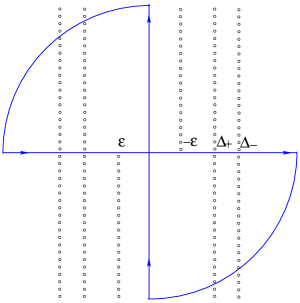
Figure 5: The 8-like contour in the $\epsilon^{\prime}$-plane and the pattern of the poles.

Second, there are the poles of the factors ${{\cal R}_{1}}(E\pm\epsilon^{\prime}+{\textstyle{\frac{1}{2}}}i)$ at

$$\epsilon^{\prime}=\mp\hat{\epsilon}\pm(n+{\textstyle{\frac{1}{2}}})i,\qquad n\in{\mathbb{Z}}_{+}\,,$$

where by $\hat{\epsilon}$ we denoted the shifted energy $\hat{\epsilon}=\epsilon+{1\over 2\pi}\ln\mu=E-{1\over 2\pi}\ln(\Lambda/\mu)$. The order of these poles grow linearly with $n$.

We will assume that $\hat{\epsilon}<0$. Then the second kind of poles remain outside the integration contour and the only contribution will come from the poles of the kernel. Let us sum up the contributions of the poles along the lines $\Re\epsilon=\pm\Delta_{-}$. Assume for definiteness that ${\Delta}_{-}>0$. Then we have to sum up the resudues at

$$\epsilon^{\prime}=\pm{\Delta}_{-}\mp(n+{\textstyle{\frac{1}{2}}})i,\quad n\in{\mathbb{Z}}_{+}.$$ (D.15)

The residues of the kernel are the same for all poles:

$${\rm Res}K=i\,\frac{\sinh{2\pi\Delta_{-}}}{2\pi(\cosh{2\pi\Delta_{+}}-\cosh{2\pi\Delta_{-}})}\,.$$ (D.16)

The factor ${{\cal R}_{1}}{{\cal R}_{1}}$ in the integrand is evaluated at the $n$-th pole using the shifting property

$${{\cal R}_{1}}(E+ni)=\mu^{-n}(1-e^{-2\pi\hat{\epsilon}})^{-n}\,{{\cal R}_{1}}(E)=(\mu-e^{-2\pi\epsilon})^{-n}\,{{\cal R}_{1}}(E)\,.$$ (D.17)

The sum over the poles yields a factor

$$\sum_{n\in\mathbb{Z}_{+}}{{\cal R}_{1}(E+\Delta_{-}-ni){\cal R}_{1}(E-\Delta_{-}+(n+1)i)}$$ (D.18)

$$=\frac{{\cal R}_{1}(E+\Delta_{-}){\cal R}_{1}(E-\Delta_{-})}{\mu(1-e^{-2\pi(\hat{\epsilon}-\Delta_{-})})}\sum_{n=0}^{\infty}{\left(\frac{1-e^{-2\pi(\hat{\epsilon}+\Delta_{-})}}{1-e^{-2\pi(\hat{\epsilon}-\Delta_{-})}}\right)^{n}}$$ (D.19)

$$=-e^{2\pi\epsilon}\ {{\cal R}_{1}(E+\Delta_{-}){\cal R}_{1}(E-\Delta_{-})\over 2\sinh 2\pi\Delta_{-}}\,.$$ (D.20)

Taking into account the contribution of both series of poles (D.15) we get

$${\cal R}_{2}|_{{\rm poles}\ {\Delta}_{-}}=-{2}\,e^{2\pi\epsilon}\ \frac{{\cal R}_{1}(E+{\Delta}_{-}){\cal R}_{1}(E-{\Delta}_{-})}{\cosh{2\pi{\Delta}_{+}}-\cosh{2\pi{\Delta}_{-}}}\,.$$ (D.21)

Similarly we evaluate the contribution of the poles with $\Re\epsilon=\pm\Delta_{+}$. Returning to the original variables $E^{\pm}_{j}$ we write the final result as

$${{\cal R}}_{2}=-\frac{2}{\Lambda}\ e^{\pi(E^{+}_{1}+E^{+}_{2})}\ \frac{{{\cal R}_{1}}(E^{+}_{1}){{\cal R}_{1}}(E^{+}_{2})-{{\cal R}_{1}}(E^{-}_{1}){{\cal R}_{1}}(E^{-}_{2})}{\sinh{\pi(E^{+}_{1}-E^{-}_{1})}\sinh{\pi(E^{+}_{1}-E^{-}_{2})}}\,.$$ (D.22)

In terms of the renormalized energies (3.30), $\hat{\epsilon}^{\pm}_{j}=E^{\pm}_{j}-{1\over 2\pi}\ln(\Lambda/\mu)$ the result reads

$${{\cal R}}_{2}=-\frac{2}{\mu}\ e^{\pi(\hat{\epsilon}^{+}_{1}+\hat{\epsilon}^{+}_{2})}\ \frac{{{\cal R}_{1}}(E^{+}_{1}){{\cal R}_{1}}(E^{+}_{2})-{{\cal R}_{1}}(E^{-}_{1}){{\cal R}_{1}}(E^{-}_{2})}{\sinh{\pi(\hat{\epsilon}_{1}^{+}-\hat{\epsilon}_{1}^{-})}\sinh{\pi(\hat{\epsilon}_{1}^{+}-\hat{\epsilon}_{2}^{-})}}\,.$$ (D.23)

This expression can be safely analytically continued for $\hat{\epsilon}>0$. Note that the scattering amplitude (D.23) is of order $1/\mu$ compared to the leading order, as it should.

We still need to show that the integral over the imaginary axis, $\epsilon^{\prime}=iq$, vanishes. The integral in question is

$$I=\int_{-\infty}^{\infty}dq\,F(q),\qquad F(q)=4i\,\frac{\sin^{2}{2\pi q}\ {\cal R}_{1}(E+iq+{\textstyle{\frac{1}{2}}}i)){\cal R}_{1}(E-iq+{\textstyle{\frac{1}{2}}}i)}{(\cosh{2\pi{\Delta}_{+}}+\cos{2\pi q})(\cosh{2\pi{\Delta}_{-}}+\cos{2\pi q})}.$$ (D.24)

We split the interval into segments of length 1 and use the quasi-periodicity of the integrand:

$$I=\sum_{n\in{\mathbb{Z}}}\int_{-1/2}^{1/2}dqF(q+n)=\int_{-1/2}^{1/2}dq\sum_{n\in{\mathbb{Z}}}e^{in\phi(q)}\,F(q)\,,\quad e^{i\phi(q)}=\frac{e^{2\pi\hat{\epsilon}}-e^{2\pi iq}}{e^{2\pi\hat{\epsilon}}-e^{-2\pi iq}}\,.$$ (D.25)

The sum of the unitary numbers gives $e^{2\pi\hat{\epsilon}}\,\delta(q)$, so that indeed $I\sim F(0)=0$.

Appendix E Calogero Hamiltonian for general representations

In this appendix, we derive the explicit form of the Calogero Hamiltonian for arbitrary representation. In particular, we focus on the second part of the Hamiltonian (E.1) which is important in the continuum limit,

$$H_{1}=\frac{1}{2}\sum_{j\neq k}^{N}\frac{{\cal D}(E_{j}^{k}){\cal D}(E_{k}^{j})}{(x_{j}-x_{k})^{2}}\,.$$ (E.1)

In general, the wave function associated with the Young diagram whose box (resp. anti-box) part is described by $Y_{1}$ (resp. $Y_{2}$) is obtained by applying the Young symmetrizer associated with $Y_{1}$ to the upper indices and the Young symmetrizer associated with $Y_{2}$ to the lower indices and satisfies the tracesss condition for any pair of the upper and lower indices. More explicitly, if we write

$$\pi_{Y}=\sum_{\sigma\in S_{n}}\pi(Y,\sigma)\sigma$$ (E.2)

as the Young symmetrizer for the Young diagram $Y$, the state associated with the representation $Y_{1},Y_{2}$ can be written in terms of the adjoint wave functions as,

$$\Psi^{j_{1}\cdots j_{n}}_{k_{1}\cdots k_{n}}(\mathbf{X})=\sum_{\sigma,\tau\in S_{n}}\pi(Y_{1},\sigma)\pi(Y_{2},\tau)f_{1}(\mathbf{X})^{j_{\sigma(1)}}_{k_{\tau(1)}}\cdots f_{n}(\mathbf{X})^{j_{\sigma(n)}}_{k_{\tau(n)}}-\cdots\,.$$ (E.3)

Here, again, $\cdots$ represents the terms which are needed to keep the traceless condition for $\Psi^{j_{1}\cdots j_{n}}_{k_{1}\cdots k_{n}}(\mathbf{X})$.

For a general representation (E.3) we need to identify the index sets $j_{1},\cdots,j_{n}$ with $k_{1},\cdots,k_{n}$. In order to keep track of the original index structure, it will be useful to represent the state vector in the form

$$\sum_{j_{n},k_{n}}^{N}\Psi^{j_{1}\cdots j_{n}}_{k_{1}\cdots k_{n}}(\mathbf{X})|j_{1}\cdots j_{n}\rangle\langle k_{1},\cdots,k_{n}|$$

$$\quad\rightarrow\sum_{j_{n}}^{N}w_{j_{1}\cdots j_{n}}(x)|j_{1}\cdots j_{n}\rangle\langle j_{1},\cdots,j_{n}|$$ (E.4)

$$w_{j_{1}\cdots j_{n}}(x)=\Psi^{j_{1}\cdots j_{n}}_{j_{1}\cdots j_{n}}(x)$$ (E.5)

The element of the permutation on the upper (resp. lower) indices can be applied to the ket (resp. bra) state as,

$$\overrightarrow{\sigma}|j_{1}\cdots j_{n}\rangle\langle j_{1},\cdots,j_{n}|=|j_{\sigma(1)}\cdots j_{\sigma(n)}\rangle\langle j_{1},\cdots,j_{n}|\,,$$ (E.6)

$$\overleftarrow{\sigma}|j_{1}\cdots j_{n}\rangle\langle j_{1},\cdots,j_{n}|=|j_{1},\cdots,j_{n}\rangle\langle j_{\sigma(1)}\cdots j_{\sigma(n)}|\,.$$ (E.7)

Via such operators, one can define the projection into the irreducible representations by the Young symmetrizer as (E.3).

We are going to calculate the action of the Hamiltonian to the state of the representation $(Y_{1},Y_{2})$,

$$\Psi^{Y_{1}}_{Y_{2}}(x) = \sum_{\sigma,\tau\in S_{n}}\pi(Y_{1},\sigma)\pi(Y_{2},\tau)\sum_{j_{1},\cdots,j_{n}}^{N}w_{j_{1},\cdots,j_{n}}(x)\cdot$$ (E.8)

$$~{}~{}~{}\cdot\overrightarrow{\sigma}\,\overleftarrow{\tau}\,|j_{1},\cdots,j_{n}\rangle\langle j_{1}\cdots,j_{n}|$$

The operator ${\cal D}(E_{jk})$ in the interaction Hamiltonian ${H}_{1}$ takes the form

$${\cal D}(E_{jk})=\sum_{a=1}^{n}(\overrightarrow{E}^{(a)}_{jk}-\overleftarrow{E}^{(a)}_{jk})$$ (E.9)

where

$$\overrightarrow{E}^{(a)}_{jk}|l_{1}\cdots l_{n}\rangle\langle m_{1},\cdots,m_{n}|=\delta_{k,l_{a}}|l_{1},\cdots,j,\cdots,l_{n}\rangle\langle m_{1},\cdots,m_{n}|$$

$$\overleftarrow{E}^{(a)}_{jk}|m_{1},\cdots,m_{n}\rangle\langle l_{1}\cdots l_{n}|=\delta_{j,l_{a}}|m_{1},\cdots,m_{n}\rangle\langle l_{1},\cdots,k,\cdots,l_{n}|$$ (E.10)

It is easy to check that

$$\overrightarrow{\sigma}\cdot\overrightarrow{E}^{(a)}_{jk}=\overrightarrow{E}^{(\sigma^{-1}\cdot b)}_{jk}\overrightarrow{\sigma}\,,\qquad\overleftarrow{\sigma}\overleftarrow{E}^{(a)}_{jk}=\overleftarrow{E}^{(\sigma^{-1}\cdot a)}_{jk}\overleftarrow{\sigma}$$ (E.11)

and

$$[\overrightarrow{\sigma},H_{1}]=[\overleftarrow{\sigma},H_{1}]=0\,.$$ (E.12)

Therefore the action of $\mathcal{H}$ to $\Psi^{Y_{1}}_{Y_{2}}(x)$ can be written as,

$$H_{1}\,\Psi^{Y_{1}}_{Y_{2}}(x) = \sum_{\sigma,\tau\in S_{n}}\pi(Y_{1},\sigma)\pi(Y_{2},\tau)\overrightarrow{\sigma}\,\overleftarrow{\tau}H_{1}w(x)$$

$$w(x) = \sum_{j_{1},\cdots,j_{n}}^{N}w_{j_{1},\cdots,j_{n}}(x)|j_{1},\cdots,j_{n}\rangle\langle j_{1}\cdots,j_{n}|\,.$$ (E.13)

When we evaluate the action of $H_{1}$ to the state $w(x)$, it is useful to split it into the four parts,

$$H_{1} = \hat{h}_{1}+\hat{h}_{2}+\hat{h}_{3}+\hat{h}_{4}\,,$$ (E.14)

$$\hat{h}_{1} = \frac{1}{2}\sum_{j\neq k}^{N}\sum_{a=1}^{n}\frac{\overrightarrow{E}^{(a)}_{jk}\overrightarrow{E}^{(a)}_{kj}+\overleftarrow{E}^{(a)}_{jk}\overleftarrow{E}^{(a)}_{kj}}{(x_{j}-x_{k})^{2}}$$ (E.15)

$$\hat{h}_{2} = -\sum_{j\neq k}^{N}\sum_{a=1}^{n}\frac{\overrightarrow{E}_{jk}^{(a)}\overleftarrow{E}_{kj}^{(a)}}{(x_{j}-x_{k})^{2}}$$ (E.16)

$$\hat{h}_{3} = \frac{1}{2}\sum_{j\neq k}^{N}\sum_{a\neq b}^{n}\frac{\overrightarrow{E}^{(a)}_{jk}\overrightarrow{E}^{(b)}_{kj}+\overleftarrow{E}^{(a)}_{jk}\overleftarrow{E}^{(b)}_{kj}}{(x_{j}-x_{k})^{2}}$$ (E.17)

$$\hat{h}_{4} = -\sum_{j\neq k}^{N}\sum_{a\neq b}^{n}\frac{\overrightarrow{E}_{jk}^{(a)}\overleftarrow{E}_{kj}^{(b)}}{(x_{j}-x_{k})^{2}}$$ (E.18)

The action of $\hat{h}_{1},...,\hat{h}_{4}$ to $w(x)$ can be evaluated as

$$\hat{h}_{1}w(x) = \sum_{a}^{n}v_{j_{a}}(x)w(x)\,,\quad v_{j}(x)=\sum_{k(\neq j)}^{N}\frac{1}{(x_{k}-x_{j})^{2}}\,,$$ (E.19)

$$\hat{h}_{2}w(x) = -\sum_{j_{1},\cdots,j_{n}}^{N}\left(\sum_{a}^{n}\sum_{j}^{N}\frac{\delta(j\neq j_{a})}{(x_{j}-x_{j_{a}})^{2}}w_{j_{1},\cdots,j,\cdots,j_{n}}\right)|j_{1}\cdots j_{n}\rangle\langle j_{1}\cdots j_{n}|\,,$$ (E.20)

$$\hat{h}_{3}w(x) = \frac{1}{2}\sum_{l_{1},\cdots,c_{n}}^{N}\sum_{a\neq b}^{n}\delta(j_{a}\neq j_{b})\frac{w_{j_{1},\cdots,j,\cdots,j_{n}}}{(x_{j_{a}}-x_{j_{b}})^{2}}(\overrightarrow{(ab)}+\overleftarrow{(ab)})\cdot$$ (E.21)

$$~{}~{}~{}~{}~{}~{}~{}~{}~{}~{}\cdot|j_{1}\cdots j_{n}\rangle\langle j_{1}\cdots j_{n}|\,,$$

$$\hat{h}_{4}w(x) = -\sum_{a\neq b}^{n}\sum_{j_{1},\cdots,j_{n}}^{N}\frac{w_{j_{1},\cdots,j_{a},\cdots,j_{b},\cdots,j_{n}}}{(x_{j_{b}}-x_{j_{a}})^{2}}\overleftarrow{(ab)}|j_{1}\cdots j_{n}\rangle\langle j_{1}\cdots j_{n}|\,.$$ (E.22)

Here $(ab)$ represents the transposition and $\delta(a\neq b)=1-\delta_{ab}$. After the (anti-)symmetrization by Young symmetrizer, the action of $\mathcal{H}_{1}$ becomes,

$$H_{1} = H^{\mathrm{(free)}}+V$$ (E.23)

$$(H^{\mathrm{(free)}}w)_{j_{1},\cdots,j_{n}} = \sum_{a}^{n}\left(v(j_{a})w_{j_{1},\cdots,j_{n}}-\sum_{j}^{N}\frac{\delta(j\neq j_{a})}{(x_{j}-x_{j_{a}})^{2}}w_{j_{1},\cdots,j,\cdots,j_{n}}\right)$$ (E.24)

$$(Vw)_{j_{1},\cdots,j_{n}} = \frac{1}{2}\sum_{a\neq b}^{L}\frac{\delta(j_{a}\neq j_{b})}{(x_{j_{a}}-x_{j_{b}})^{2}}(q^{L}_{ab}+q^{R}_{ab})w_{j_{1},\cdots,j_{a},\cdots,j_{b},\cdots,j_{n}}$$ (E.25)

$$-\sum_{a\neq b}^{n}\delta(j_{a}\neq j_{b})\,q^{R}_{ab}\frac{w_{j_{1},\cdots,j_{b},\cdots,j_{b},\cdots,j_{n}}}{(x_{l_{n}}-x_{l_{m}})^{2}}\,.$$

Here $q^{L,R}_{ab}$ is the eigenvalues of $\overrightarrow{(ab)},\overleftarrow{(ab)}$ after the projection by Young symmetrizer. It depends on the location of $a,b$ in the Young tableau $Y_{1},Y_{2}$.

The piece $\mathcal{H}^{\mathrm{(free)}}$ is a direct sum of $\mathcal{H}_{1}$ for the adjoint representation for the indices $j_{1},\cdots,j_{n}$. It represents $n$ non-interacting quasiprticles. In particular, this part depends only on the number of boxes $|Y_{1}|=|Y_{2}|=n$

On the other hand, ${\mathcal{V}}$ represents the interaction between the quasiparticles. It depends on the representations $(Y_{1},Y_{2})$ and is somehow complicated. The interaction simplified for $A_{n}$, $B_{n}$ and $C_{n}$ representations. The interaction ${\mathcal{V}}$ among the tips of the folded string becomes,

$$A_{L} \,:\, V=0\,,$$ (E.26)

$$B_{L} \,:\, (Vw)_{i_{1},\cdots,i_{L}}=\sum_{n\neq m}^{L}\frac{\delta(i_{n}\neq i_{m})}{(x_{i_{n}}-x_{i_{m}})^{2}}(w_{i_{1},\cdots,c_{L}}-w_{i_{1},\cdots,i_{m},\cdots,i_{m},\cdots,i_{L}})\,,$$ (E.27)

$$C_{L} \,:\, (Vw)_{i_{1},\cdots,i_{L}}=-\sum_{n\neq m}^{L}\frac{\delta(i_{n}\neq i_{m})}{(x_{i_{n}}-x_{i_{m}})^{2}}w_{i_{1},\cdots,i_{L}}\,.$$ (E.28)

References

References

- [1] J. Maldacena, Long strings in two dimensional string theory and non-singlets in the matrix model, JHEP 0509 (2005) 078 [hep-th/0503112].
- [2] V. Fateev, A. Zamolodchikov and Al. Zamolodchikov, unpublished notes
- [3] V. Kazakov, I. K. Kostov and D. Kutasov, A matrix model for the two-dimensional black hole, Nucl. Phys. B 622 (2002) 141 [hep-th/0101011].
- [4] S. Y. Alexandrov, V. A. Kazakov and I. K. Kostov, Time-dependent backgrounds of 2D string theory, Nucl. Phys. B 640, 119 (2002) [hep-th/0205079].
- [5] I. K. Kostov, Integrable flows in c = 1 string theory, J. Phys. A 36, 3153 (2003) [Annales Henri Poincare 4, S825 (2003)] [hep-th/0208034].
- [6] I. K. Kostov, String equation for string theory on a circle, Nucl. Phys. B 624, 146 (2002) [hep-th/0107247].
- [7] S. Y. Alexandrov, V. A. Kazakov and I. K. Kostov, 2D string theory as normal matrix model, Nucl. Phys. B 667, 90 (2003) [hep-th/0302106].
- [8] M. Aganagic, R. Dijkgraaf, A. Klemm, M. Marino and C. Vafa, Topological strings and integrable hierarchies, Commun. Math. Phys. 261, 451 (2006) [hep-th/0312085].
- [9] X. Yin, Matrix models, integrable structures, and T-duality of type 0 string theory, Nucl. Phys. B 714, 137 (2005) [hep-th/0312236].
- [10] J. Teschner, On Tachyon condensation and open-closed duality in the c = 1 string theory, JHEP 0601, 122 (2006) [hep-th/0504043].
- [11] A. Mukherjee and S. Mukhi, Noncritical string correlators, finite-N matrix models and the vortex condensate, JHEP 0607, 017 (2006) [hep-th/0602119].
- [12] I. Klebanov, String theory in two dimensions, [hep-th/9108019]; P. Ginsparg and G. Moore, Lectures on 2D gravity and 2D string theory, [hep-th/9304011]; J. Polchinski, What is string theory?, [hep-th/9411028].
- [13] W. A. Bardeen, I. Bars, A. J. Hanson and R. D. Peccei, A Study Of The Longitudinal Kink Modes Of The String, Phys. Rev. D 13 (1976) 2364; I. Bars and J. Schulze, Folded Strings Falling Into A Black Hole, Phys. Rev. D 51 (1995) 1854 [hep-th/9405156] .
- [14] D. Gaiotto, Long strings condensation and FZZT branes, [hep-th/0503215].
- [15] N. Seiberg, Long strings, anomaly cancellation, phase transitions, T-duality and locality in the 2d heterotic string, JHEP 0601, 057 (2006) [hep-th/0511220].
- [16] V. Fateev, A. B. Zamolodchikov and A. B. Zamolodchikov, Boundary Liouville field theory. I: Boundary state and boundary two-point function, [hep-th/0001012].
- [17] L. Fidkowski, Solving the eigenvalue problem arising from the adjoint sector of the c = 1 matrix model, [hep-th/0506132].
- [18] I. Kostov, Long strings and chiral non-singlets in matrix quantum mechanics, JHEP 0701 (2007) 074 [arXiv:hep-th/0610084].
- [19] B. Eynard, A short note about Morozov’s formula, [math-ph/0406063].
- [20] B. Eynard, N. Orantin, Mixed correlation functions in the 2-matrix model, and the Bethe Ansatz, JHEP 0508 (2005) 028 [hep-th/0504029].
- [21] P. Di Francesco and D. Kutasov, World Sheet And Space-Time Physics In Two-Dimensional (Super)String Theory, Nucl. Phys. B 375, 119 (1992) [hep-th/9109005].
- [22] I. K. Kostov, Boundary ground ring in 2D string theory, Nucl. Phys. B 689 (2004) 3 [hep-th/0312301].
- [23] M. Bershadsky and D. Kutasov, Scattering Of Open And Closed Strings In (1+1)-Dimensions, Nucl. Phys. B 382, 213 (1992) [hep-th/9204049].
- [24] B. Ponsot and J. Teschner, Boundary Liouville field theory: Boundary three point function, Nucl. Phys. B 622, 309 (2002) [hep-th/0110244].
- [25] V. Petkova, unpublished notes.
- [26] N. Seiberg, “Notes on quantum Liouville theory and quantum gravity,” Prog. Theor. Phys. Suppl. 102, 319 (1990).
- [27] L. F. Alday and J. Maldacena, “Gluon scattering amplitudes at strong coupling,” [hep-th/0705.0303].
- [28] D. J. Gross and I. R. Klebanov, Vortices And The Nonsinglet Sector Of The C = 1 Matrix Model, Nucl. Phys. B 354, 459 (1991).
- [29] D. Boulatov and V. Kazakov, One-dimensional string theory with vortices as the upside down matrix oscillator, Int. J. Mod. Phys. A 8 (1993) 809 [hep-th/0012228].
- [30] A. Jevicki, Development in 2-d string theory, [hep-th/9309115].
- [31] Y. Hatsuda and Y. Matsuo, Symmetry and integrability of non-singlet sectors in matrix quantum mechanics, [hep-th/0607052].
- [32] Harish Chandra, A.J.Math 80 241 (1958); C. Itzykson and J.B. Zuber, J.Math.Phys. 21 411 (1980)
- [33] S. L. Shatashvili, Correlation functions in the Itzykson-Zuber model, Commun. Math. Phys. 154, 421 (1993) [hep-th/9209083].
- [34] A. Morozov, Pair correlator in the Itzykson-Zuber Integral, Modern Phys. Lett. A 7, no. 37 3503-3507 (1992).
- [35] M. Bertola and B. Eynard, Mixed correlation functions of the two-matrix model, J. Phys. A 36, 7733 (2003) [hep-th/0303161].
- [36] B. Eynard and A. P. Ferrer, 2-matrix versus complex matrix model, integrals over the unitary group as triangular integrals, Commun. Math. Phys. 264 (2006) 115 [hep-th/0502041].
- [37] A. Prats Ferrer, B. Eynard, P. Di Francesco, J.-B. Zuber, Correlation Functions of Harish-Chandra Integrals over the Orthogonal and the Symplectic Groups, [math-ph/0610049].
- [38] N. Orantin, Du développement topologique des modèles de matrices à la théorie des cordes topologiques : combinatoire de surfaces par la géometrie algébrique, PhD thesis, Saclay 2007 [hepth/0709.2992].
- [39] E.W. Barnes, The genesis of the double gamma function, Proc. London Math. Soc., 31, (1899), 358-381.
- [40] L. Faddeev, R. Kashaev, Quantum dilogarithm, Mod. Phys. Lett., 9, (1994), 265-282; [hep-th/9310070].
- [41] L. Faddeev, R. Kashaev, A.Volkov, Strongly coupled quantum discrete Liouville theory. I: Algebraic approach and duality, Commun.Math.Phys. 219 (2001) 199; [hep-th/0006156].
- [42] S. Kharchev, D. Lebedev and M. Semenov-Tian-Shansky, Unitary representations of , the modular double, and the multiparticle q-deformed Toda chains, Commun. Math. Phys. 225 (2002) 573 [hep-th/0102180].
- [43] I. K. Kostov, B. Ponsot and D. Serban, Boundary Liouville theory and 2D quantum gravity, Nucl. Phys. B 683, 309 (2004) [hep-th/0307189].