Correlations in superstatistical systems

Abstract

We review some of the statistical properties of higher-dimensional superstatistical stochastic models. As an example, we analyse the stochastic properties of a superstatistical model of 3-dimensional Lagrangian turbulence, and compare with experimental data. Excellent agreement is obtained for various measured quantities, such as acceleration probability densities, Lagrangian scaling exponents, correlations between acceleration components, and time decay of correlations. We comment on how to proceed from superstatistics to a thermodynamic description.

1 A short reminder: What is superstatistics?

Complex systems often exhibit a dynamics on two time scales: A fast one as represented by a given stochastic process and a slow one for the parameters of that process. As a very simple example consider the following linear Langevin equation

$$\dot{v}=-\gamma v+\sigma L(t)$$ (1)

with parameters $\gamma,\sigma$ that fluctuate on a long time scale prl2001 . It describes the velocity $v$ of a Brownian particle that moves through spatial ‘cells’ with different local inverse temperature $\beta:=\gamma/(2\sigma^{2})$ in each cell (a nonequilibrium situation). Assume, for example, that the probability distribution of $\beta$ in the various cells is a $\chi^{2}$-distribution of degree $n$,

$$f(\beta)\sim\beta^{n/2-1}e^{-\frac{n\beta}{2\beta_{0}}}.$$ (2)

Then the conditional probability is $p(v|\beta))\sim e^{-\frac{1}{2}\beta v^{2}}$, the joint probability is $p(v,\beta)=f(\beta)p(v|\beta)$, and the marginal probability is $p(v)=\int_{0}^{\infty}f(\beta)p(v|\beta)d\beta$. Integration yields

$$p(v)\sim\frac{1}{(1+\frac{1}{2}\tilde{\beta}(q-1)v^{2})^{1/(q-1)}}$$ (3)

i.e. we obtain power-law stationary distributions just as in Tsallis statistics tsa1 with $q=1+\frac{2}{n+1}$, $\tilde{\beta}=2\beta_{0}/(3-q)$, where $\beta_{0}=\int f(\beta)\beta d\beta$ is the average of $\beta$.

All this has a very broad interpretion and can be generalized in various ways—$\beta$ need not to be inverse temperature. One can generalize the above example to general probability densities $f(\beta)$ and general Hamiltonians in statistical mechanics. One then has a superposition of two different statistics: that of $\beta$ and that of ordinary statistical mechanics. The short name for this is superstatistics beck-cohen . Superstatistics describes complex nonequilibrium systems with spatio-temporal fluctuations of an intensive parameter (e.g. inverse temperature) on a large scale.

Define an effective Boltzmann factor $B(E)$ by

$$B(E)=\int_{0}^{\infty}f(\beta)e^{-\beta E}d\beta$$

where $f(\beta)$ is the probability distribution of $\beta$ and $E$ the energy of the system. Many results can be proved for general $f(\beta)$. Here we list some recent theoretical developments of the superstatistics concept:

• Can prove superstatistical generalizations of fluctuation theorems supergen

• Can develop a variational principle for the large-energy asymptotics of general superstatistics touchette-beck (depending on $f(\beta)$, one can get not only power laws for large $E$ but e.g. also stretched exponentials)

• Can formally define generalized entropies for general superstatistics souza ; abc

• Can study various theoretical extensions and workouts of the superstatistics concept chavanis ; vignat ; crooks ; naudts ; rodri ; luba

• Can prove a superstatistical version of a Central Limit Theorem leading to Tsallis statistics vignat2

• Can relate it to fractional reaction equations haubold

• Can consider superstatistical random matrix theory abul-magd

• Can apply superstatistical techniques to networks abe-thurner and time series BCS

…and some more practical applications:

• Can apply superstatistical methods to analyse the statistics of 3d hydrodynamic turbulence prl2001 ; BCS ; prl2007 ; reynolds ; euro ; boden2

• Can apply it to atmospheric turbulence (wind velocity fluctuations at Florence airport rapisarda ; rap2 ) and defect turbulence daniels

• Can apply superstatistical methods to finance bouchard ; ausloos

• Can apply it to solar flares maya , and even to print queues maya2

• Can apply it to cosmic ray statistics cosmic

• Can apply it to various scattering processes in particle physics wilk ; wilk2

• Can apply it to hydroclimatic fluctuations porporato

• Can apply it to British train delay statistics briggs

2 Physically relevant superstatistical universality classes

Basically, there are 3 physically relevant universality classes BCS :

• (a) $\chi^{2}$-superstatistics ($=$ Tsallis statistics)

• (b) inverse $\chi^{2}$-superstatistics

• (c) lognormal superstatistics

Why? Consider, e.g., case (a). Assume there are many microscopic random variables $\xi_{j}$, $j=1,\ldots,J$, contributing to $\beta$ in an additive way. For large $J$, their sum $\frac{1}{\sqrt{J}}\sum_{j=1}^{J}\xi_{j}$ will approach a Gaussian random variable $X_{1}$ due to the (ordinary) Central Limit Theorem. There can be $n$ Gaussian random variables $X_{1},\ldots,X_{n}$ due to various relevant degrees of freedom in the complex system. Since $\beta$ is positive we may square the $X_{i}$ to obtain something positive. The sum $\beta=\sum_{i=1}^{n}X_{i}^{2}$ is then $\chi^{2}$-distributed with degree $n$, i.e.,

$$f(\beta)=\frac{1}{\Gamma(\frac{n}{2})}\left(\frac{n}{2\beta_{0}}\right)^{n/2}\beta^{n/2-1}e^{-\frac{n\beta}{2\beta_{0}}},$$ (4)

where $\beta_{0}$ is the average of $\beta$. Integration as described in section 1 yields Tsallis statistics as a special case of superstatistics.

(b) The same considerations can be applied if the ‘temperature’ $\beta^{-1}$ rather than $\beta$ itself is the sum of several squared Gaussian random variables arising out of many microscopic degrees of freedom $\xi_{j}$. The resulting $f(\beta)$ is the inverse $\chi^{2}$-distribution:

$$f(\beta)=\frac{\beta_{0}}{\Gamma(\frac{n}{2})}\left(\frac{n\beta_{0}}{2}\right)^{n/2}\beta^{-n/2-2}e^{-\frac{n\beta_{0}}{2\beta}}.$$ (5)

It generates superstatistical distributions $p(E)\sim\int f(\beta)e^{-\beta E}$ that decay as $e^{-\tilde{\beta}\sqrt{E}}$ for large $E$ touchette-beck .

(c) $\beta$ may be generated by multiplicative random processes. Consider a local cascade random variable $X_{1}=\prod_{j=1}^{J}\xi_{j}$, where $J$ is the number of cascade steps and the $\xi_{j}$ are positive microscopic random variables. By the Central Limit Theorem, $\frac{1}{\sqrt{J}}\log X_{1}=\frac{1}{\sqrt{J}}\sum_{j=1}^{J}\log\xi_{j}$ becomes Gaussian for large $J$. Hence $X_{1}$ is log-normally distributed. In general there may be $n$ such product contributions to $\beta$, i.e., $\beta=\prod_{i=1}^{n}X_{i}$. Then $\log\beta=\sum_{i=1}^{n}\log X_{i}$ is a sum of Gaussian random variables; hence it is Gaussian as well. Thus $\beta$ is log-normally distributed, i.e.,

$$f(\beta)=\frac{1}{\sqrt{2\pi}s\beta}\exp\left\{\frac{-(\ln\frac{\beta}{m})^{2}}{2s^{2}}\right\}.$$ (6)

Lognormal superstatistics is relevant in turbulence BCS ; prl2007 ; reynolds ; euro ; boden2 .

3 Application to Lagrangian turbulence

Turbulence is a spatio-temporal chaotic state of the Navier-Stokes equation. Energy is dissipated in a cascade-like process. Bodenschatz et al. boden2 ; boden1 ; boden3 obtained rather precise measurements of the acceleration $\vec{a}(t)$ of a single tracer particle in a turbulent flow. One can now construct a superstatistical Lagrangian model for 3-dimensional velocity differences $\vec{u}(t):=\vec{v}(t+\tau)-\vec{v}(t)$ of such a tracer particle (note that $\vec{a}=\vec{u}/\tau$ for small $\tau$). This model is given by the superstatistical stochastic differential equation prl2007

$$\dot{\vec{u}}=-\gamma\vec{u}+B\vec{n}\times\vec{u}+\sigma\vec{L}(t).$$ (7)

The new thing as compared to previous work is the term involving the vector product. It describes fluctuating enstrophy (rotational energy) around the test particle. While $\gamma$ and $B$ are constants, the noise strength $\sigma$ and the unit vector $\vec{n}$ evolve stochastically on a large time scale $T_{\sigma}$ and $T_{\vec{n}}$, respectively. One has $T_{\sigma}\gamma\sim R_{\lambda}>>1$, where $R_{\lambda}$ is the Taylor scale Reynolds number. The time scale $T_{\vec{n}}$ describes the average life time of a region of given vorticity surrounding the test particle.

Define $\beta:=2\gamma/\sigma^{2}$, then in this model $\beta^{-1}\sim\nu^{1/2}\langle\epsilon\rangle^{-1/2}\epsilon$, where $\nu$ is the kinematic viscosity and $\langle\epsilon\rangle$ the average energy dissipation. The probability density of the stochastic process $\beta(t)$ is assumed to be a lognormal distribution as given in eq. (6). For very small $\tau$ an acceleration component of the particle is given by $a_{x}=u_{x}/\tau$ and one gets the following prediction for the stationary distribution:

$$p(a_{x})=\frac{\tau}{2\pi s}\int_{0}^{\infty}d\beta\;\beta^{-1/2}\exp\left\{\frac{-(\log\frac{\beta}{m})^{2}}{2s^{2}}\right\}e^{-\frac{1}{2}\beta\tau^{2}a_{x}^{2}}$$ (8)

This compares very well with the experimentally measured probability distribution of acceleration, see Fig. 1.

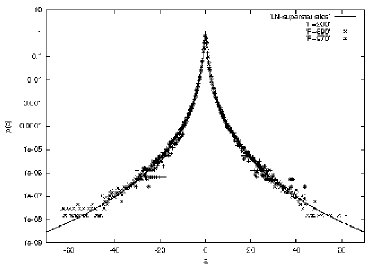
Figure 1: Distribution of acceleration as measured by Bodenschatz boden2 ; boden1 and as predicted by eq. (8), $s^{2}\approx 3$ .

4 Correlations induced by superstatistics

3-dimensional superstatistics induces correlations between the components $a_{x},a_{y},a_{z}$ of the acceleration vector $\vec{a}$. Consider the ratio $R:=p(a_{x},a_{y})/(p(a_{x})p(a_{y}))$. For independent acceleration components this ratio would always be given by $R=1$. However, our 3-d superstatistical model yields the prediction

$$R=\frac{\int_{0}^{\infty}\beta f(\beta)e^{-\frac{1}{2}\beta\tau^{2}(a_{x}^{2}+a_{y}^{2})}d\beta}{\int_{0}^{\infty}\beta^{1/2}f(\beta)e^{-\frac{1}{2}\beta\tau^{2}a_{x}^{2}}d\beta\int_{0}^{\infty}\beta^{1/2}f(\beta)e^{-\frac{1}{2}\beta\tau^{2}a_{y}^{2}}d\beta}.$$ (9)

This is a very general formula, it is also valid for Tsallis statistics, where $f(\beta)$ is the $\chi^{2}$-distribution. Note that $R=1$ for $f(\beta)=\delta(\beta-\beta_{0})$, i.e. if there are no fluctuations in $\beta$ then all components are independent random variables.

Fig. 2 shows $R=p(a_{x},a_{y})/(p(a_{x})p(a_{y}))$ as predicted by lognormal superstatistics.

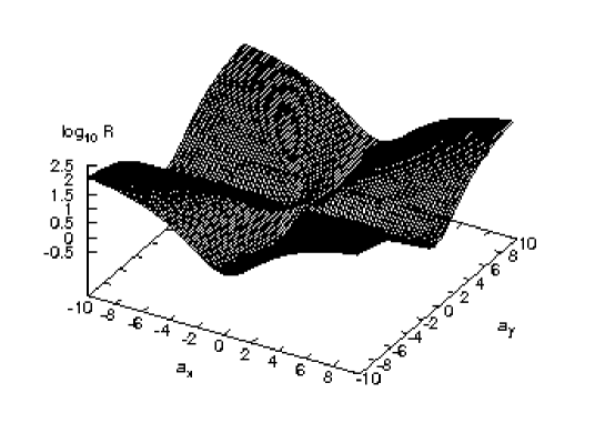
Figure 2: The quantitity $R$ as given by eq. (9) for lognormal superstatistics.

The figure strongly resembles $R$ as experimentally measured by Bodenschatz et al. boden2 in a turbulent flow, see Fig. 3.

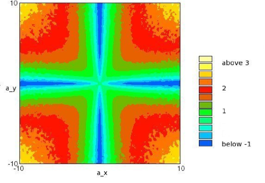
Figure 3: $\log_{10}R$ as measured by Bodenschatz et al. boden2 .

Besides correlations between components one can also look at temporal correlations. The superstatistical model prl2007 allows for the calculation of temporal correlation functions as well. In particular, we may be interested in temporal correlation functions of single components $u_{x}$ of velocity differences, i.e. $C(t)=\langle u_{x}(t^{\prime}+t)u_{x}(t^{\prime})\rangle$. By averaging over the possible random vectors $\vec{n}$ one arrives at the formula

$$C(t)=\frac{1}{3}\langle u_{x}^{2}\rangle e^{-\gamma t}(2\cos Bt+1),$$ (10)

i.e. there is rapid (exponential) decay with a zero-crossing at $t^{*}=\frac{2}{3}\pi B^{-1}$. Exponential decay and zero-crossings are also observed for the experimental data. The model prl2007 also correctly reproduces the experimentally observed fact that the correlation function of the absolute value $|\vec{a}|$ decays very slowly as compared to that of the single components. Moreover, it correctly describes the fact that enstrophy lags behind dissipation zeff .

5 Lagrangian scaling exponents

The moments of velocity differences of a single Lagrangian test particle that is embedded in a turbulent flow scale differently from those measured in a fixed laboratory frame. Our superstatistical model prl2007 allows for the analytic evaluation of the Lagrangian scaling exponents. The moments of velocity difference components $u_{x}$ on a time scale $\tau$ are obtained as

$$\langle u_{x}^{j}\rangle=(j-1)!!m^{-\frac{j}{2}}w^{\frac{1}{8}j^{2}}.$$ (11)

Assuming simple scaling laws of the form $m\sim\tau^{a}$, $w=e^{s^{2}}\sim\tau^{b}$, where $a$ and $b$ are so far arbitrary real numbers, on gets $\langle u_{x}^{j}\rangle\sim\tau^{\zeta_{j}}$ $\sim\tau^{-a\frac{j}{2}+b\frac{1}{8}j^{2}}$. Hence the Lagrangian scaling exponents are given by $\zeta_{j}=-\frac{a}{2}j+\frac{b}{8}j^{2}$. Usually one assumes $\zeta_{2}=1$, hence we get $a=\frac{1}{2}b-1$ thus

$$\zeta_{j}=(\frac{1}{2}+\lambda^{2})j-\frac{1}{2}\lambda^{2}j^{2},$$ (12)

where $\lambda^{2}:=-\frac{1}{4}b$. This prediction is in good agreement with the recent measurements of Bodenschatz et al. boden3 , see Fig. 4.

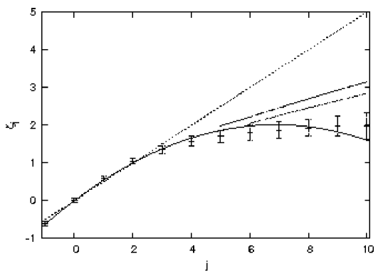
Figure 4: Lagrangian scaling exponents. Data points: Measurements of Bodenschatz et al. boden3 . Solid line: Theoretical prediction of the superstatistical model ($\lambda^{2}=0.085$) prl2007 . Dashed lines: Some other competing models chev .

6 From superstatistics to (generalized) thermodynamics

We end this paper with some more general thoughts. Can we proceed from superstatistics as a merely statistical technique to a proper thermodynamic description? There are some early attempts in this direction by Tsallis and Souza souza . Here we want to follow a somewhat different approach abc : One starts quite generally from two random variables $E$ and $B$ (representing energy and invere temperature) and then considers the following effective entropy for a superstatistical system

$$S[E,B] = S[E|B]+S[B]$$

$$= \int d\beta f(\beta)(\beta U(\beta)+\ln Z(\beta))-\int d\beta f(\beta)\ln f(\beta),$$

where $U$ is the local internal energy and $Z$ the local partition function. One can do thermodynamics with this extended entropy function. It reduces to ordinary thermodynamics for $f(\beta)=\delta(\beta-\beta_{0})$. For sharply peaked distributions $f(\beta)$ this is a slightly deformed thermodynamics, which can be evaluated in a perturbative way. One can also maximize this entropy with respect to appropriate constraints in $\beta$ to get e.g. a lognormal distribution for $f(\beta)$, or generally some other distribution $f(\beta)$ depending on the constraints. For more details, see abc .

7 Summary

• Superstatistics (a ‘statistics of a statistics’) provides a physical reason why more general types of Boltzmann factors (e.g. of power-law type) are relevant for nonequilibrium systems with fluctuations of an intensive parameter.

• There is evidence for three major physically relevant universality classes: $\chi^{2}$-superstatistics $=$ Tsallis statistics, inverse $\chi^{2}$-superstatistics, and lognormal superstatistics. These arise as universal limit statistics for many different complex systems.

• Superstatistical techniques have been successfully applied to a variety of complex systems.

• A superstatistical model of Lagrangian turbulence prl2007 is in excellent agreement with the experimental data for probability densities, correlations between components, decay of correlations, and Lagrangian scaling exponents.

• The long-term aim is to find a good thermodynamic description for general superstatistical systems.

References

- (1) C. Beck, Phys. Rev. Lett. 87, 180601 (2001)
- (2) C. Tsallis, J. Stat. Phys. 52, 479 (1988)
- (3) C. Beck and E.G.D. Cohen, Physica A 322, 267 (2003)
- (4) C. Beck and E.G.D. Cohen, Physica A 344, 393 (2004)
- (5) H. Touchette and C. Beck, Phys. Rev. E 71, 016131 (2005)
- (6) C. Tsallis and A.M.C. Souza, Phys. Rev. E 67, 026106 (2003)
- (7) S. Abe, C. Beck, and E.G.D. Cohen, Phys. Rev. E 76, 031102 (2007)
- (8) P.-H. Chavanis, Physica A 359, 177 (2006)
- (9) C. Vignat, A. Plastino and A.R. Plastino, Nuovo Cimento B 120, 951 (2005)
- (10) G.E. Crooks, Phys. Rev. E 75, 041119 (2007)
- (11) J. Naudts, arXiv:0709.0154
- (12) R.F. Rodriguez and I. Santamaria-Holek, arXiv:0706.0436
- (13) I. Lubashevsky et al., arXiv:0706.0829
- (14) C. Vignat and A. Plastino, arXiv:0706.0151
- (15) A.M. Mathai and H.J. Haubold, Physica A 375, 110 (2007)
- (16) A.Y. Abul-Magd, Physica A 361, 41 (2006)
- (17) S. Abe and S. Thurner, Phys. Rev. E 72, 036102 (2005)
- (18) C. Beck, E.G.D. Cohen, and H.L. Swinney, Phys. Rev. E 72, 026304 (2005)
- (19) C. Beck, Phys. Rev. Lett. 98, 064502 (2007)
- (20) A. Reynolds, Phys. Rev. Lett. 91, 084503 (2003)
- (21) C. Beck, Europhys. Lett. 64, 151 (2003)
- (22) A.M. Reynolds, N. Mordant, A.M. Crawford, and E. Bodenschatz, New Journal of Physics 7, 58 (2005)
- (23) S. Rizzo and A. Rapisarda, Environmental atmospheric at Florence airport, Proceedings of the 8th Experimental Chaos Conference, Florence, AIP Conf. Proc. 742, 176 (2004)
- (24) S. Rizzo and A. Rapisarda, Application of superstatistics to atmospheric turbulence, in Complexity, Metastability and Nonextensivity, eds. C. Beck, G. Benedek, A. Rapisarda, C. Tsallis, World Scientific (2005)
- (25) K. E. Daniels, C. Beck, and E. Bodenschatz, Physica D 193, 208 (2004)
- (26) J.-P. Bouchard and M. Potters, Theory of Financial Risk and Derivative Pricing, Cambridge University Press, Cambridge (2003)
- (27) M. Ausloos and K. Ivanova, Phys. Rev. E 68, 046122 (2003)
- (28) M. Baiesi, M. Paczuski and A.L. Stella, Phys. Rev. Lett. 96, 051103 (2006)
- (29) U. Harder and M. Paczuski, cs/PF/0412027
- (30) C. Beck, Physica A 331, 173 (2004)
- (31) G. Wilk and Z. Wlodarczyk, Phys. Rev. Lett. 84, 2770 (2000)
- (32) G. Wilk and Z. Wlodarczyk, Physica A 376, 279 (2007)
- (33) A. Porporato, G. Vico, and P.A. Fay, Geophys. Res. Lett. 33, L15402 (2006)
- (34) K. Briggs and C. Beck, Physica A 278, 498 (2007)
- (35) A. La Porta, G.A. Voth, A.M. Crawford, J. Alexander, and E. Bodenschatz, Nature 409, 1017 (2001)
- (36) H. Xu, N.T. Ouellette, and E. Bodenschatz, Phys. Rev. Lett. 96, 114503 (2006)
- (37) B. Zeff et al., Nature 421, 146 (2003)
- (38) L. Chevillard et al., Phys. Rev. Lett. 91, 214502 (2003)