A weighted network evolution model based on passenger behavior

Abstract

This paper presents an evolution model of weighted networks in which the structural growth and weight dynamics are driven by human behavior, i.e. passenger route choice behavior. Transportation networks grow due to people’s increasing travel demand and the pattern of growth is determined by their route choice behavior. In airline networks passengers often transfer from a third airport instead of flying directly to the destination, which contributes to the hubs formation and finally the scale-free statistical property. In this model we assume at each time step there emerges a new node with $m$ travel destinations. Then the new node either connects destination directly with the probability $p$ or transfers from a third node with the probability $1-p$. The analytical result shows degree and strength both obey power-law distribution with the exponent between 2.33 and 3 depending on $p$. The weights also obey power-law distribution. The clustering coefficient, degree assortatively coefficient and degree-strength correlation are all dependent on the probability $p$. This model can also be used in social networks.

Most networks in real world are weighted. Recently weighted networks dynamics have attracted much attention. People have developed many new models to understand weighted networks evolution mechanism based on the Barabási-Albert (BA) model 1 which first proposed preferential attachment for networks evolution. Antal-Krapivsky (AK) model 2 relaxes degree preferential attachment to weight driven attachment mechanism. Barrat-Barthélémy-Vespignani (BBV) model 3 ; 4 adds local weight reinforcement dynamics to the structure growth and weight-driven mechanism. Dorogovtsev-Mendes (DM) model gets similar result with BBV model. W. Wang et al6 gives a global weight reinforcement mechanism to structure growth and weight driven attachment to model traffic networks evolution. Guimera and Amaral 7 models world-wide airport networks including spatial information as weight. Researchers begin to put more focus on weight dynamics and weight interaction with other factors Boccalettia .

The above papers all assume the weight changes automatically at each step due to weight and topology coupling mechanism. However this assumption is too rough to understand underlying driving factors and helps little to control and manipulate networks. Transportation networks are good examples to explain this argument. Traffic is composed by passengers who are decision makers. They decide which routes to choose and then changes the traffic on routes. The shortest path finding behavior and congestion phenomenon in networks have been studied by many papers B ; Wu ; Danila ; Danila2 ; Douglas . Passengers collective route selection behavior play a critical role in the hubs formation and the pattern of network growth. For example, in airline industry airline companies provide low price for those who are willing to take transfer flights. Passengers make their decisions based on own time and money consideration. Some sensitive to price select transfer flights and contribute to traffic in hubs. If all passengers are not sensitive and don’t want to transfer, the hubs and thus the popular hub-and-spoke operation model in airline industry since 1970’s cannot come into being. And the world-wide airline networks would not display the structure nowadays. So here we propose a new approach to understand transportation network evolution taking passenger’s route selection behavior into consideration in addition to weight and topology coupling mechanism.

The model assumes at each stage there emerges a new node with $m$ destinations, i.e. new travel demand is created. A passenger who wants to go from origin to destination select his route. He can either fly directly to the destination or transfer at a third place. The probability of taking non-stop flight is $p$ and that of transfer flight is $1-p$. In the transfer case, the passenger determines transfer node based on the weight between transfer node and destination. Analytical results show degree and strength both obey power-law distribution with the exponent between $2.33$ and $3$ depending on $p$. The weights also obey power-law distribution. If $p=1$, the model recover the strength-driven AK model. If we let $1-p=\delta$, it reproduces the results of the BBV model. Simulation confirms the theoretical results. This model is not limited in explaining transportation networks. It can also used to explain social networks which we will discuss later.

The detailed model is described as follows. The initial network has $N_{0}$ nodes with existing links. There are initial weights $w_{0}$ on the links. The networks evolutes according to the following rules:

• Growth. In each step a new node $n$ emerges with $m$ destinations. The probability of one old node $i$ to be the destination is determined by the ratio of its strength $S_{i}$ to the total strength of all nodes:

  $$\pi_{i}=\frac{S_{i}}{\sum_{l}S_{l}}$$ (1)

  which suggests that nodes with large strength have large possibility to be travel destinations.

• Passenger’s route choice. Then the new node $n$ either connects node $i$ with probability $p$ or transfers at a third node $j$ with probability $1-p$. In the former case, a new edge with initial weight $w_{0}$ between $n$ and $i$ is established. In the latter case, things are little complicated. Passengers have to determine which node to choose as the transfer node. They only consider destination’s neighbors which already have links with the destination. The probability of node $j\epsilon\nu(i)$ being chosen as the transfer node is:

  $$\pi_{n-j}=\frac{w_{ij}}{S_{i}}$$ (2)

  Here $\nu(i)$ is the neighbors set of node $i$. $w_{ij}$ is the weight on edge between vertex $i$ and $j$ representing the traffic. Once node $j$ is chosen, a new edge with initial weight $w_{0}$ between vertex $n$ and $j$ is created, and traffic between vertex $i$ and $j$ increases by $w_{0}$. The quantity $w_{0}$ set the scale of weight. We can set $w_{0}=1$ without impact to the model.

With the above two rules, the network grows and stops when nodes reach a preset large number $N$.

The rules has practical implications. In the first rule, a great number of traffic throughput indicate the city is more developed and more attractive to people than those city having little traffic. This rule is identical to those strength-driven models. In the second rule, there are two approaches to get to the destination. If passengers choose transfer mode, they prefer those nodes having frequent flights and large traffic between the destination and transfer node because frequent and large traffic can bring convenience, low price and less waiting time.

Figure 1: Visual description of evolution mechanism. New node $n$ emerges at each step. The old node $i$ becomes travel destination with probability $S_{i}/\sum_{l}S_{l}$. (a) Passengers select one neighbor $j$ of node $i$, to transfer with probability $w_{ij}/{S_{i}}$. The weights update as $w_{ij}=w_{ij}+1$ and $w_{nj}=1$. (b) Passenger go to node $i$ directly creating a new link between $n$ and $i$. The weight $w_{ni}=1$.

This model is also applicable to social networks. For example, in author networks a new researcher is attracted to some famous scientist, but he has no approach to know him directly. Instead he finds that it’s better to know the scientist’s acquaintance with plenty of connections or cooperations between them. With the introduction of that acquaintance, he can finally get to know the scientist. This will also happen in friends networks, actor networks, etc.

To analyze the distribution of degree and strength, we notice the model time is measured by the number of nodes added to the network, i.e., $t=N-N_{0}$. And the natural time scale of the model dynamics is the network size $N$. We treat strength $S$, degree $K$, time $t$ as continuous variables 9 . When a new node $n$ is added into the network, the strength $S_{i}$ of an already present vertex $i$ can increase by 1 if it is selected as a destination or increase by 2 if it is selected as a transfer node. And the degree $K_{i}$ of the vertex $i$ will only increase by $1$ whether it is chosen as destination or transfer node. We have the following equations:

$$\frac{dS_{i}}{dt}=m\frac{S_{i}}{\sum_{l}S_{l}}+(1-p)\sum_{j\epsilon\nu(i)}2m\frac{S_{i}}{\sum_{l}S_{l}}\frac{w_{ij}}{S_{j}}$$ (3)

$$\frac{dK_{i}}{dt}=m\frac{S_{i}}{\sum_{l}S_{l}}$$ (4)

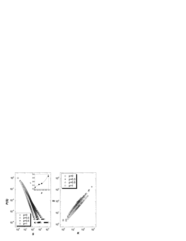
Figure 2: Left: Probability distribution $P(S)$. Data are consistent with a power-law behavior $s^{-r}$. The data are averaged by 20 networks of size $N=10000$ and $m=2$. In the inset, we give the value of $r$ obtained by data fitting together with the analytical expression $r=2+1/(3-2p)$. Right: Correlations between strength and degree. The slopes are all around $1$ indicating linear relationship.

The equation (3) can be rewritten if we notice the sum of strength at large time $t$ is $\sum_{l}S_{l}\approx 2m(p+(1-p)2)t$ and the initial condition $S_{i}(i)=m,K_{i}(i)=m$. So we obtain:

$$\frac{dS_{i}}{dt}=\frac{3-2p}{4-2p}\frac{S_{i}}{t}$$ (5)

$$S_{i}=m(\frac{t}{i})^{\frac{3-2p}{4-2p}},K_{i}=m\frac{S_{i}+2m(1-p)}{3-2p}$$ (6)

The strength and degree of vertices are thus related by a linear equation. It means the model is not only strength-driven but also degree-driven.

From Eq. (6) we get the power-law distribution of the degree and strength $P(K)\sim K^{-r},P(S)\sim S^{-r}$ with the exponent: $r=2+1/(3-2p)=(7-4p)/(3-2p)$. Obviously $r$ is between 2.33 and 3 when $p$ ranges from $0$ to $1$. When $p=1$, passenger always choose connect directly, or in other words there are no transfer behavior. The model is reduced to strength-driven AK model. If we set $1-p=\delta$, the exponent becomes $r=(3+4\delta)/(1+2\delta)$ which reproduces the networks generated by the BBV model. It worths noticing because it indicates that a model based on human behavior can lead to networks produced by automatic topology and weight coupling. $\delta$ in BBV model represents the weight increase in every time period while $1-p$ represents the transfer behavior. The above finding indicates that transfer behavior can induce weight dynamics in BBV model.

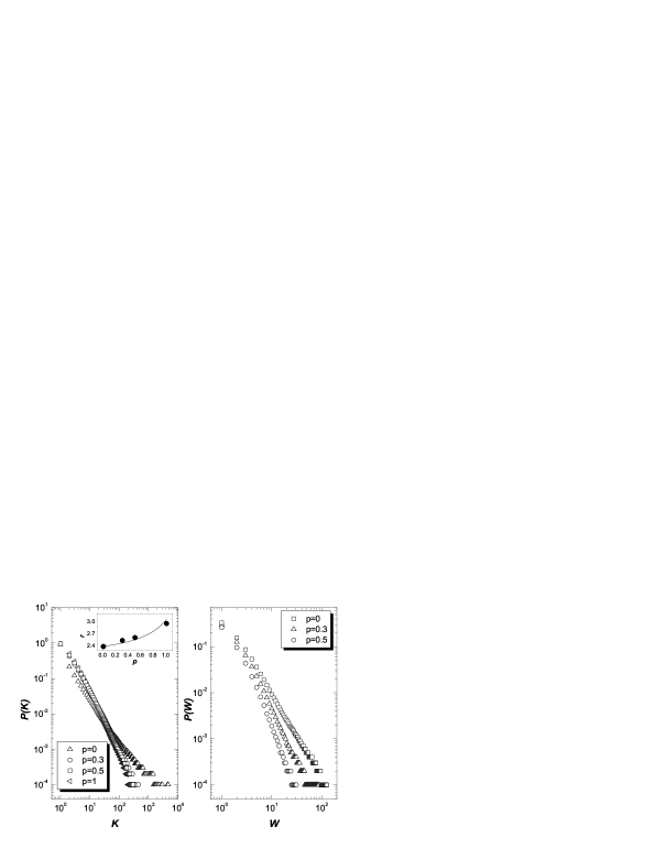
Figure 3: Left: Probability distribution $P(k)$. Data are consistent with a power-law behavior $k^{-r}$. In the inset, we give the value of $r$ obtained by data fitting together with the analytical expression $r=2+1/(3-2p)$. Right: Probability distribution $P(w)$. Data are consistent with a power-law behavior $w^{-a}$. We don’t plot the curve for $p=1$ because in that case all weights are 1 and the distribution cannot be displayed with an infinite exponent. The data are averaged by 20 networks of size $N=10000$ and $m=2$.

The time evolution of the weights $w_{ij}$ can also be computed analytically. Weight $w_{ij}$ between already present node $i$ and $j$ evolves each time either $j$ or $i$ are selected as transfer node to another one. The evolution equation can be written as :

$$\frac{dw_{ij}}{dt}=m(1-p)\left(\frac{S_{i}}{\sum_{l}S_{l}}\frac{w_{ij}}{S_{i}}+\frac{S_{j}}{\sum_{l}S_{l}}\frac{w_{ij}}{S_{j}}\right)$$ (7)

Noticing the initial condition $w_{ij}(t_{ij})=1$ and $\sum_{l}S_{l}\approx 2m(p+(1-p)2)t$, we get

$$w_{ij}=\left(\frac{t}{t_{ij}}\right)^{\frac{1-p}{2-p}}$$ (8)

Thus the weights also have power-law distribution: $P(w)\sim w^{-a}$ with the parameter $a=(3-2p)/(1-p)$. When $p=0$, $a=3$. When the $p\rightarrow 1$, $a\rightarrow\infty$. Actually when $p=1$ there are no transfer behavior and no weight dynamics. All weights are 1. So the probability distribution has an infinite parameter.

In order to check the analytical predictions we performed numerical simulations of networks generated by using the present model with different probability $p$ and network size $N$. The simulation recovers the analytical results. The probability distribution of strength, degree and weight are in good agreement with theoretical predictions. And the strength and degree have linear correlations. When we fit the data, we use the maximum likelihood method to estimate the parameter $r$ 8 . See Fig (2) and Fig (3).

Next we investigate the structural organization of the networks generated by our model by studying correlations of vertices. Using the formula defined by Eq. (4) and Eq. (6) of Ref 4 , we calculate degree-dependent cluster coefficient $C(k)$ and average nearest-neighbor degree $K_{nn}(k)$ (also called degree-degree correlations). They both show disassortative behavior with $C(k)$ and $K_{nn}(k)$ decreasing with $k$, which indicates there are hierarchal structures in the networks. The properties are depending on the parameter $p$. For large $p$, $C(k)$ and $K_{nn}(k)$ are quite flat. While the $p$ decreases, the curves grows.

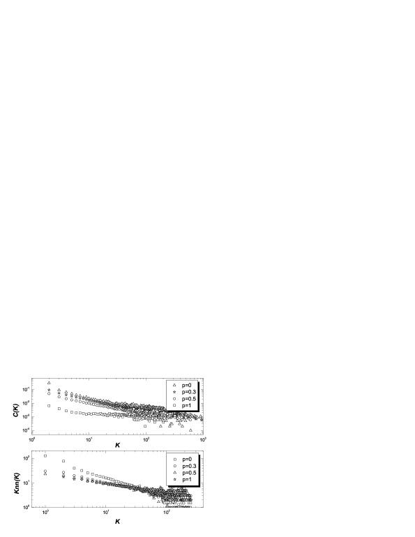
Figure 4: Top: Clustering coefficient $C(k)$ depending on the parameter $p$. Bottom: Average nearest-neighbor degree $K_{nn}(k)$ depending on the parameter $p$. The data are averaged by 20 networks of size $N=10000$ and $m=2$.

This disassortative behavior can be understood in the dynamical growth process. Vertices with large connectivities and strengths are the ones that enter the system early. New vertices are attracted to preexisting vertices with large strengths. In direct connection mode, there builds up a disassortative relation between "old" vertex with high strength and connectivities and "young" vertices with small connectivities. In transfer mode, the transfer vertices also have high connections because it generally is the most weighted in the neighbor of the destination. So there also builds up a disassortative relation between transfer vertices and the new vertices. The average nearest-neighbor degree will be higher than that in direct connection because the transfer mode produces more highly connected vertices than the direct connection mode. The cluster coefficient in transfer mode is larger than that in direct connection mode because transfer mode connects three vertices in one time period thus produces more correlations between vertices. With small $p$ there are more transfer behavior in the networks leading to large $C(k)$ and $K_{nn}(k)$.

In summary we have presented a model for weighted networks evolution that considers human behavior in addition to weight dynamics and topology growth. We investigated the evolution of degree, strength and weight. They are all distributed according to power laws with exponents dependent on the probability $p$ which determines the behavior of passengers. Clustering and correlations between vertices show clear disassortative behavior. The most difference between our model and previous models is that human behavior is incorporated to induce weight dynamics instead of automatic weight dynamics. This reveals the underlying driving force in the growth of transportation networks and social networks. We believe that the model might provide a starting point for the realistic modeling that incorporates human behavior into technological networks modeling.

References

- (1) Barabási A L , Albert R. Science, 286 509-512 (1999).
- (2) T. antal and P. L. Krapivsky, Phys. Rev. E 35, 71, 026103 (2005) .
- (3) A. Barrat, M. Barthélémy, and A. Vespignani, Phys. Rev. Lett. 92, (2004) 228701.
- (4) A. Barrat, M. Barthélémy, and A. Vespignani, Phys. Rev. E 70, 066149 (2004)
- (5) S. N. Dorogovtsev and J. F. F. Mendes, eprint cond-mat/0408343.
- (6) W. Wang, B. Wang, B. Hu, G. Yan, and Q. Ou, Phys. Rev. Lett. 94, 188702 (2005).
- (7) R. Guimera and L.A.N. Amaral, Eur. Phys. J. B 38, 381-385 (2004).
- (8) S. Boccaletti., V. Latora, Y. Moreno, and M. Chavez, D.-U. Hwang, Physics Report, 424 175-308 (2006).
- (9) M. Barthélémy and A. Flammini, eprint physics/0601203v1.
- (10) J. J. Wu, Z. Y. Gao, H. J. Sun, H. J. Huang, Euro physics Letters, 74 (3) 560-566 (2006).
- (11) Bogdan Danila, et al, Physical Review E, 74 046114 (2006).
- (12) Bogdan Danila, et al, Physical Review E, 74 046106, (2006)
- (13) Douglas J. Ashton, Timothy C Jarrett, and Neil F. Johnson, Physical Review letters, 94 058701 (2005).
- (14) R. Pastor-Satorras and A. Vespignani, Evolution and structure of the Internet: A statitical physics approach. (Cambridge University Press, Cambridge, England, 2004).
- (15) A. Clauset, C. R. Shalizi, and M. E. J. Newman, eprint 0706.1062v1.