Charge imbalance and Josephson effects in superconductor-normal metal mesoscopic structures.

Abstract

We consider  a $SBS$ Josephson junction the superconducting electrodes $S$ of which are in contact with normal metal reservoirs ($B$ means a barrier). For temperatures near $T_{c}$ we calculate an effective critical current $I_{c}^{\ast}$ and the resistance of the system at the currents $I<$ $I_{c}^{\ast}$ and $I>>I_{c}^{\ast}$. It is found that the charge imbalance, which arises due to injection of quasiparticles from the $N$ reservoirs into the $S$ wire, affects essentially the characteristics of the structure. The effective critical current $I_{c}^{\ast}$ is always larger than the critical current $I_{c}$ in the absence of the normal reservoirs and increases with decreasing the ratio of the length of the $S$ wire $2L$ to the charge imbalance relaxation length $l_{Q}$. It is shown that a series of peaks arises on the $I-V$ characteristics due to excitation of the Carlson-Goldman collective modes. We find the position of Shapiro steps which deviates from that given by the Josephson relation.

I Introduction

In the theory of the Josephson effect in weak links Josephson it is assumed that the superconducting electrodes are in equilibrium. This means, in particular, that a gauge-invariant potential $\mu$

$$\mu=\frac{1}{2}\partial\chi/\partial t+eV,$$ (1)

is equal to zero Ft1 (we set $\hbar=1$). The Josephson relation follows immediately from this condition

$$2e(V_{2}-V_{1})=\partial\varphi/\partial t,$$ (2)

where $(V_{2}-V_{1})$ is the voltage drop across the Josephson junction and $\varphi=\chi_{1}-\chi_{2}$ is the phase difference. Most works on studies of the Josephson effects were carried out under equilibrium conditions so that the potential $\mu$ is zero in the superconducting electrodes $S_{1,2}$, and Eq. (2) is satisfied Kulik ; Barone . The potential $\mu$ is related to a so called charge imbalance arising due to a different population of the electronlike and holelike branches of the quasiparticle spectrum of a superconductor Ft2 . The conditions under which this charge imbalance may arise were studied experimentally Cl ; Yu ; KlMoi ; Dolan ; VanHar ; Mamin ; Chien ; Strunk and theoretically Rieger ; Tin ; SSJLTP ; AV ; AVUsp ; Ovch .

In the last decade a great progress in preparation of superconductor/normal metal ($S/N$) nanostructures has been achieved. Varies properties of these structures were studied experimentally. One can mention the study of transport Petrashov ; Pothier ; Charlat ; Chien ; Klapwijk ; Shapira and thermoelectric ChandraTherm ; SosninTherm properties, the measurements of the density-of-states EsteveDOS etc. Recently a transition of a thin and short superconducting wire into a resistive state caused by a current $I$ was investigated Bezryadin . In particular, an increase of the critical current $I_{c}$ has been observed when an external magnetic field $H$ is applied Bezryadin . A possible reason for the observed increase of $I_{c}$ may be a polarization of magnetic impurities by the magnetic field $H$ Feigelman ; Bezryadin . Another mechanism has been suggested in Ref.Vodolazov . It has been proposed that an increase of the critical currents characterizing phase-slip centers in a thin $S$ wire may be due to a shortening of the charge imbalance relaxation length $l_{Q}$ under the influence of $H$. However, it remains unclear how this mechanism can work in a pure superconducting state when there is no charge imbalance. As is known (for review see AVUsp ; Rammer ; Kopnin ), the charge imbalance arises only under nonequilibrium conditions. For example, this mechanism may be realized in a superconductor-normal metal ($SN$) nanostructure with a bias current, where the charge imbalance is built up due to injection of quasiparticles into the $S$ wire from the $N$ reservoirs Rieger ; Tin ; SSJLTP ; AV ; AVUsp ; Ovch .

In the present, paper we investigate the Josephson effect in a $NSBSN$ structure under nonequilibrium conditions, in the presence of a bias current $I$ flowing through $SN$ interfaces. In this case the potential $\mu$ arises due to injection of quasiparticles into the superconductors $S$ from the normal reservoirs $N$ ($B$ is a barrier of an arbitrary type). We show that if the length of the $S$ wire $2L$ is less than or comparable with the charge imbalance relaxation length $l_{Q},$ the critical current increases and may significantly exceed the critical current $I_{c}$ in the absence of the normal reservoirs. The resistance of the system also will be calculated for the currents $I\leq I_{c}^{\ast}$ and $I\gg I_{c}^{\ast}$, where $I_{c}^{\ast}$ is an effective critical current. We find the position of Shapiro steps and show that peaks associated with the excitation of collective modes of the Carlson-Goldman type arise on the $I-V$ characteristics.

Note that in recent publications Keizer ; Peeters a $NSN$ system without the Josephson junction was considered and the $I-V$ curve of the system was calculated numerically.

II Model and Basic Equations

We consider the structure shown in Fig.1. We assum that the barrier is located in the middle of the $S$ wire, but the results remains qualitatively unchanged for a system with the barrier located at the $S/N$ interface. The system consists of a superconducting wire ($S$ wire) connecting two normal reservoirs $N$. In the middle of the $S$ wire there is a barrier which provides the Josephson coupling. The transparency of the $SN$ interface is assumed to be high. The analysis can be easily generalized to the case of arbitrary $NS$ interface transparencies. We also assume that the temperature $T$ is close to the critical one $T_{c}$ and therefore the inequality

$$\Delta\ll T$$ (3)

is satisfied ($\Delta$ is the order parameter in the $S$ wire). In this case the effects of the branch imbalance are most significant. The lengths $L$ and $l_{Q}$ are assumed large in comparison with the Ginsburg-Landau correlation length $\xi_{GL}$, i.e.,

$$\xi_{GL}\approx 1.2\sqrt{D/T_{c}}(T_{c}/\Delta)\ll\{L,l_{Q}\},$$ (4)

where $D$ is the diffusion coefficient in the $S$ wire. The charge imbalance relaxation length $l_{Q}$ is determined by inelastic scattering processes and may be rather long (Tin ; SSJLTP ; AV ; Ovch ; AVUsp ). This assumption allows us to consider the order parameter constant in the major part of the $S$ wire. The same limit was considered in Refs. AV ; Ovch where the resistance of the superconductor in a $SN$ system was calculated. The relation between $L$ and $l_{Q}$ may be arbitrary.

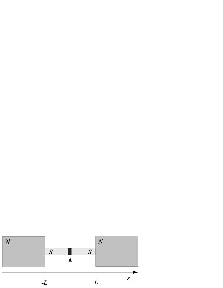
Figure 1: Schematic view of the system under consideration.

Our aim is to obtain a relationship between the current $I$ and the voltage $V_{L}\equiv V(x)$ at $x=L$ (the voltage difference between the $N$ reservoirs is $V_{NN}=-2V_{L}$). We restrict ourselves with voltages $V_{NN}$ small compared to the energy gap $\Delta:$ $eV_{NN}\ll\Delta$. In this limit the distribution function (longitudinal in terms of Ref. SSJLTP ), which determines the order parameter $\Delta,$ is close to the equilibrium one. Another distribution function denoted by $f_{1}$ in Ref. LO (transverse in terms of Ref. SSJLTP ) was found in Ref. SSJLTP ; AV ; Ovch . To be more exact, the so called anomalous Green’s function, $\hat{g}^{(a)}=$ $\hat{g}^{R}\hat{\tau}_{3}f_{1}-f_{1}\hat{\tau}_{3}\hat{g}^{A}$, was found in Refs. AV ; Ovch ; AVUsp , where $\hat{g}^{R(A)}$ are the retarded (advanced) Green’s functions. Using the functions $\hat{g}^{(a)}$ and $\hat{g}^{R(A)}$, one can obtain the expression for the current $I$ in the $S$ wire, which in the main approximation in the parameters $\Delta/T$ and $V/T$ is equal to

$$I=\mathcal{S}\sigma(E+\frac{\pi\Delta^{2}}{2Te}Q),$$ (5)

where $\mathcal{S}$ is the cross section area of the $S$ wire, $\sigma$ is the conductivity of the $S$ wire in the normal state. We assume that the cross section area is small compared to $\{\xi_{GL}^{2},\lambda_{L}^{2}\}$ so that all the vectors $\{\mathbf{I,E,Q}\}$ have only the $x-$component $\{I,E,Q\}$ and depend on $x$. The electric field $E=-\partial V(x)/\partial x$ (we drop the vector potential $A$ because we consider only the longitudinal electric field choosing a corresponding gauge). The condensate momentum $Q$ is defined as

$$Q=(1/2)\partial\chi/\partial x-2\pi A/\Phi_{0}$$ (6)

where $\Phi_{0}=hc/2e$ is the magnetic flux quantum; the vector potential $A$ can be dropped because we do not consider the action of magnetic field. The momentum $Q$ obeys the equation

$$\partial Q/\partial t=eE+\partial\mu/\partial x,$$ (7)

The spatial and temporal variation of the gauge-invariant potential $\mu(x,t)$ is described by the equation AVUsp ; SchoenRev

$$(\partial/\partial t+\gamma)\mu=v_{CG}^{2}\partial Q/\partial x,$$ (8)

where $\gamma$ is a quantity which determines the charge imbalance relaxation rate. It is related to inelastic scattering processes ($\gamma=1/\tau_{\epsilon}$, where $\tau_{\epsilon}$ is the inelastic relaxation time), the condensate momentum ($\gamma\sim DQ^{2}\Delta/T$) in the presence of condensate flow or the gap anisotropy Tin ; SSJLTP ; AV ; Ovch . The velocity $v_{CG}=\sqrt{2D\Delta}$ is the velocity of propagation of the Carlson-Goldman collective mode CG ; SSCollModes ; AVCollModes ; AVUsp ; SchoenRev . In the stationary case Eq.(8) can be written in the form

$$l_{Q}^{-2}\mu=(e/\sigma)\partial j_{S}/\partial x=\partial^{2}\mu/\partial x^{2},$$ (9)

where $j_{S}=\sigma(\pi\Delta^{2}/2Te)Q$ is the density of the supercurrent; $l_{Q}=\sqrt{4TD/(\pi\gamma\Delta)}$ is the penetration depth of the electric field (or the charge relaxation length). Eq.(9) describes the conversion of the quasiparticle and superconducting currents. One can see that the potential $\mu$ arises if the divergence of the supercurrent (or quasiparticle current) differs from zero.

The current in the $S$ wire can also be written as the current through the Josephson junction. In the main approximation it is equal to (see Appendix)

$$I=-\frac{2V_{0}}{R_{B}}+I_{c}\sin\varphi,$$ (10)

where $2V_{0}\equiv 2V(0+)=-2V(0-)$ is the voltage drop across the Josephson junction ($V_{0}$ is negative), $R_{B}$ is the barrier resistance, $I_{c}$ is the Josephson critical current, and $\varphi=\chi(0_{+})-\chi(0_{-})$ is the phase difference. For simplicity we drop here the displacement current $C\partial V_{0}/\partial t$ assuming that the parameter $(CR_{B})e(I_{c}R_{B})$ is small (the main results concerning the critical current and the resistances of the system do not depend on the presence of the displacement current). At $V(L)\ll\Delta$ the critical current equals $I_{c}=\pi\Delta^{2}/4TeR_{B}.$ The first term in Eq.(10) is the quasiparticle current and the second term is the supercurrent.

Eqs.(5-10) describe the system. These equations should be complemented by boundary conditions. Since we consider the voltages smaller than $\Delta$, the distribution function $f_{l},$ which determines the supercurrent, is close to the equilibrium one: $f_{l}=$ $\tanh(\epsilon/2T)$. This implies the conservation of the quasiparticle (correspondingly superconducting) currents at the Josephson junction, i.e.,

$$\mathcal{S}\sigma E(0_{+})=-\frac{2V_{0}}{R_{B}}=I-I_{c}\sin\varphi.$$ (11)

Another boundary condition relates the electric field at the edge of the $S$ wire $E(L)$ to the electric field in the $N$ region $E_{N}$. As is shown in Refs.AV ; Ovch , the electric field $E(x)$ experiences a jump at the $SN$ interface

$$[E]_{SN}\equiv E_{N}-E(L)=rE(L)$$ (12)

where $r\approx 0.7((\Delta/T)l_{\epsilon}/\xi_{GL})^{1/4}\approx 1.17[((T_{c}-T)/T_{c})^{2}\tau_{\epsilon}/\tau]^{1/4}$; $\tau_{\epsilon},\tau$ are the inelastic and elastic scattering times. This jump is small if the temperature $T$ is close to $T_{c}$ and therefore the electric field (accordingly the quasiparticle current) is continuous at the $SN$ interface. For a finite value of $r$ and equal conductivities in the $S$ and $N$ regions we get from Eq.(12)

$$E(L)=E_{N}(1-\frac{r}{1+r})$$ (13)

Here the second term on the right is small near $T_{c}$. Solving Eqs.(5,7,8,10) with the boundary conditions (11-13), we can calculate, in particular, the effective critical current $I_{c}^{\ast}$ and the resistance of the system $R$.

III Resistance and Josephson critical current.

Eqs.(5,7,8,10) are nonlinear equations in partial differentials in which all functions depend on time $t$ and coordinate $x$. Therefore the solution to these equations can not be obtained in a general case. We consider limiting cases of small and large currents $I$.

a) Stationary case; $I<I_{c}^{\ast}.$

If the current does not exceed a critical value $I_{c}^{\ast}$ (the effective critical current $I_{c}^{\ast}$ will be found below), the phase difference $\varphi$ and other quantities do not depend on time. In particular, $\partial Q/\partial t=0$ and the electric field is

$$eE(x)=-\partial\mu/\partial x$$ (14)

The momentum of the condensate is found from Eq.(5)

$$\frac{\pi\Delta^{2}}{2T}Q=eIR_{n}+\partial\mu/\partial x$$ (15)

where $R_{n}=(\mathcal{S}\sigma)^{-1}$ is the resistance of the $S$ wire in the normal state per unit length. The potential $\mu$ is described by Eq.(9). At small currents when the condensate flow does not contribute to the relaxation of the charge imbalance, the length $l_{Q}$ equals: $l_{Q}=\sqrt{4(D\tau_{\epsilon})T/\pi\Delta}$ SSJLTP ; AV ; Ovch . The solution of Eq.(9) is

$$\mu(x)=A\cosh(x/l_{Q})+B\sinh(x/l_{Q})$$ (16)

The electric field and the potential $V(x)$ equal

$$eE(x)=-[A\sinh(x/l_{Q})+B\cosh(x/l_{Q})]/l_{Q},\text{ \ }eV(x)=A\cosh(x/l_{Q})+B\sinh(x/l_{Q})+V_{\ast}$$ (17)

where $V_{\ast}$ is an integration constant.

First we neglect the second term on the right in Eq.(13). From Eqs.(11,13) we find the coefficient $B$ and $A$

$$B=-eR_{Q}(I-I_{c}\sin\varphi),\text{ \ }A=-(eR_{Q}I+BC)/S$$ (18)

where $R_{Q}=l_{Q}/(\mathcal{S}\sigma)$, $C\equiv\cosh\theta$ and $S\equiv\sinh\theta$ with $\theta=L/l_{Q}$.

From Eq.(17) we obtain

$$eV_{L}=eV_{0}+A(C-1)+BS$$ (19)

Writing $V_{0}$ in terms of $B$ (see Eqs.(11,18) ), we can represent $V_{L}$ in the form

$$eV_{L}=B(\frac{b}{2}+\frac{C-1}{S})-IR_{Q}\frac{C-1}{S}$$ (20)

In the stationary case one has $eV_{0}=\mu(0)=A.$ Combining Eqs.(11,18), we obtain from this formula

$$I(\frac{b}{2}+\frac{C-1}{S})=I_{c}(\frac{b}{2}+\frac{C}{S})\sin\varphi$$ (21)

where $b\equiv R_{B}/R_{Q}$. Eq.(21) determines the effective critical current $I_{c}^{\ast}$

$$I_{c}^{\ast}/I_{c}=\frac{bS+2C}{bS+2(C-1)}=\frac{b\tanh(\theta/2)+1+\tanh^{2}(\theta/2)}{\tanh(\theta/2)(b+2\tanh(\theta/2))}$$ (22)

It is seen that the effective critical current $I_{c}^{\ast}$ is always larger than the critical current $I_{c}$ in the absence of the charge imbalance. In the limit of large $b=R_{B}/R_{Q}$ or $\theta=L/l_{Q}$ the effective critical current coincides with $I_{c}$. Therefore in a Josephson junction with a weak coupling between superconductors ($b\gg 1$), the effects of charge imbalance are not important. For a short $S$ wire, we obtain

$$I_{c}^{\ast}/I_{c}=\frac{b\theta+2}{\theta(b+2\theta)}$$ (23)

One can see that $I_{c}^{\ast}$ diverges at $\theta\rightarrow 0$. This fact is in agreement with the results of Ref.Zaitsev , where a very short $NSS^{\prime}$ system was considered, and it was concluded that the stationary state exists at any currents $I.$ However our consideration is valid only for not too small $\theta$ ($\theta=L/l_{Q}\succsim\xi_{GL}/l_{Q}$). The dependence of $I_{c}^{\ast}/I_{c}$ on $\theta$ is shown in Fig.2 for different $b.$

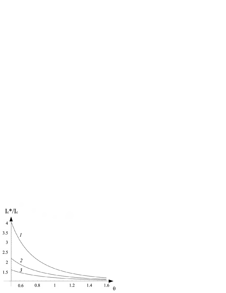
Figure 2: The normalized effective critical current as a function of $\theta=L/l_{Q}$ for $b=R_{B}/R_{Q}$ = 0.2 (curve 1), $b$ = 2 (curve 2), and $b$ = 5 (curve 3)

What is the reason for the increase of the effective critical current from the physical point of view? The critical current is defined as a maximum current $I_{\max}$ at which the stationary state is possible: $\partial\varphi/\partial t=0.$ The current $I_{\max}$ in an ordinary equilibrium Josephson junction coincides with the critical current $I_{c}$ because the first term in Eq.(10) in the stationary state is zero: -$2V_{0}=(\hbar/2e)\partial\varphi/\partial t=0.$ As we noted in the Introduction, this equation follows from the fact that the potential $\mu(x)$ is zero. The same situation takes place near the $S/B/S$ interfaces in a long ($L>>l_{Q}$) $S$ wire. The charge imbalance, which determines $\mu(x)$  arises only in the vicinity of $S/N$ interface and decays on the scale of order $l_{Q}$. Therefore the effective critical current is the maximum current at which the stationary state with nonzero potentials $V$ and $\mu$ is possible. Here we find this current for the case of a short system: $L<<l_{Q}$. Then, the electric field $E(x)$ and potential $V(x)$ can be written as

$$eE(x)\cong-[A(x/l_{Q})+B]/l_{Q},eV(x)\cong A+B(x/l_{Q})\text{ }$$ (24)

The first term in the square brackets of Eq.(24) describes the conversion of the quasiparticle current into the condensate current. In the normal state it is zero because $l_{Q}\rightarrow\infty$.  At $x=L$  the charge is transferred by quasiparticles (we ignore the jump in the electric field setting $r=0$): $S\sigma E(L)=I$. At $x=0$ the quasiparticle current is $S\sigma E(0_{+})=I-I_{c}\sin\varphi.$ Therefore the coefficient $A$ related to the conversion of the quasiparticle current into the condensate one is equal to

$$-A(L/l_{Q})\cong eI_{c}R_{Q}\sin\varphi.\text{ }$$ (25)

On the other hand, at currents $I$ large in comparison with $I_{c}$  one has

$$I\cong-2V_{0}/R_{B}\cong-2A/eR_{B}.$$ (26)

Thus, from Eqs. (25-26), we find the maximum current for the stationary state

$$I_{c}^{\ast}\cong I_{c}(2l_{Q}/bL)$$ (27)

This formula is valid if the ratio $(l_{Q}/bL)$ is large. If the current exceeds this value, the stationary state is not possible. One can say that the length of the S wire is too short to provide the conversion of the quasiparticle current into the condensate current $I_{c}\sin\varphi$.

If we take into account the second term in the boundary condition (13), we obtain for $I_{c}^{\ast}$

$$I_{c}^{\ast}/I_{c}=\frac{2+b\tanh\theta}{\tanh\theta[b+2\tanh(\theta/2)+2r/(S(1+r))]}$$ (28)

The resistance of the system $R_{0}=V_{NN}/I=|2V_{L}|/I$ at $I<I_{c}^{\ast}$ can be easily found with the aid of Eqs. (20,21)

$$R_{0}=2R_{Q}\frac{2\tanh\theta+b}{2+b\tanh\theta}$$ (29)

In limiting cases we find

$$\text{ }R_{0}=2R_{Q}\left\{\begin{array}[]{ll}(2\theta+b)/(2+b\theta),&\theta\ll 1\\ 1,&\theta\gg 1\end{array}\right.$$ (30)

The resistance $R_{0}$ is equal to $R_{B}$ at $\theta\rightarrow 0$ and to $2R_{Q}$ at $\theta\rightarrow\infty$. Thus, the resistance of a short system is a combination of the barrier resistance $R_{B}$ and $R_{Q}$ (the resistance of the $S$ wire near the $SN$ interface). The resistance of a long system equals the resistance of the $S$ wire near the $SN$ interface on the scale $l_{Q}.$ The dependence of the resistance $R_{0}$ on $\theta$ for different $b$ is shown in Fig.3.

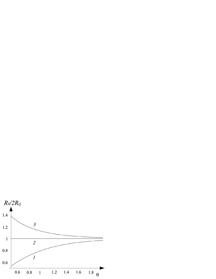
Figure 3: The resistance of the system at currents less than the effective critical current.as a function of $\theta$ for $b$ = 0.2 (curve 1), $b$ = 2 (curve 2), and $b$ = 5 (curve 3)

With account for a finite jump of the electric field at the $SN$ interface (the second term on the right in Eq. (13)), we obtain for $R_{0}$

$$R_{0}=\frac{2}{1+r}R_{Q}\frac{2\tanh\theta+b}{2+b\tanh\theta}$$ (31)

Consider now the case of large currents $I$ when the phase difference $\varphi(t)$ is increasing in time ($\varphi(t)\sim t$) and its oscillating part is small.

a) Quasistationary case; $I\gg I_{c}^{\ast}.$

In this case the condensate momentum is almost time-independent so that $\partial Q/\partial t\cong 0.$ The potentials $\mu,V$ and the electric field $E$ are described by Eqs.(16,17), but the formula for the coefficient $B$ is changed: $B=-eR_{Q}I.$ From Eq.(20) we find the voltage difference between the $N$ reservoirs

$$V_{NN}\equiv-2V_{L}=I[R_{B}+4R_{Q}\frac{C-1}{S}]$$ (32)

and the resistance $R_{\infty}$ at large currents

$$R_{\infty}\equiv[R_{B}+4R_{Q}\tanh(\theta/2)]$$ (33)

In the case of a long $S$ wire ($\theta\gg 1$) we obtain: $R_{\infty}\equiv R_{B}+4R_{Q}$; that is, the resistance of system is the sum of the barrier resistance and the resistance of the regions of the $S$ wire where the electric field penetrates (close to the $SN$ interface and to the barrier). In the case of a short $S$ wire ($\theta\ll 1$) the resistance is: $R_{\infty}\equiv R_{B}+2\theta R_{Q},$ that is, the contribution of the superconducting regions to the resistance decreases.

With account for the second term in Eq.(13) the resistance $R_{\infty}$ acquires the form

$$R_{\infty}\equiv[R_{B}+4R_{Q}(1-\frac{r}{2(1+r)})\tanh(\theta/2)]$$ (34)

That is, the contribution of the $S$ region near the $SN$ interface to the resistance decreases.

IV The I-V characteristics and Shapiro steps

In this Section we analyze the form of the current-voltage (I-V) characteristics and calculate the voltage $V_{Sh}$ which determines the position of the first Shapiro step. At a finite value of the ratio $R_{Q}/R_{B}$ the voltage $V_{Sh}$ differs from that given by Eq.(2). We restrict ourselves with the limit of large currents $I$ employing an expansion in the parameter $I_{c}/I$. In the considered non-stationary case all the quantities depend on time, and in the lowest approximation in the parameter $I_{c}/I$ this dependence is determined by terms of the type $\exp(i\Omega_{J}t)$, where $\Omega_{J}$ is the frequency of the Josephson oscillations. Eqs.(8,9,16,17) can be easily generalized for the non-stationary case. The potential $\mu$ is described again by the equation

$$\partial^{2}\mu/\partial x^{2}=k_{\Omega}^{2}\mu$$ (35)

where $k_{\Omega}^{2}=(i\Omega+\gamma)(i\Omega+\Omega_{\Delta})/v_{CG}^{2}$, $\Omega_{\Delta}=\pi\Delta^{2}/2T$. The solution for this equation is

$$\mu(x)=A_{\Omega}\cosh(k_{\Omega}x)+B_{\Omega}\sinh(k_{\Omega}x)$$ (36)

The electric field and potential have the form

$$eE(x)=-\frac{\Omega_{\Delta}}{i\Omega+\Omega_{\Delta}}\partial\mu/\partial x,\text{ \ }eV(x)=\frac{\Omega_{\Delta}}{i\Omega+\Omega_{\Delta}}\mu+eV_{\ast},$$ (37)

In deriving Eq.(37) we assume that the current $I$ does not depend on time (no external ac signal). From the boundary conditions (11,13) we find

$$B_{\Omega}=-eR_{\Omega}\frac{i\Omega+\Omega_{\Delta}}{\Omega_{\Delta}}(I-I_{c}\sin\varphi),\text{ \ }A_{\Omega}=-(eR_{\Omega}I(1+r)^{-1}+B_{\Omega}C_{\Omega})/S_{\Omega}$$ (38)

where $R_{\Omega}=(k_{\Omega}\sigma)^{-1}$, $C_{\Omega}=\cosh(k_{\Omega}L),$ $S_{\Omega}=\sinh(k_{\Omega}L)$. The electric potential at the $N$ reservoir is

$$eV_{L}=\frac{\Omega_{\Delta}}{i\Omega+\Omega_{\Delta}}[B_{\Omega}(\frac{R_{B}}{2R_{\Omega}}+S_{\Omega})+A_{\Omega}(C_{\Omega}-1)]$$ (39)

Here we took into account the finite value of $r$. The equation for the phase difference $\varphi$ is obtained from the definition of $\mu_{0}=(1/4)\partial\varphi/\partial t+eV_{0}.$ It has the form

$$\frac{1}{2e}(\frac{\partial\varphi}{\partial t})_{\Omega}+[R_{B}+2R_{\Omega}\frac{i\Omega+\Omega_{\Delta}}{\Omega_{\Delta}}\frac{C_{\Omega}}{S_{\Omega}}]I_{c}(\sin\varphi)_{\Omega}=[R_{B}+2R_{Q}(\frac{C_{Q}-1}{S_{Q}}+\frac{r}{(1+r)S_{Q}}]I$$ (40)

We rearrange the terms in Eq.(40) and rewrite it in a dimensionless form

$$(\frac{\partial\varphi}{\partial\tau})_{\omega}=\omega_{J}+[j(1+\frac{2}{b}(\frac{C_{Q}-1}{S_{Q}}+\frac{r}{(1+r)S_{Q}})-\omega_{J}]-[1+\frac{2}{b_{\omega}}\frac{C_{\omega}}{S_{\omega}}\frac{i\omega+\omega_{\Delta}}{\omega_{\Delta}}](\sin\varphi)_{\omega}$$ (41)

where $j=I/I_{c}$, $\omega_{J}=\Omega_{J}/(2eI_{c}R_{B}),$ $\tau=t(2eI_{c}R_{B})$ are the dimensionless current, Josephson frequency and time, respectively; $b_{\omega}=b_{L}\theta_{\omega},$ $b_{L}=b\theta,$ $\theta_{\omega}=\theta_{0}\sqrt{(i\omega+\omega_{\Delta})(i\omega+\omega_{\gamma})}$, $\theta_{0}=(L/v_{CG})(2I_{c}R_{B})\cong 1.11(\Delta/T)^{3/2}\sqrt{T/E_{Th}},$ $E_{Th}=D/L^{2},$ $\omega_{\Delta}=\Omega_{\Delta}/(2eI_{c}R_{B})=1$, $\omega_{\gamma}=\gamma/(2eI_{c}R_{B})$.

The solution is sought in the form $\varphi(\tau)=\varphi_{0}(\tau)+\varphi_{1}(\tau)+...,$ where $\varphi_{n}(\tau)\sim j^{-n}$, for $n\geq 1$. In zero order approximation we obtain from Eq.(41)

$$\varphi_{0}=\omega_{J0}\tau,\text{ }\omega_{J0}=j[1+\frac{2}{b}(\frac{C_{Q}-1}{S_{Q}}+\frac{r}{(1+r)S_{Q}})]$$ (42)

The correction $\varphi_{1}(\tau)$ is equal to

$$\varphi_{1}(\tau)=\omega_{J0}^{-1}[\mathop{Re}\mathcal{L}(\omega)\cos(\omega\tau)-\mathop{\ Im}\mathcal{L}(\omega)\sin(\omega\tau)]$$ (43)

where $\mathcal{L}(\omega)=[1+(2/b_{\omega})(C_{\omega}/S_{\omega})(i\omega+\omega_{\Delta})/\omega_{\Delta}].$

Knowing $\varphi_{1}(\tau)$, one can find a correction to the I-V curve due to the Josephson oscillations. From Eq.(39) we find for the dimensionless voltage drop $<v_{NN}>\equiv-<2V_{L}>/(2I_{c}R_{B})$

$$<v_{NN}>=j[1+\frac{4}{b}(\frac{C_{Q}-1}{S_{Q}}+\frac{r}{2(1+r)S_{Q}})]-[1+\frac{2}{b}\tanh(\theta/2)]<\sin\varphi>$$ (44)

Here $<\sin\varphi>=<\varphi_{1}(\tau)\cos(\omega\tau)>=(2\omega_{J0})^{-1}\mathop{Re}\mathcal{L}(\omega)$. The first term is the Ohm’s law at large currents. The second term is a contribution from the Josephson oscillating current. Therefore the correction to the Ohm’s law is equal to

$$<\delta v_{NN}>=-\frac{1}{2\omega_{J0}}[1+\frac{2}{b}\tanh(\theta/2)]\mathop{Re}\mathcal{L}(\omega)$$ (45)

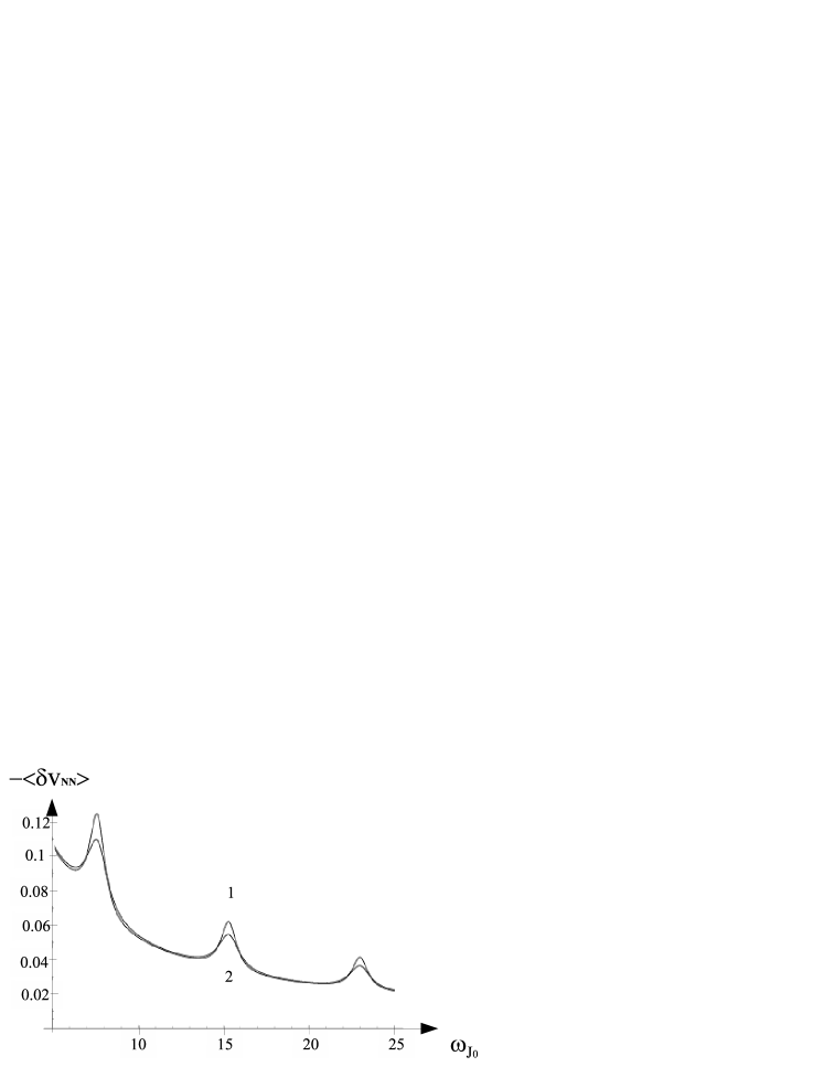
Figure 4: Correction to the I-V characteristics for $\omega_{\gamma}$ = 0.1 (curve 1) and $\omega_{\gamma}$ = 0.5 (curve 2).

In Fig.4 we plot the dependence of this correction $<\delta v_{NN}>$ on the normalized frequency $\omega_{J0}$, which is proportional to the normalized current $j$ (see Eq.(42) ) for two values of damping $\gamma$. In plotting Fig.4 the following values of parameters are taken: $D=50cm^{2}/s$, $T_{c}=1.3K,$ $\Delta/T=0.3$, $b=10,$ $L=0.5mkm$, $\tau_{\epsilon}=2\cdot 10^{-10}s.$ For these values we have: $\omega_{\gamma}=(2eI_{c}R_{B}\tau_{\epsilon})^{-1}=(2/\pi)(\tau_{\epsilon}T)^{-1}(T/\Delta)^{2}\cong 0.27;$ $\theta_{0}=(\pi/2\sqrt{2})(\Delta^{2}/T)L/\sqrt{D\Delta}\cong 1.11(\Delta/T)^{3/2}(T/E_{Th})^{1/2}\cong 0.46,$ $l_{Q}\cong 2mkm$, $\theta=L/l_{Q}\cong 0.25,$ where $E_{Th}=D/L^{2}.$

It is seen that this correction has a series of peaks. These peaks are related to excitation of a collective mode of the Carlson-Goldman type in the system CG ; SSCollModes ; AVCollModes ; AVUsp ; SchoenRev . The excitation occurs if the frequency of the Josephson oscillations $\Omega_{J}=\omega_{J0}(2eI_{c}R_{B})$ coincides with the frequency of the Carlson-Goldman modes $\Omega_{CG}=v_{CG}/L$. In this case the quantity $\mathop{Re}\mathcal{L}(\omega)\sim\tanh^{-1}(k_{\Omega}L)$ has a peak. The possibility to observe such modes in another Josephson system was studied in Ref.AVZ .

Shapiro steps on the I-V characteristics arise if in addition to dc current an ac current flows in the system. In the presence of the ac current, $I_{\sim}(t)=I_{\sim}\sin(\Omega_{ex}t)$, a new term appears on the right in Eq.(40), which is proportional to $I_{\sim}(t)$. The position of the first Shapiro step is determined by the equation Kulik ; Barone

$$\Omega_{J}\equiv(2eI_{c}R_{B})\omega_{J}=\Omega_{ex}$$ (46)

where $\Omega_{J}$ is the frequency of the Josephson oscillations. We obtain the frequency of the Josephson oscillations, $\omega_{J}$, from Eq.(41). At large currents $j$ in the main approximation, $\omega_{J}$ is given by Eq.(42). On the other hand, the normalized voltage $2<v_{NN}>$ corresponding to the same current $j$ can be easily obtained from Eq.(32)

$$2<v_{NN}>=j[1+\frac{2}{b}(\tanh(\theta/2)+\frac{1}{(1+r)S})]$$ (47)

Therefore the deviation of $\ 2<v_{NN}>$ from the value given by the Josephson relation is given by the formula

$$\delta v_{Sh}\equiv\frac{2<v_{NN}>-\omega_{ex}}{\omega_{ex}}\mathbf{=}\frac{2}{(1+r)}\frac{\tanh(\theta/2)-r/S}{b+2[\tanh(\theta/2)+r/((1+r)S)]}$$ (48)

with $\omega_{ex}=\omega_{J0}$. One can see that this deviation can be both negative and positive depending on the parameters $\theta$ and $r$. In the limit of large $b$ the deviation $\delta v_{Sh}=0$, i.e. the Josephson relation is fulfilled. At an arbitrary $b$, the parameter $\delta v_{Sh}$ depends on the quantities $\theta$ and $r$. Thus, by measuring the deviation from the Josephson relation and the resistances $R_{0}$ and $R_{\infty}$, one can determine the ratio $b=R_{B}/R_{Q}$, the parameter $r$ characterizing the jump of the electric field at the $SN$ interface, and the charge relaxation length $l_{Q}=L/\theta.$

V Conclusions

On the basis of a simple model we have analyzed the Josephson effects in a $NSBSN$ nanostructure at temperatures close to $T_{c}$. It turns out that the charge imbalance taking place in this system  essentially changes the characteristics of the Josephson junction. If the barrier resistance $R_{B}$ is not too large in comparison with the resistance of the $S$ wire $R_{Q}$ on the scale of the charge imbalance relaxation length $l_{Q},$ the Josephson critical current increases (see Eq.(23)) and the positions of Shapiro steps deviate from their position in equilibrium Josephson junctions (see Eq.(48)). We have also calculated the resistance of the system for small ($R_{0}$ for $I<I_{c}^{\ast}$) and large ($R_{\infty}$ for $I>>I_{c}^{\ast}$) currents. The ratio of these resistances equals

$$\frac{R_{\infty}}{R_{0}}=\frac{(b+4\tanh(\theta/2))(2+b\tanh\theta)}{2(b+2\tanh\theta)}$$ (49)

Thus, by measuring the ratio $R_{\infty}/R_{0}$ and the deviation $\delta v_{Sh}$, one can determine the coefficient $b$ and the the charge imbalance relaxation length $l_{Q}=L/\theta$.

We have also shown that there is a series of peaks on the $I-V$ characteristics of the system related to excitation of the Carlson-Goldman collective mode. Note that even if the barrier resistance $R_{B}$ is ten times larger than the resistance $R_{Q}$, the peaks in Fig.4 caused by collective mode excitations are clearly visible.

Note that we have adopted several assumptions. One of them is that the voltage $V_{L\text{ }}$ should be smaller than the energy gap $\Delta$. If the voltage is higher than $\Delta$, new effects may arise in the system. In particular, the critical current $I_{c}$ may change sign Klapwijk3 ; VolkovPRL ; Zaikin ; Yip . It would be of interest to measure the $I-V$ characteristics of the considered system in a wide range of the applied voltages.

VI
Acknowledgements

I am grateful to A. Anishchanka for a technical assistance and to M. Kharitonov for bringing Ref.Vodolazov to my attention. I would like to thank SFB 491 for financial support.

VII Appendix

Here we derive the boundary condition (11) and the expression for the current (10). The latter formula in our case is not obvious because the potential $\mu$ differs from zero and the Josephson relation (2) is not valid. Consider the boundary condition at the barrier $B$ for $4\ast 4$ matrix quasiclassical Green’s function $\check{g}$ Zaitsev ; K+L

$$\sigma(\check{g}\partial\check{g}/\partial x)=(2\mathcal{S}R_{B})^{-1}[\check{g}_{0+,}\check{g}_{0-}]$$ (50)

where $\check{g}_{0\pm}=\check{g}(\pm 0)$ are the Green’s functions on the right and left from the barrier $B$. The (11) and (22) elements of the $\check{g}$ matrix are the retarded and advanced Green’s functions $\hat{g}^{R(A)}$ and the (12) element is the Keldysh function $\hat{g}^{K}$. If the voltage in the system $V$ is small in comparison with $\Delta$, the distribution function $f_{l}$ which determines the energy gap $\Delta$ is close to the equilibrium one ($f_{l}\approx\tanh(\epsilon/2T)$).

The current in the system is given by

$$I=\frac{1}{8}\mathcal{S}\sigma\int d\epsilon Tr\{\hat{\tau}_{3}[\hat{g}^{R}(\epsilon,t;r)\partial\hat{g}^{K}(\epsilon,t;r)/\partial x+\hat{g}^{K}(\epsilon,t;r)\partial\hat{g}^{A}(\epsilon,t;r)/\partial x]\}$$ (51)

If we calculate the current with the help of Eqs.(50,51), we obtain Eq.(5). Let us calculate the current through the Josephson junction using the right hand side of Eq.(50). This current consists of three terms: the quasiparticle current $I_{qp}$, the Josephson current $I_{J}$ and the interference current $I_{int}$ Kulik ; Barone . The Josephson current is

$$I_{J}=\frac{\pi iT}{4R_{B}}\sum_{\omega}Tr\{\hat{\tau}_{3}[\hat{f}_{+}\hat{f}_{-}-\hat{f}_{-}\hat{f}_{+}]\}$$ (52)

where $\hat{f}_{\pm}\equiv\hat{f}(\pm 0)=(\hat{\tau}_{2}\cos(\varphi/2)\pm\hat{\tau}_{1}\sin(\varphi/2))\Delta/\sqrt{(\omega_{n}^{2}+\Delta^{2})}$ are the Gor’kov’s quasiclassical Green’s functions on the right (left) from the barrier. Calculating the sum, we obtain

$$I_{J}=I_{c}\sin\varphi$$ (53)

with $I_{c}=\pi\Delta^{2}/4TeR_{B}$. The interference current is given by

$$I_{int}=\frac{\cos\varphi}{16R_{B}}\int d\epsilon(\beta V_{0})(f_{+}^{R}+f_{+}^{A}))(f_{-}^{R}+f_{-}^{A})\cosh^{-2}(\epsilon\beta)$$ (54)

In the main approximation $I_{int}\approx V_{0}\Delta/(4TR_{B})\mathcal{S}\cos\varphi\ln(\Delta/\Gamma),$ where $\Gamma$ is a damping in the spectrum of the superconductor. We see that the interference current is small in comparison with the Josephson current if the voltage $V_{0}$ is smaller than the value $\Delta/\ln(\Delta/\Gamma).$ The quasiparticle current $I_{qp}$ consists of two parts: $I_{qp}=I_{qp}^{(0)}+\delta I_{qp}$, where $I_{qp}^{(0)}$ is determined by the formula

$$I_{qp}^{(0)}=-\frac{1}{8eR_{B}}\int d\epsilon(\beta\partial\chi_{+}/\partial t)(g_{+}^{R}-g_{+}^{A}))(g_{-}^{R}-g_{-}^{A})\cosh^{-2}(\epsilon\beta)=-R_{B}^{-1}(\partial\chi_{+}/\partial t)$$ (55)

The term $\beta\partial\chi_{+}/\partial t\cosh^{-2}(\epsilon\beta)$ is obtained from the equilibrium distribution function after the transformation of the Green’s functions AVUsp : $\check{g}\rightarrow U\check{g}U^{+},$ where $U=\exp(i\hat{\tau}_{3}\chi/2).$ The correction $\delta I_{qp}$ is determined by the response of the system to a perturbation of the potential $\mu$ AVUsp . It is equal to

$$\delta I_{qp}=-\frac{1}{2eR_{B}}\int d\epsilon\frac{\tanh((\epsilon-\Omega/2)\beta)-\tanh((\epsilon+\Omega/2)\beta)}{\Omega}\mu_{0}=\frac{2\mu_{0}}{eR_{B}}$$ (56)

where $\mu_{0}=(1/2)\partial\chi_{0}/\partial t+eV_{0}$. Thus, for the quasiparticle current we obtain the first term in Eq.(10).

The boundary condition (50) may be written for the retarded (advanced) Green’s functions $\hat{g}^{R(A)}.$ Since the distribution function $f_{l}$ approximately coincide with the equilibrium function, one can easily obtain from this boundary condition the equation of continuity of the condensate current at the Josephson junction. Therefore, the quasiparticle current also is continuous at the $SBS$ junction.

References

- (1) B. D. Josephson, Rev. Mod. Phys. 46, 251 (1974).
- (2) Throughout the paper we set .
- (3) I.O. Kulik and I.K. Yanson, Josephson effect in superconducting tunnel structures, Keter Press, Jerusalem (1972).
- (4) A.Barone and G.Paterno, Physics and applications of the Josephson effect, Wiley, NY (1982).
- (5) Note that the charge imbalance is the charge of quasiparticles. This charge is compensated by the charge of the condensate so that the net charge is zero unless we are not interested in small corrections of the order of , where and are the Thomas-Fermi screening length and the length of the electric field penetration into a superconductor.
- (6) J. Clarke, Phys. Rev. Lett. 28, 1363 (1972); J. Clarke and J. L. Paterson, J. Low Temp. Phys. 15, 491 (1974);T. Y. Hsiang and J. Clarke, Phys. Rev. B 21, 945 (1980).
- (7) M. L. Yu and J. E. Mercereau, Phys. Rev. Lett. 28, 1117 (1972).
- (8) T. M. Klapwijk and J. E. Mooij, Physica B 81, 132 (1976).
- (9) G. J. Dolan and L. D. Jackel, Phys. Rev. Lett. 39, 1628 (1979).
- (10) D. J. Van Harlingen, J. Low Temp. Phys. 44, 163 (1981).
- (11) H. J. Mamin, J. Clarke, and D. J. Van Harlingen, Phys. Rev. B 29, 3881 (1984).
- (12) C.-J. Chien and V. Chandrasekhar, Phys. Rev. B 60, 3665 (1999).
- (13) C. Strunk et al., Phys. Rev. B 57, 10854 (1998).
- (14) T. J. Rieger, D. J. Scalapino, and J. E. Mercereau, Phys. Rev. Lett. 27, 1787 (1971).
- (15) M. Tinkham and John Clarke, Phys. Rev. Lett. 28, 1366 (1972); M. Tinkham, Phys. Rev. B 6, 1747 (1972).
- (16) A. Schmid and G. Schoen, J. Low Temp. Phys. 20, 267 (1975).
- (17) S. N. Artemenko and A. F. Volkov, JETP Lett. 21, 313 (1975); Sov. Physics JETP 43, 548 (1976); S. N. Artemenko, A. F. Volkov, and A. V. Zaitsev, J. Low Temp. Phys. 30, 487 (1978).
- (18) Yu. N. Ovchinnikov, J. Low Temp. Phys. 31, 785 (1978).
- (19) S.N. Artemenko and A.F. Volkov, Sov. Phys. Usp. 22, 295 (1980).
- (20) V. T. Petrashov et al., Phys. Rev. Lett. 70, 347 (1993); ibid 74, 5268 (1995).
- (21) H. Pothier et al., Phys. Rev. Lett. 73, 2488 (1994).
- (22) P. Charlat et al., Phys. Rev. Lett. 77, 4950 (1996).
- (23) A. Dimoulas et al., Phys. Rev. Lett. 74, 602 (1995).
- (24) S. Shapira et al., Phys. Rev. Lett. 84, 159 (2000).
- (25) A. Anthore, H. Pothier, and D. Esteve, Phys. Rev. Lett. 90, 127001 (2003).
- (26) A. Parsons, I. A. Sosnin, and V. T. Petrashov, Phys. Rev. B 67, 140502 (2003); ibid G. Srivastava, I. Sosnin, and V. T. Petrashov, 72, 012514 (2005).
- (27) Z. Jiang and V. Chandrasekhar, Phys. Rev. Lett. 94, 147002 (2005); Phys. Rev. B 72, 020502 (2005).
- (28) A. Rogachev, T.-C. Wei, D. Pekker, A. T. Bollinger, P. M. Goldbart, and A. Bezryadin, Phys. Rev. Lett. 97, 137001 (2006).
- (29) M.Yu. Kharitonov and M.V. Feigel’man, JETP Lett., 82, 421 (2005).
- (30) D. Y. Vodolazov, Phys. Rev. B 75, 184517 (2007).
- (31) A.I. Larkin and Yu.N. Ovchinnikov, in Nonequilibrium Superconductivity, edited by D.N. Langenberg and A.I. Larkin (Elsevier, Amsterdam, 1984).
- (32) J. Rammer and H. Smith, Rev. Mod. Phys. 58, 323 (1986).
- (33) N.B. Kopnin, Theory of Nonequilibrium Superconductivity (Clarendon Press, Oxford, 2001).
- (34) R. S. Keizer, M. G. Flokstra, J. Aarts, and T. M. Klapwijk, Phys. Rev. Lett. 96, 147002 (2006).
- (35) D. Y. Vodolazov and F. M. Peeters, Phys. Rev. B 75, 104515 (2007).
- (36) P.L. Carlson and A.M. Goldman, Phys. Rev. Lett. 34, 11 (1975).
- (37) G. Schoen, in Nonequilibrium Superconductivity, edited by D.N. Langenberg and A.I. Larkin (Elsevier, Amsterdam, 1984).
- (38) A. Schmid and G. Schoen, Phys. Rev. Lett. 34, 941 (1975).
- (39) S.N. Artemenko and A.F. Volkov, Sov. Phys. JETP 42, 1130 (1975).
- (40) A.V. Zaitsev, Sov. Phys. JETP 59, 1015 (1984).
- (41) M.Yu. Kupriyanov and V.F. Lukichev, Sov. Phys. JETP 67, 1163 (1988).
- (42) S. N. Artemenko, A. F. Volkov, and A. V. Zaitsev, JETP Lett. 27, 113 (1978).
- (43) J. J. A. Baselmans, A. Morpurgo, B. J. van Wees, and T. M. Klapwijk, Nature 397, 43 (1999).
- (44) A. F. Volkov, Phys. Rev. Lett. 74, 4730 (1995).
- (45) F. K. Wilhelm, G. Schoen, and A. D. Zaikin, Phys. Rev. Lett. 81, 1682 (1998).
- (46) S. K. Yip, Phys. Rev. B 58, 5803 (1998).