Quantized Detector Networks
A review of recent developments

Abstract

QDN (quantized detector networks) is a description of quantum processes in which the principal focus is on observers and their apparatus, rather than on states of SUOs (systems under observation). It is a realization of Heisenberg’s original instrumentalist approach to quantum physics and can deal with time dependent apparatus, multiple observers and inter-frame physics. QDN is most naturally expressed in the mathematical language of quantum computation, a language ideally suited to describe quantum experiments as processes of information exchange between observers and their apparatus. Examples in quantum optics are given, showing how the formalism deals with quantum interference, non-locality and entanglement. Particle decays, relativity and non-linearity in quantum mechanics are discussed.

“ … and all of the apparent quantum properties of light and the existence of photons may be nothing more than the result of matter interacting with matter directly, and according to quantum mechanical laws.”

Feynman’s thesis [1]

This review is divided into four parts. Part $I$ discusses the motivation for the QDN approach to quantum mechanics and covers some relevant historical points. Readers more interested in mathematical details can start with Part $II$, which outlines the formalism. Part $III$ deals with various applications to physics, particularly quantum optics. Part $IV$ is a discussion of some aspects related to the QDN programme.

Throughout this review we use the following acronyms many times: QDN $\equiv$ quantized detector networks, QM $\equiv$ quantum mechanics, SQM $\equiv$ standard quantum mechanics, CM $\equiv$ classical mechanics, SUO $\equiv$ system under observation, ESD $\equiv$ elementary signal detector (or in the case of a source, elementary signal device).

PART I: Motivation

1 Introduction and historical perspective

The landscape of QM is littered with the debris of various interpretations devised to explain away its strange non-classical properties such as wave-particle duality and quantum interference. There is no space to review any of these attempts here. Usually, they failed because their authors tried to view too much of physical reality in terms of familiar classical concepts, such as particles and waves moving about in a background spacetime. Applied to everyday (large-scale) processes, such a strategy usually works well, as evinced by the success of Newtonian and relativistic mechanics, but when it comes to QM, it leads to various traps waiting for the unwary theorist. A notable example is Schrödinger, who originally thought of his quantum waves as smeared out electronic charge, in contrast with the Born probabilistic interpretation [2, 3] generally accepted today.

Classical thinking in QM persists to this day in one form or another, ranging from attempts to split electrons [4] to paradigms such as the Multiverse [5] and decoherence [6], which in their original formulations were based on the assertion that the Schrödinger equation alone suffices to explain all of physics. Such schools of thought view the quantum wavefunction as a fundamental object in its own right. In this article we will emphasize the point that even to talk casually about an “electron wavefunction”, as is commonplace amongst quantum theorists, is to risk applying classical thinking inappropriately to quantum physics. Our view is that a quantum wavefunction is contextual, i.e., without reference to any observer and their apparatus, such a wavefunction is a physically meaningless concept.

Our aim in QDN is to eliminate as far as possible concepts which are inessential, potentially misleading, or simply metaphysical (i.e., incapable of verification). Some mathematical concepts such as labstates and Hilbert spaces are used heavily, but in such cases, the motivation for them stems from a desire to avoid mental imagery as much as possible. The most important guiding principle has been to ask what exactly do experimentalists do when they perform quantum physics experiments, and then model the answer to that question according to established quantum mechanical principles.

2 The importance of observers and their apparatus

Any reasonable interpretation of QM should involve at least a rudimentary recognition and understanding of the roles of the observer and their apparatus in a quantum experiment. To understand what QDN says on this, consider the analogy with cinematography. As we watch a film, we generally tend not to think about the camera or the film crew who made the film. If we did, not only would that spoil the film, but we would be acknowledging the fact that the film could not have been made without the camera. We would be reminded too of the unfortunate fact that the presence of film crews at actual events such as riots often influences those events, and indeed, without the presence of the film crew, those events might never have taken place at all. The best films are those in which the presence of the camera gets overlooked in the mind of the viewer, so that they are deceived into believing that what is seen on screen is independent of the process of observation, and is somehow real on that account. This is a classical world view of reality.

Problems arise when viewers start to interpret a film, which is just a representation of reality, as being that reality itself. Likewise, problems arise in SQM when physical reality is thought as a wave-function. QDN regards QM as the correct set of rules governing information exchange between apparatus and observer, rather than any commentary on the nature of reality. If the only things observers can ever deal with are signals from their apparatus, then nothing need be said beyond that, and so QDN does not comment on the existence or otherwise of SUOs.

3 Origins of QDN

Although many of the core principles of QDN had been developed earlier [7, 8, 9], the catalyst for the development of QDN in the form described here was a reading of Harry Paul’s book on quantum optics [10]. That book emphasizes the essential non-classical properties of the photon concept, making it clear via numerous discussions of actual (as opposed to imagined) laboratory experiments that photons cannot be “particles” in the sense of a cricket ball or baseball. What impressed us most were Paul’s accounts of situations where a photon appears to originate from several correlated sources. We found ourselves trying to understand those experiments in terms of what the observers were doing with their apparatus, rather than in terms of the conventional quantum optics formalism, which uses photon creation and annihilation operators. We asked the question: if photons are not actually “there” as particles per se, then what precisely does it mean to represent them by particle-like creation and annihilation operators? The result was “quantum register physics” [11, 12], which evolved into QDN in the form described here.

Perhaps the best way to understand the core principles of QDN is to see them as equivalent to the principles which motivated Heisenberg’s approach to QM [13]. This is now known as matrix mechanics, because the noncommuting variables Heisenberg introduced could be regarded as transition matrices. This allowed Schrödinger to demonstrate the mathematical equivalence of his wave mechanical approach to QM to the algebraic approach of Heisenberg [14]. However, the underlying principles on which Heisenberg based his work were radically different to those motivating Schrödinger. It seems quite wrong to equate the two formulations of quantum mechanics simply because the mathematics of one can be transformed into the mathematics of the other.

Certainly, Heisenberg himself did not like the visual imagery associated with Schrödinger’s equation. Scientific theories are not just sets of mathematical rules for making predictions, but also require specific ways of thinking about physical situations. Sometimes, these lead to paradigms which are unphysical dead-ends, such as the use of epicycles to describe the motion of planets, the phlogiston theory of heat and the aether concept in Maxwellian electrodynamics. Heisenberg’s crucial idea was to focus only on those aspects of an experiment which are accessible to observation. This seems to be a position sufficiently far from metaphysics as to merit the status of a central principle in physics, and we have tried to respect it as much as possible in our development of QDN.

Not many scientists appeared to follow Heisenberg footsteps, the majority preferring Schrödinger’s wave mechanical approach. A notable exception was Feynman, who attempted to avoid using the electromagnetic field in a novel formulation of electrodynamics [1]. Despite his recorded disdain for the philosophy of science and his success in developing practical calculational methodologies in SQM, he was not entirely disinterested in quantum philosophy (i.e., thinking about what QM means). It led him to think of photons as something to do with apparatus, as the quote from his thesis, given at the start of this review, expresses in a succinct way. We shall return to his ideas presently.

To give some balance in this review of QDN, we point out some of the issues it does not explain at this time. It does not “explain away” intrinsic quantum phenomena such as outcome randomness and interference, but this is true also of SQM. An important currently unresolved issue awaiting our attention is a QDN description of SUOs conventionally described via continuous degrees of freedom. For example, we have not yet developed a QDN approach to the calculation of atomic energy levels, something which the Schrödinger equation does with relative ease. However, that was a problem with Heisenberg’s matrix mechanics also, and in this respect QDN is no different. It is possible QDN will not turn out to be a good approach for those sorts of calculations. Our experience with algebraic approaches to QM such as infinite component wavefunctions leads us to the expectation that the issue will be resolved satisfactorily in due course. The harmonic oscillator, for example, can be described as well via a purely algebraic formulation as it can via a purely wave mechanical approach, and this makes a QDN description of that system relatively easy to develop [15, 16].

On the positive side, apart from giving a novel perspective on physical reality, QDN gives a useful computational methodology readily applicable to certain branches of quantum optics. In particular, the formalism is closely allied to quantum computation, which gives it a modern flavour. It should be possible to encode QDN in computer algebra packages, thereby opening the door to the efficient calculation of quantum amplitudes for the outcomes of quantum optics experiments of arbitrary complexity.

4 Why CM appears to work

Before $1900$, there were very few indications that there was anything wrong with CM, the Rayleigh-Jeans ultraviolet catastrophe and the classically unaccountable stability of matter being perhaps the most important of these. CM works as well as it does because of a number of interlinked factors working together. It is important to understand these factors, because they have played important roles in the development of CM and QM.

First, there is the crucial role of technology. QM was discovered and formulated only after certain advances in technology had been made, particularly in spectroscopy. Without these advances, the flaws in CM would have remained hidden, the relatively small size of Planck’s constant being a major contributor to this.

A second factor is that objects in the real world generally involve extremely large numbers of degrees of freedom, which tend to behave collectively as if the principles of CM were valid. QM experiments are generally characterized by the careful way in which environmental factors are excluded or controlled so as to allow focus on only a very few specially selected degrees of freedom, such as electron spin. Good examples are double-slit experiments in quantum optics, the Stern-Gerlach experiment, and high energy particle scattering experiments. It is only under the most carefully controlled conditions that quantum processes reveal their spectacular non-classical properties clearly.

A third factor is the relative persistence in time of many structures or patterns in the environment, compared with the timescales typical of quantum experiments. This, coupled with the tendency of the human brain to objectify complex phenomena, particularly when they re-occur with predictable and well-defined characteristics, leads to a mental image of the universe as divided into separate objects, such as observers, apparatus, and SUOs.

These images have limitations and can break down spectacularly in the quantum domain. For example, electrons are generally regarded as point-like objects with a well-defined mass, because in many experiments, that is a good approximation. However, from the point of view of quantum field theory, any charged particle is surrounded by a cloud of virtual photons which is constantly interacting with its environment at long range. In consequence, the full electron propagator has a cut rather than a simple pole, which means that electron mass is contextual, i.e., depends on what is being measured and how. Another example is the simplest atomic system, hydrogen, which is far from being just an electron bound to a proton.

5 The road to QM

The first real crack in the classical world view of reality came in $1900$ with Planck’s paper on the quantization of energy [17]. An important fact about Planck’s paper is that he did not propose that the electromagnetic radiation field itself contains quanta of energy. Planck referred only to the behaviour of atomic oscillators absorbing and emitting radiation, which they were postulated to do in a discrete way. If we take the liberty of regarding atoms as detectors of radiation rather than being SUOs themselves, then it seems not unreasonable to interpret Planck’s article as the first real paper on an instrumentalist approach to QM. Planck’s idea is at odds with CM because it is difficult if not impossible to reconcile his vision of discrete energy levels in atomic oscillators with the assumed existence of continuous Maxwellian electromagnetic fields propagating between those atoms.

The crack opened wider when Bohr published his model of the hydrogen atom in $1913$ [18]. From the perspective of CM, this model is a mass of inconsistencies and contradictions like Planck’s idea; the classical electron is assumed to be held in its atomic orbit by classical forces but is not permitted to spiral into the nucleus under the effects of the inevitable radiation damping predicted by Maxwellian electrodynamics. It is simply impossible to understand how discrete energy levels could occur and persist if the electromagnetic field is described in terms of the continuum dynamics equations of Maxwell. However, as with Planck’s idea discussed above, we can rationalize Bohr’s model to some extent if we interpret his atoms as being part of the detecting apparatus and not SUOs.

By interpreting their work in this way, the “old quantum mechanics” (OQM) of Planck, Bohr and Sommerfeld may be regarded not as a collection of ad hoc ideas swept aside by the sudden discovery of wave mechanics by Schrödinger in $1926$, but as important steps in the development of a new approach to observation. The culmination of that development was Heisenberg’s seminal paper [13] in $1925$ of what subsequently became known as matrix mechanics.

6 Heisenberg’s core philosophy

Heisenberg had been a student of Sommerfeld’s and contributed to OQM. He came to the conclusion that the principles of CM were incorrect and discovered how to remedy the situation. His vision about reality was remarkably consistent and clear in the years $1925-27$. Above all, it was radical, with extremely deep implications. What he wrote about electron trajectories remains very disturbing, presenting a picture of a reality which has no existence or meaning other than through the processes of observation. In his ground-breaking $1927$ paper on the uncertainty principle [19] he wrote: “I believe that one can fruitfully formulate the origin of the classical ‘orbit’ in this way: the ‘orbit’ comes into being only when we observe it.” This is a complete rejection of CM principles.

Although Heisenberg’s matrix mechanics was accepted at the time, his core philosophy did not take hold generally and his algebraic formalism was soon overwhelmed by Schrödinger’s wave mechanical approach. Moreover, it had to contend with Einstein’s approach to physics, which in contrast is quite classical. Einstein remained to the end of his days a leading supporter of the classical world view. In $1905$ he published his famous papers on special relativity (SR) and on the photo-electric effect. Although conventional wisdom suggests that these papers overthrew classical principles, we argue that they actually reinforced their core values, because the imagery is entirely classical.

The fact is, SR is not a theory that describes observer-SUO dynamics, but a comparison of different observers’ accounts of the same SUO, given that each observer sees it classically. This assumes that extraction of information about an SUO can come cost free to both observer and SUO. SR in its traditional formulation simply does not incorporate the fundamental quantum principle that an act of observation (i.e., any process which extracts information) necessarily changes the state of an SUO.

To illustrate the pitfalls when QM is mixed with relativity, consider a single photon. Not only does SR allow us to talk of such a thing as an object in its own right, but actually gives the Doppler shift between the two frequencies associated with that photon as seen by two different, relatively moving observers. The problem is that in reality, a single photon can be observed by one observer only. What is meaningful is a comparison of what each observer would have seen if they had in fact been the one who had observed the photon. This touches on the logical-philosophical notion of counterfactuality. Counterfactuality, or discussion of might-have-beens and what-ifs, is a safe exercise in a world run on classical principles, but a dangerous one when quantum processes are involved.

A committed relativist’s counter-argument to our concerns would be that a proper SQM discussion of a single photon should really be a statistical one, i.e., given in terms of ensembles, and that Doppler shifts and suchlike should only be inferred from that form of discussion. This would be in fact an argument in our favour, because it demonstrates that the conventional formulation of SR, which makes no reference to ensembles or statistical principles, is too simplistic and takes no account of what really goes on during a quantum experiment.

As for the photoelectric effect, Einstein’s vision of quanta residing in the electromagnetic field is a clear attempt to maintain a classical world view. It represents a move away from what Planck wrote about, i.e., the atomic oscillators, towards a perceived SUO, the electromagnetic field, the properties of which it is assumed are being studied. It should be admitted that there is room for the SUO concept, when it works and does not mislead, and it is undeniable that Einstein’s papers had enormous impact on subsequent physics. However, that does not mean that the ideas in those papers represent the actual quantum physics of the process of observation in an adequate way.

An indication of how hard it was for Heisenberg’s ideas to be accepted was the speed with which his approach was abandoned once Schrödinger published his papers on wave mechanics in $1926$. This was partly due to the much better and well-known computational technology associated with wave-mechanical linear differential equations, in contrast to the generally intractable nonlinear algebraic formalism introduced by Heisenberg. An equally important factor was the ease with which waves can be visualized in the mind’s eye. Visualization of objects or waves in space is an important feature in CM, so to people thoroughly conditioned to that way of thinking, Heisenberg’s abstract approach would inevitably appear intangible and perhaps absurd.

It was Max Born, mentor and collaborator of Heisenberg’s, who played the principal role in destroying the classical interpretation of Schrödinger’s waves by interpreting them in terms of probability [2]. As with most historical matters, things are rarely as clear-cut as tradition and conventional wisdom suggest. According to Born’s Nobel lecture [3], it was Einstein himself who motivated him at a crucial stage to develop the statistical interpretation of the wave-function.

As an aside, towards the end of his Nobel lecture, Born stated that he believed in particles, but qualified this with the view that “Every object that we perceive appears in innumerable aspects. The concept of the object is the invariant of all these aspects.” This is equivalent to the position taken in QDN: the particle concept is a resumé of certain consistent patterns of behaviour in our observations.

Few theorists followed Heisenberg’s specific philosophical path after $1926$. An important exception was Feynman, who whilst still a student, began to think about photons as a manifestation of the properties of apparatus, rather than as intrinsic “things” in their own right. His ideas are well expressed in the quotation given at the start of this review [1]. The objective of his doctoral thesis was to describe the interaction of particles, such as electrons, without the intervening fields (the electromagnetic field in the case of electrons). In this he was only partially successful and subsequently recanted his views, once the QED calculation of vacuum polarization had turned out to be so successful. Before that happened, however, he had developed the path integral formulation of quantum mechanics, with deep and lasting consequences for modern physics. We shall show that QDN is fully consistent with Feynman’s path integral formulation.

It is worth trying to identify the reason for Feynman’s (albeit limited) success in his instrumentalist programme. Although quantum field theory treats all fields in a democratic fashion, it does not ignore their individual properties. Electrons are fermions, whereas photons are bosons. This is a difference that gives electrons more of a permanence, or identity, than photons. There is no theorem which requires photon number to be conserved, whereas total electric charge is conserved in any interaction. Provided electron-positron pair production thresholds are not exceeded, then it can be meaningful to think of interacting electrons as having an identity during that interaction. Under those circumstances, they can be regarded as part of the detecting equipment involved in an experiment. For example, in any Feynman diagram involving in and out electron propagator lines which do not run back in time, such as in Compton scattering, we can think of each fermion line as the worldline of a detector which responds to electromagnetic exchanges with other such detectors. Feynman’s aim in his thesis of eliminating the intervening photons can be seen in this light as an instrumentalist approach to QM.

7 The role of physical space

The idea that physical space is a three-dimensional manifold with a metric is such a central concept in CM and SQM that it is necessary to comment on it here, because QDN regards it quite differently. In QDN, physical space is regarded as contextual, i.e., manifests itself differently according to the details of an experiment. There are some experiments, such as those in quantum optics described later on in this review, where physical space is frequently a secondary, or even irrelevant, factor. The idea that physical space is a pre-existing manifold with a metric over which physical phenomena act out their dynamics is neither correct nor incorrect, but useful insofar as the experimental context justifies it. Certainly, we find it hard to describe the structure of real apparatus without invoking physical space, but we have to question the need to believe in SUOs moving around it, particularly in the case of photons and other elementary particles. Wave-particle duality in SQM is a manifestation of something not quite correct with such a belief.

A particular difficulty in explaining the QDN perspective on space is not that it is wrong, but that all the evidence from the world around us seems to contradict it. A typical objection, for example, would be that when astronomers observe stars, these appear to have all the characteristics of objects at great distances from the observers. Distant stellar images are reduced in angular size and in intensity exactly as predicted by the traditional model of space as a three-dimensional continuum.

There are several arguments against this sort of objection. First, astronomers do not observe stars just like that, but are themselves embedded in a vast amount of contextuality, preserved and carried forwards in time by the phenomenon of persistence (mentioned above), and much of this is well modelled using the physical space concept. Astronomers know they live on a planet which is in a solar system, which is itself part of a vast galaxy, and so on. All of this contextuality is an essential ingredient in the interpretation of stellar observations. Because of the absence of such contextual information, ancient astronomers made numerous stellar observations but could not deduce our conventional spacetime model of the universe. In consequence, their models of the universe were often quite bizarre by modern standards.

A second argument concerns the observations themselves. Astronomers build up pictures based on physical space only after large numbers of photons have been captured from stellar sources. A single photon captured by a detector gives no information by itself as to the nature of the source of that photon, not even as to whether there has been a Doppler shift, or at what distance the source is situated. The space concept is of limited value in this case. At best, some information may be acquired about the approximate direction of the source, but this requires some specific knowledge about the apparatus, such as where it is pointing. This supports the QDN view that contextual knowledge about apparatus is an essential ingredient in the interpretation of observations.

A third argument concerns the Born interpretation of wave-functions and wave-particle duality. It seems impossible to reconcile the classical notion of an electromagnetic wave radiating from a star with single photon capture a long way away from that star. Electromagnetic waves are best regarded as probability amplitude waves, not as swarms of photons. Any attempt to view quantum wave-functions in objective terms, such as in Bohmian mechanics [20], encounters great difficulties in reconciling spherically symmetric wave propagation with the wave-function collapse associated with single photon capture.

A fourth argument is that the numerous non-local correlation effects which have been empirically confirmed to date demonstrate that distance seems to have no significance as far as certain forms of quantum information are concerned.

The QDN view of physical space lies at the core of its instrumentalist philosophy. As with Heisenberg’s matrix mechanics, this does not make it easy to accept on an intuitive level, but that does not invalidate it. A useful way to think about quantum experiments is to imagine the observer from the position of a blind and deaf person receiving occasional discrete tactile signals from their immediate surroundings, rather than from the perspective of a viewer swamped by a continuum of audio-visual signals appearing to come from all around them. If the QDN perspective on physical space is correct, then one implication is that conventional approaches to “quantum gravity” should fail in the long run, because they generally assume space to be some sort of continuous SUO which needs to be quantized. The programme of quantum gravity might be as futile as attempts to quantize the classical continuum equations of fluid mechanics.

This concludes our historically flavoured motivation for QDN. In the next part, we discuss the mathematics of our approach. It will be seen that Heisenberg’s original ideas can be encoded into a general mathematical formalism virtually identical to that used in quantum computation.

PART II: Formalism

8 Elementary signal detectors and signal bits

Elementary signal detectors (ESDs) are central to QDN. An ESD is any physical device or procedure permitting an observer to extract classical elementary yes/no information from it at a given time. This information is an answer to the basic question: “is there a signal in this detector or not?”.

An ESD need not be located in physical space at a specific place. In practice, some degree of localization will be involved, because physics laboratories tend to be localized in space and time. The information carried by a signal from an ESD need not represent a localized quantity such as position, either. ESDs are used in QDN to model quantum outcomes of experiments, and are analogous to projection operators in SQM, with some important differences.

QDN assumes that all measurements in physics can be described in terms of amplifications of quantum signals from collections of ESDs, to such levels that observers in laboratories can interrogate their apparatus in a classical way. What this means is that an observer can always determine a yes/no answer unambiguously from an ESD, if they choose to look. Underneath this classical veneer, however, there exists the quantum domain where ESDs operate according to the basic quantum rules described in this review. How signal amplification occurs is of course important, but beyond the scope of this particular review.

An objection to these ideas, coming from experimentalists, would be that they do not do physics in such a way. In fact, careful examination invariably shows that they do. Ultimately, everything experimentalists see, record and interpret is expressible in terms of vast but finite numbers of yes/no answers to basic questions. For example, when an experimentalist gives the $x-y$ coordinates of a black spot on an otherwise white screen, those two numbers represent a really economical way of summarizing a vast amount of discrete information, most of it contextual and arising from the initial set-up of the apparatus. These two numbers are a concise way of saying that the answer to the basic question is this spot black? is no for every one of the countless spots on the screen, except for just one of them, for which the answer is yes.

Experimentalist may report their results in terms of real numbers, but in reality all they are dealing with are good discrete approximations to an imagined continuous reality. QDN cannot concede any argument on this point, precisely because its goal is to model reality as it is experienced, not as it is imagined to be. On this account, experimentalists should try to avoid expressions such as “We found the position of the particle to be here”, because the associated imagery can be misleading. Ideally, they should simply say what sort of signals they have observed in their apparatus, and leave any interpretation as to what those signals mean to theorists.

To illustrate the difference between how SQM and QDN model quantum outcomes, consider an idealized Stern-Gerlach experiment, illustrated in Figure $1$. In such an experiment, it would be found that when an electron had passed through the strong inhomogeneous magnetic field in the middle of the device, there would be two distinct regions or spots on the detector screen where it could land and be detected. Each electron passing through the apparatus would land on only one of these sites each time. Which site was landed on could not be predicted in advance in general (this depends on the way the electron was prepared), but a consistent probability distribution would be built up after sufficient runs of the experiment had taken place.

The SQM formalism assigns a ket vector $|$up$\rangle$ to the state of those electrons which had landed on one particular spot, and a ket vector $|$down$\rangle$ to the state of those which had landed on the other spot. These two vectors are then assumed to form an orthonormal basis set for a two-dimensional Hilbert space called a quantum bit, or qubit.

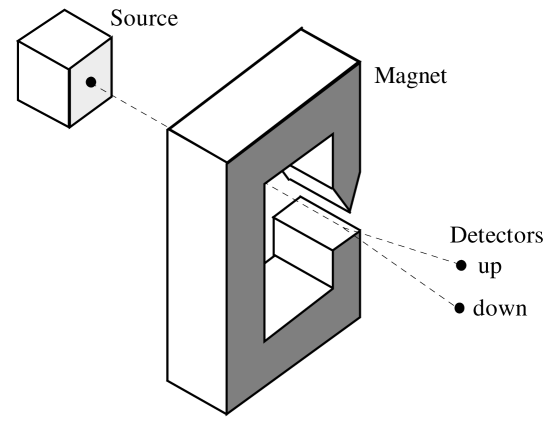
Figure 1: The Stern-Gerlach experiment.

SQM assumes that each time a single electron passes through the apparatus, only one outcome signal is generated, either at the up spot or else at the down spot. The physical justification for this assumption stems from the law of electric charge conservation, which has never been observed to be violated, and from the fact that electrons cannot be split into fractionally charged objects.

Whilst SQM takes a minimalist approach to the modelling of outcomes, QDN appears to go the other way and allows for other logical possibilities to exist in principle. For example, suppose the observer knew that a single electron had been sent into the device. Without knowing in advance the details of the apparatus, it is logically possible to imagine that when the up and down sites were looked at separately, no electron signal would be seen at either, indicating a net loss of electric charge. Another logical possibility is that an electron signal would be found at each of them, suggesting a total of two electrons had emerged.

The use of electric charge conservation to rule out each of these exotic possibilities in SQM is specific to the details of the experiment; it could not be applied for example in the case of electrically neutral particles such as neutrons. It is in fact possible to do analogous non-linear optics experiments with photons where such exotic outcomes could occur. In spontaneous parametric down-conversion for example, a single incoming photon could stimulate a crystal in a device to emit two photons, each of which could be detected at a different site, giving rise to a total of two signals.

Once such logical possibilities are taken into account, it becomes clear that the important factor determining which signals could actually be observed is the physics of the apparatus. It is the apparatus which determines the dynamical possibilities of signal outcomes; if the apparatus is changed then the dynamics changes, and that in turn generates different signal possibilities.

According to QDN principles, the basic signal question should be asked of each ESD available to the observer at the same time, independently and irrespective of any answer obtained from any other ESD at that time. This is not what happens in the SQM approach to the Stern-Gerlach experiment, where an examination of either one of the two outcome spots is assumed to imply the signal state at the other. QDN represents the two possible outcomes of the Stern-Gerlach experiment by two separate qubits $\mathcal{Q}^{1}$ and $\mathcal{Q}^{2}$, as shown in figure $2$, rather than the one qubit used in SQM.

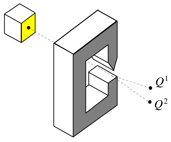
Figure 2: Qubit assignment for the Stern-Gerlach experiment.

More generally, a quantum experiment with $k$ outcomes is described in QDN by $k$ ESD qubits. This includes all situations in SQM where the projection valued measure (PVM) formalism applies and extends naturally to those where the more general positive operator-valued measure (POVM) formalism is appropriate.

This rule has the consequence that the Hilbert spaces dealt with in QDN tend to have much larger dimensions than their corresponding SQM analogues. However, this cannot be avoided and generally has physical significance. For example, QDN can deal with a many-signal scenario as easily as it deals with a single-signal scenario, something which SQM does with some difficulty through the use of Fock space, or with greater difficulty through the apparatus of quantum field theory. QDN can also deal readily with multiple observers either acting independently or interacting dynamically.

Over the next few sections, we shall mostly suppress any explicit reference to time. How dynamically evolving networks are dealt with is quite involved and is discussed in detail from section 19 onwards. Before we can do that, we have to establish what we mean by a quantum register and the concept of Heisenberg net, and in order to do that, we need to discuss the properties of individual ESD qubits further.

9 Single ESDs

Associated with each ESD qubit $\mathcal{Q}^{i\text{ }}$ is a preferred orthonormal basis, denoted by $\mathsf{B}^{i}$. In QDN its elements are denoted by $|0)_{i}$ and $|1)_{i}$, and have the following interpretation. If the observer knew with certainty before they looked that the $i^{th}$ ESD would show nothing, i.e., be in its “void” (i.e., no-signal) state, then the anticipated state of that ESD would be represented by $|0)_{i}$. Conversely, if the observer knew for sure that the ESD would be in its fired, or signal state, if it were looked at, then that anticipated state of that ESD would be represented by $|1)_{i}.$

Turning now to the calculation of signal outcome probabilities, there is a fundamental difference between how an ESD would be treated in CM compared to how it would be treated in QDN. In CM, an observer would assign Bayesian (conditional) probabilities $P($no-signal$|\xi)$ and $P($signal$|\xi)$ to the two possible mutually exclusive anticipated states of a classical ESD, where $\xi$ represents the a priori information (i.e., the context) held by the observer, such that

$$P\left(\text{no-signal}|\xi\right)+P(\text{signal}|\xi)=1.$$ (1)

In QDN, in contrast, the observer assigns a labstate$|\Psi)$ to the anticipated state of an ESD (represented by qubit $\mathcal{Q})$, of the form

$$|\Psi)\equiv\alpha|0)+\beta|1),$$ (2)

where $\alpha$ and $\beta$ are complex numbers such that $|\alpha|^{2}+|\beta|^{2}=1$. At this point, the objects $|0)$ and $|1)$ are assumed to be vectors in the qubit Hilbert space $\mathcal{Q}$, so that vector addition is mathematically defined.

The signal states $|0)$, $|1)$ represent mutually exclusive outcomes and the interpretation of (2) is given by the Born probability rule [2]. Using linearity and the inner product rule

$$(i|j)=\delta_{ij},\ \ \ 0\leqslant i,j\leqslant 1,$$ (3)

the Born rule gives the two conditional outcome probabilities $P(0|\Psi)$, $P(1|\Psi)$, corresponding to $P($no-signal$|\xi)$ and $P($signal$|\xi)$ respectively, to be

$$P\left(0|\Psi\right)\equiv|(0|\Psi)|^{2}=|\alpha|^{2},\ \ \ P\left(1|\Psi\right)\equiv|(1|\Psi)|^{2}=|\beta|^{2}.$$ (4)

At the one-ESD level there is no obvious advantage in using a quantum description rather than a classical one. The fundamental difference comes in only when we deal with networks of qubits representing two or more ESDs.

Still on the one-ESD level, there are a number of qubit operators which play important roles in the construction of operators essential to the many-qubit discussion in the next section. For each qubit $\mathcal{Q}^{i}$, these are the projection operators

$$P_{i}^{0}\equiv|0)_{i}(0|,\ \ \ P_{i}^{1}\equiv|1)_{i}(1|$$ (5)

and the signal creation and destruction operators

$$A_{i}^{+}\equiv|1)_{i}(0|,\ \ \ A_{i}\equiv|0)_{i}(1|.$$ (6)

The signal operators $A_{i}^{+}$ and $A_{i}$ play a particularly significant role in the theory, their mathematical properties being intimately related to the physics of ESDs. These operators satisfy the signal bit algebra

$$A_{i}A_{i}=A_{i}^{+}A_{i}^{+}=0,\ \ \ \{A_{i},A_{i}^{+}\}=I_{i}\text{,}$$ (7)

where $I_{i}\equiv P_{i}^{0}+P_{i}^{1}$ is the identity operator for $\mathcal{Q}^{i}$ and no sum is implied over the index $i.$ The nilpotency rule $A_{i}^{+}A_{i}^{+}=0$ encodes the physical fact that a given ESD cannot be used to generate two or more signals simultaneously, i.e., an ESD obeys the two-valued logic that it can be observed only in its void state or else in its signal state.

An important point in QDN that a single signal from an ESD could represent what is interpreted as a many-particle state in SQM. What matters here is the context in which the signal is received.

10 Quantum registers and Heisenberg nets

We turn now to the more complicated but typical situation where an experiment involves two or more ESDs. Before we give further details, however, we need to clarify what QDN assumes about the evolution of apparatus in time, because this affects the modelling. QDN is designed to reflect the behaviour of apparatus in the real world and so it cannot be assumed in general that a given observer’s apparatus is constant in time, even during a given run of an experiment. Although many experiments are performed with apparatus that appears to be constant in time, that is by no means a universal rule. Individual runs of certain experiments can involve enormous intervals of time between state preparation and observation, as always happens in the case of astrophysical observations of stars and galaxies. In such cases, light from a distant star may be received by astronomers long after that star had ceased to exist as a star.

In the PVM formulation of SQM [21, 22], it is generally assumed that state vectors of SUOs evolve in Hilbert spaces of fixed dimension. Any time dependence of the apparatus itself, such as externally imposed time-dependent electromagnetic fields, is generally encoded into an explicit time dependence in the Hamiltonian. This approach is consistent with the idea that an experiment extracts information from an SUO, and whilst its states may change in time, its essential character remains constant. In SQM, this approach was eventually recognized as too limited, and so the POVM formalism was developed to deal with the possibility that the number of outcome possibilities is different to the dimension of the Hilbert space used [22].

In contrast, QDN assumes from the outset that the Hilbert space representing outcome possibilities is always different from one time step to the next, even if the dimensionality remains constant, and even if the ESDs involved in the experiment appear to persist over several time steps.

To be specific, at any given instant $n$ of the observer’s time, their apparatus, as regarded at that time by that observer, will be denoted by $\mathcal{A}_{n}$. This will consist of a countable number $r_{n}$ of ESDs, $\mathcal{D}_{n}^{i}$, where $i$ runs from $1$ to $r_{n}$. In the description of real experiments, $r_{n}$ will always be finite, an important point at odds with standard assumptions in SQM. The harmonic oscillator is an example where SQM assumes that there is an infinite number of possible states of the system. In reality, there are no harmonic oscillators, just various approximations to them.

The question as to whether $r_{n}$ is finite or not is central to many if not all of the technical difficulties encountered in the refinement of SQM known as quantum field theory. The harmonic oscillator appears to be intimately involved in all of these problems in one way or another. Although the mathematical properties of the quantized harmonic oscillator play an essential role in accounting for the particle concept in free quantum field theory, those same properties generate fundamental problems in interacting field theories. For instance, the ultraviolet divergences encountered in most Feynman loop integrals are linked to the unbounded energy spectrum of the SQM oscillator, whilst infrared divergences are linked to the assumed continuity of spacetime and the zero-point energy of the SQM oscillator.

Given $\mathcal{A}_{n}$, its associated ESDs are represented by a set of signal qubits $\{\mathcal{Q}_{n}^{i}:i=1,2,\ldots,r_{n}\}$, where qubit $\mathcal{Q}_{n}^{i}$ is identified with ESD $\mathcal{D}_{n}^{i}$. Together, all the signal qubits associated with $\mathcal{A}_{n}$, plus the information held by the observer about the physical significance of those qubits constitute what we call a quantized detector network (QDN), or Heisenberg net, denoted by $H_{n}$. The word net here comes from an analogy with a fisherman’s net, which is spread out over space at a particular time in an attempt to catch fish, the difference being that in quantum experiments, the intention is to catch information.

The number of qubits in a Heisenberg net will be called the rank $r_{n}$ of the net. These qubits when tensored together form an $2^{r_{n}}$-dimensional Hilbert space $\mathcal{R}^{r_{n}}$ known as a quantum register. A fundamental property of any quantum register of rank greater than one is that it contains entangled states as well as separable states. Entanglement in QDN is regarded as an attribute of the observer’s information about their apparatus, and not as an intrinsic property of SUOs, as is often implied in SQM terminology. QDN tries to avoid terms such as “entangled photon”  etc., but we reserve the right to use such terminology occasionally, provided it does not mislead. The concept of an entangled labstate is perfectly acceptable in QDN.

11 The signal basis

In the following, we discuss a collection of qubits at a single instant of the observer’s time, so for convenience we shall suppress any reference to time in this section. In the general theory given later there will be a temporal subscript $n$ associated with every dynamical variable, including the rank of the Heisenberg net.

Given a rank-$r$ quantum register $\mathcal{R}^{r}\equiv\mathcal{Q}^{1}\otimes\mathcal{Q}^{2}\otimes\ldots\otimes\mathcal{Q}^{r}$, then the preferred basis $\mathsf{B}_{r}$ consists of all possible signal basis states, each of which is a tensor product of the form $|\varepsilon_{1})_{1}\otimes|\varepsilon_{2})_{2}\otimes\ldots\otimes|\varepsilon_{r})_{r}.$ Here, the occupancies $\varepsilon_{i}$ are all either zero or unity and $\{|0)_{i},|1)_{i}\}$ is the preferred basis for $\mathcal{Q}^{i}$. $\mathsf{B}_{r}$ will be referred to as the signal basis.

There are $d\equiv 2^{r}$ distinct elements in $\mathsf{B}_{r}$, and together they constitute an orthonormal basis for the Hilbert space $\mathcal{R}^{r}.$ For example,

$$\mathsf{B}_{2}=\{|0)_{1}\otimes|0)_{2},|1)_{1}\otimes|0)_{2},|0)_{1}\otimes|1)_{2},|1)_{1}\otimes|1)_{2},\}$$ (8)

is a signal basis for the four dimensional vector space $\mathcal{R}^{2}$. Labels are used in QDN to identify individual signal qubits, such as the subscripts on the RHS of (8). Therefore, the left-right ordering in tensor products is not significant, provided the qubit identifier labels are shown. We employ the convention that the quantum registers $\mathcal{Q}^{1}\otimes\mathcal{Q}^{2}$ and $\mathcal{Q}^{2}\otimes\mathcal{Q}^{1}$ are regarded as the same thing. For example, $|1)_{1}\otimes|0)_{2}=|0)_{2}\otimes|1)_{1}$.

It is generally more useful to use the simplified notation

$$|\varepsilon_{1}\varepsilon_{2}\ldots\varepsilon_{r})\equiv|\varepsilon_{1})_{1}\otimes|\varepsilon_{2})_{2}\otimes\ldots\otimes|\varepsilon_{r})_{r},$$ (9)

where the different elements in $\mathsf{B}_{r}$ are identified with the different possible finite binary sequences $\{\varepsilon_{1},\varepsilon_{2},\ldots\varepsilon_{r}\}$ of length $r$. For example,

$$\mathsf{B}_{2}=\{|00),|10),|01),|11)\}.$$ (10)

This notation no longer has individual qubit labelling, and therefore, the left-right ordering is now significant. Generally, the $i^{th}$ element $\varepsilon_{i}$ of the sequence $\{\varepsilon_{1},\varepsilon_{2},\ldots,\varepsilon_{r}\}$ will represent the signal status of ESD $\mathcal{D}^{i}$.

The physical significance of the signal basis is best illustrated by examples. The state $|000\ldots 0)$ is called the void state. If the observer examined the apparatus when it was in that labstate, every ESD would be found in its void or no-signal state. Another example involves a rank-$4$ Heisenberg net. The interpretation of a signal state such as $|0110)$ is that, if the apparatus were described by that particular labstate at a given time, then provided nothing had changed, the observer would find ESD $1$ in its void state, ESD $2$ in its signal state, ESD $3$ in its signal state, and ESD $4$ in its void state.

An important feature of a signal basis is that each of its elements $|\varepsilon_{1}\varepsilon_{2}\ldots\varepsilon_{r})$ is a maximally separable element of the quantum register $\mathcal{R}^{r}$, i.e., has no degree of entanglement whatsoever, relative to the observer’s information about the current apparatus. Signal basis elements are identifiable with classical signals because of this separability, and this provides a bridge between the quantum processes being investigated and the classical information extracted from them.

The assumption that a QDN observer can look at two or more different ESDs “simultaneously” implies that such an observer has to be a non-local concept, simply because ESDs are invariably separated in physical space. An observer in ESD is more like an collective of local observers in relativity, each of which sits at a particular place in a given frame of reference and observes what happens locally.

This goes some way towards accounting for the source of non-locality problems in SQM. The QDN interpretation of wave-particle duality is not that it arises from any bizarre property of an SUO, but originates from the context of observation. Any observation which involves looking at two or more ESDs simultaneously requires a great deal of pre-arrangement, which comes at considerable cost in various ways. One cost is the need for the space concept itself, which is synonymous with the idea that different objects exist at different places. Such thinking is reminiscent of Mach’s ideas concerning the origin of inertia [23].

Associated with any signal basis $\mathsf{B}_{r}$ is its dual signal basis
$\mathsf{B}_{r}^{\ast}\equiv\left\{(\varepsilon_{1}\varepsilon_{2}\ldots\varepsilon_{r}|:\varepsilon_{i}=0,1,\text{ for }i=1,2,\ldots,r\right\}$, which is the preferred basis for the dual quantum register $\mathcal{R}_{r}^{\ast}$. Elements of these two bases satisfy the $2^{2r}$ relations

$$(\varepsilon_{1}\varepsilon_{2}\ldots\varepsilon_{r}|\varepsilon_{1}^{\prime}\varepsilon_{2}^{\prime}\ldots\varepsilon_{r}^{\prime})=\delta_{\varepsilon_{1}\varepsilon_{1}^{\prime}}\delta_{\varepsilon_{2}\varepsilon_{2}^{\prime}}\ldots\delta_{\varepsilon_{r}\varepsilon_{r}^{\prime}},$$ (11)

where $\delta_{ij}$ is the Kronecker delta. The interpretation of the dual basis is that its elements represent all possible maximal questions about the current signal status of the apparatus as a whole, i.e., an examination of all of the ESDs in the net at a given time. For example, $(011|$ represents the simultaneous asking of three elementary questions: “is ESD $1$ in its void state, and is ESD $2$ in its fired state, and is ESD $3$ in its fired state?”, asked of an apparatus with three ESDs. If in fact ESD $1$ were in its void state and ESD $2$ were in its fired state and ESD $3$ were in its fired state, then the answer would be one , which means “yes”. Otherwise, the answer would be zero, which means “no”.

A useful feature of the formalism is that for a given maximal question, only one basis signal state out of all possible basis signal states can return the answer “yes”, corresponding to a probability amplitude of one. Therefore, for apparatus of any rank or complexity, all but one of the basis signal states will return an answer “no” to any maximal question, which greatly simplifies many calculations.

Another important point about QDN which goes to the heart of the classical-quantum debate is that QDN permits linear superpositions of signal basis vectors (i.e., a labstate can in principle be any element of the quantum register spanned by the signal basis), but superpositions of maximal questions are not allowed, by fiat. Only individual maximal questions are classically meaningful. Essentially, the dual signal basis defines what is meant by a semi-classical observer in the theory. This gives QDN a clear advantage over SQM, particularly over those variants such as Everett’s relative state theory which suffer from a lack of a preferred basis [24]. The contextual difference between the signal basis and its dual means that the mathematical relationship $\langle\phi|\psi\rangle=\langle\psi|\phi\rangle^{\ast}$, associated with time reversal in SQM, has to be treated cautiously in QDN. Time reversal experiments do not actually reverse time, but examine the evolution of an initial state in one experiment to the possible outcome states of another. In all discussions of time reversal experiments in QDN, the labstate space $\mathcal{R}^{r}$ always plays a different physical role compared with its dual, $\mathcal{R}_{r}^{\ast}$.

12 The computation basis

The signal basis notation $|\varepsilon_{1}\varepsilon_{2}\ldots\varepsilon_{r})$ is useful in some respects but less so in others. A frequently more useful but equivalent notation for the elements of the preferred basis $\mathsf{B}_{r}$ is given by writing

$$\mathsf{B}_{r}=\{|0),|1),|2),\ldots,|2^{r}-1)\},$$ (12)

where

$$|\sum_{i=1}^{r}\varepsilon_{i}2^{i-1})\equiv|\varepsilon_{1}\varepsilon_{2}\ldots\varepsilon_{r}).$$ (13)

For example, $\mathsf{B}_{2}=\left\{|0),|1),|2),|3)\right\},$ where

$$|0)\equiv|00),\ \ \ |1)\equiv|10),\ \ \ |2)\equiv|01),\ \ \ |3)=|11)\text{.}$$ (14)

Context will generally make the meaning clear whenever there is an accidental numerical ambiguity, such as with the state $|11)$. This could mean either the rank-$2$ element $|1)_{1}\otimes|1)_{2}$ described in the occupation notation, or else an element such as $|1)_{1}\otimes|1)_{2}\otimes|0)_{3}\otimes|1)_{4}\otimes|0)_{5}\otimes|0)_{6}\ldots$ in a rank-$4$ or greater register, expressed in the computation notation.

The computation notation generally has the advantage of being more compact and is suited to many but not all calculations. The dual preferred basis $\mathsf{B}_{r}^{\ast}$ can also be expressed in computation terms, and then the inner product relations (11) take the form

$$(i|j)=\delta_{ij}\text{,}\ \ \ 0\leqslant i,j<2^{r},$$ (15)

which is very useful.

A disadvantage of the computation notation is that it masks the signal properties of a given state. For example, the state $|3)$ could represent the labstate $|11)$ of a rank-$2$ apparatus, or the labstate $|11000)$ of a rank-$5$ apparatus. However, as in the case of accidental numerical ambiguity mentioned above, context will generally make it clear what is meant by a given expression.

The computation basis is useful for expressing operators over the register, which are generally be denoted in blackboard font in QDN. For example, the register identity operator $\mathbb{I}_{r}$ can be expressed in the form

$$\mathbb{I}_{r}=\sum_{k=0}^{2^{r}-1}|k)(k|.$$ (16)

13 Signal operators

Associated with a rank-$r$ quantum register $\mathcal{R}^{r}$ is a number of important operators connected to the physics of observation, and these will appear frequently throughout the formalism. The most important of these are the $r$ signal operators $\mathbb{A}_{i}^{+}$, $i=1,2,\ldots,r$ and their adjoints $\mathbb{A}_{i}$. These operators are defined in terms of the one-qubit operators discussed in section 9, viz.,

$$\mathbb{A}_{i}^{+}\equiv I_{1}I_{2}\ldots I_{i-1}A_{i}^{+}I_{i+1}\ldots I_{r},\ \ \ i=1,2,\ldots,r$$ (17)

where the subscripts on the right-hand side label individual signal qubits and the tensor product symbol $\otimes$ has been suppressed for notational economy. These operators satisfy the following relations, which we shall refer to as the signal algebra:

for $i=1,2,\ldots,r$ we have

$$\mathbb{A}_{i}\mathbb{A}_{i}=\mathbb{A}_{i}^{+}\mathbb{A}_{i}^{+}=0,\ \ \ \ \ \left\{\mathbb{A}_{i},\mathbb{A}_{i}^{+}\right\}=\mathbb{I}_{r},$$ (18)

whilst for $i\neq j$, we have

$$[\mathbb{A}_{i},\mathbb{A}_{j}]=[\mathbb{A}_{i}^{+},\mathbb{A}_{j}^{+}]=[\mathbb{A}_{i},\mathbb{A}_{j}^{+}]=0.$$ (19)

The signal algebra gives QDN a particular “flavour”; sometimes it looks like a theory with fermions and sometimes like a theory with bosons. At the signal level however, we are dealing with neither concept specifically; the signal algebra is determined by the physics of observation as it relates to apparatus and has its own logic which is distinct to that of conventional particle physics.

It is remarkable that not long after the discovery of QM by Heisenberg and Schrödinger, Jordan and Wigner showed how to describe fermions in quantum register terms [25, 26]. Their construction of local fermionic quantum field operators requires tensor product contributions from all of the qubits in a quantum register. In a QDN approach to fermionic quantum fields [9], their techniques were used to describe fermionic fields using an infinite rank quantum register associated with a net of ESDs distributed throughout all of physical space. Because the Jordan-Wigner construction requires non-trivial contributions from all qubits in the register, fermionic fields are manifestly and inherently non-local in QDN.

14 Signal classes.

The preferred basis $\mathsf{B}_{r}$ for a rank-$r$ Heisenberg net has $2^{r}$ elements. These can be classified into subsets referred to as signal classes. The zero-signal class $\mathcal{C}_{r}^{0}$ consists of just one element, the void state, denoted by $|0)$ in the computation basis. The one-signal class $\mathcal{C}_{r}^{1}$ consists of all elements in $\mathsf{B}_{r}$ of the form $\mathbb{A}_{i}^{+}|0)=|2^{i-1})$, $i=1,2,\ldots,r$, and there are exactly $r$ of these. Likewise, the two-signal class $\mathcal{C}_{r}^{2}$ consists of all elements in $\mathsf{B}_{r}$ of the form $\mathbb{A}_{i}^{+}\mathbb{A}_{j}^{+}|0)=|2^{i-1}+2^{j-1})$ for $i\neq j$. The nilpotency of the signal operators eliminates states such as $\mathbb{A}_{i}^{+}\mathbb{A}_{i}^{+}|0)$ from further consideration.

More generally, the $k$-signal class $\mathcal{C}_{r}^{k}$ consists of basis states of the form $\mathbb{A}_{i_{1}}^{+}\mathbb{A}_{i_{2}}^{+}\ldots\mathbb{A}_{i_{k}}^{+}|0)$, for all integers $1\leqslant i_{1}<i_{2}<\ldots<i_{k}\leqslant r$, and there are precisely $\tbinom{r}{k}\equiv r!/k!(r-k)!$ such states. If $c_{k}$ represents the number of elements in the $k$-signal class, then $\sum_{k=0}^{r}c_{k}$ $=2^{r}$ as expected.

Some experience with QDN soon confirms the following rules:

$i)\qquad$the void state $|0)$ represents a state of the apparatus with no signal anywhere, and this is the analogue of the vacuum state in quantum field theory;

$ii)\qquad$the one-signal states correspond often but not always to what are called one-particle states in SQM, and so on;

$iii)\qquad$there is no universal rule which forbids labstates which are superpositions of elements of different signal classes. Another way of saying this is that signal number is not generally a conserved quantity. However, a number of important examples can be discussed which behave in such a way that it looks as if particle number was conserved. This depends on the dynamics of the apparatus.

15 Computation basis representation of signal operators.

The signal operators $\mathbb{A}_{i}^{+}$ may be represented in the computation basis as follows. First, consider any finite non-negative integer $k$. There is always a unique representation of $k$ in the form of its binary decomposition, defined by

$$k=k_{[1]}+k_{[2]}2+k_{[3]}2^{2}+\ldots+k_{[i]}2^{i-1}+\ldots k_{[p_{k}]}2^{p_{k}-1}.$$ (20)

Here the binary coefficients $k_{[i]}$ are each either zero or unity and $p_{k}$ is some finite integer called the minimum rank of $k$. This is the rank of the smallest quantum register with a preferred basis containing $|k)$. For example, $9=1.2^{0}+0.2^{1}+2^{2}+1.2^{3}$, so $9_{[1]}=1$, $9_{[2]}=0$, $9_{[3]}=0$, $9_{[4]}=1$ and the minimum rank of $9$ is $4$.

The binary decomposition of an integer permits a description of a typical computation basis element $|k)$ in terms of signal operators acting on the void state, i.e.,

$$|k)=\mathbb{A}_{i_{1}}^{+}\mathbb{A}_{i_{2}}^{+}\ldots\mathbb{A}_{i_{\max}}^{+}|0)\text{,}$$ (21)

where $i_{1}$, $i_{2},\ldots,i_{\max}$ are all the non-zero binary coefficients of $k$. For example,

$$|9)=\mathbb{A}_{1}^{+}\mathbb{A}_{4}^{+}|0).$$ (22)

The value of this representation of a basis element is that the right-hand side (22) is independent of the rank of the register involved, apart from the requirement that it has rank $4$ or more.

We can invert the process and describe the signal operators in terms of the computation basis. Given the binary decomposition of $k$, then if $|k)$ is one of the elements of a preferred basis $\mathsf{B}_{r}\equiv\left\{|k):0\leqslant k\leqslant 2^{r}-1\right\}$ we may write

$$\mathbb{A}_{i}^{+}|k)=\bar{k}_{[i]}|k+2^{i-1}),$$ (23)

for $i=1,2,\ldots,r$. Here $\bar{k}_{[i]}\equiv 1-k_{[i]}$ and we adopt the rule that $\bar{k}_{[i]}|k+2^{i-1})=0$ if $\bar{k}_{[i]}=0$, even if there is no actual element $|k+2^{i-1})$ in the given preferred basis. We note the rule

$$\mathbb{A}_{i}^{+}|0)=|2^{i-1}),$$ (24)

which is useful in applications to quantum optics involving one-signal labstates..

Since the $|k)$ elements form a complete orthonormal set, we may use the resolution of the identity (16) to deduce that

$$\mathbb{A}_{i}^{+}=\sum_{k=0}^{2^{r}-1}\bar{k}_{[i]}|k+2^{i-1})(k|.$$ (25)

For example, for a rank-$3$ QDN, we find the computation basis representation (CBR)

$$\mathbb{A}_{1}^{+} =|1)(0|+|3)(2|+|5)(4|+|7)(6|,$$

$$\mathbb{A}_{2}^{+} =|2)(0|+|3)(1|+|6)(4|+|7)(5|,$$ (26)

$$\mathbb{A}_{3}^{+} =|4)(0|+|5)(1|+|6)(2|+|7)(3|.$$

It is easy to verify that such specific representations of the signal operators satisfy the signal algebra (18-19). Note that a CBR depends on rank; $A_{1}^{+}=|1)(0|$ for a rank-$1$ register but $\mathbb{A}_{1}^{+}=|1)(0|+|3)(2|$ for a rank -$2$ register, $\mathbb{A}_{1}^{+}=|1)(0|+|3)(2|+|5)(4|+|7)(6|$ for a rank-$3$ register, and so on.

In general, the CBR for any signal operator in a rank-$r$ register consists of a sum of $2^{r-1}$ transition operators, all of which annihilate each other including themselves. Likewise, a product $\mathbb{A}_{i}^{+}\mathbb{A}_{j}^{+}$ of two different signal operators can be expressed as a sum of $2^{r-2}$ transition operators which mutually annihilate, and so on. This process of representation can be continued until we arrive at the saturation operator $\mathbb{A}_{1}^{+}\mathbb{A}_{2}^{+}\ldots\mathbb{A}_{r}^{+}\equiv|2^{r}-1)(0|$, which creates the antithesis of the void state, the fully saturated signal state $|2^{r}-1)\equiv|111\ldots 1)$, when applied to the void state.

A particularly useful expression for the signal operators is obtained by writing (25) in the form

$$\mathbb{A}_{i}^{+}=|2^{i-1})(0|+\mathbb{X}_{i}^{+},$$ (27)

where the operator $\mathbb{X}_{i}^{+}\equiv\sum_{k=1}^{2^{r}-1}\bar{k}_{[i]}|k+2^{i-1})(k|$ annihilates the void state. This expression can be used to greatly simplify calculations for those experiments involving one-signal outcomes, such as single-photon quantum optics experiments.

16 Persistence

A conventional assumption in SQM is that pure states of an SUO may be represented by time-dependent elements of a fixed Hilbert space. The chosen Hilbert space is usually assumed fixed for two reasons. First, there is the conditioned belief that an SUO “exists” in time as a separate entity, at least long enough for the observer to study it. Another contributory factor is the persistence of the apparatus, or the tendency of actual apparatus to exist in its original form and functionality in a laboratory before and after its useful role has ended.

Most physics experiments deal with persistent apparatus. That is generally arranged by the observer as a matter of economy: experimentalists generally do not have the resources to reconstruct their apparatus for each run.

There are situations however where persistence cannot be assumed. For example, astronomers can catch light from a supernova only during an extremely limited time, and that particular observation cannot be repeated. What helps them is the vast numbers of photon signals that they can detect during that limited time.

A similar issue arises in quantum cosmology. The universe is believed to be expanding, and on that account, any approach to quantum cosmology should take the attendant irreversibility into consideration and not treat the evolution of the universe in traditional SQM terms, as if it were an SUO being studied in a typical laboratory with persistent apparatus. The expansion of the universe means there is no true persistence.

In QDN, individual ESDs are never persistent. Each ESD is assigned a particular time at which it operates as an ESD, and outside of that time, has no role in the formalism. This is the QDN analogue of the concept of an event in relativity. Early versions of QDN work did make some use of persistence [11], but this simply increases the number of qubits used in the formalism in a harmless way. Some of the examples discussed in this review will assume a form of persistence when it is economical to do so. In particular, our discussion of particle decay experiments involves a description of how information from a given ESD is propagated forwards in time, and this requires a careful discussion of what is meant by persistence.

17 Observers and time

Observers generally come equipped with their own sense of time, and quantum experiments are carried out relative to that time. Relativity teaches that there are two time concepts with different properties; coordinate (or manifold) time and proper (or process) time. In both SR and GR (general relativity), the former time concept is used to label events in spacetime and is generally locally integrable. This means that spacetime can be discussed in terms of coordinate patches [27], such that within a given coordinate patch, events can be labelled by spacetime coordinates in a path-independent way. On the other hand, proper time is non-integrable, which is to say that it depends on the particular dynamical path taken between initial and final events.

In QDN, the time parameter associated with an experiment can normally be identified with the proper time of an idealized inertial observer moving along a timelike worldline, and for whom their laboratory appear to be at rest at all times. However, it is just as easy to discuss inter-frame physics, which is a discussion of experiments which start in one inertial frame and end up in another. What is important in such situations is the identification of what in SR and GR are known as spacelike hypersurfaces; these are the analogue of instants of the observer’s time in QDN.

In the real world, observers have finite existence: they come and go. Observers and their apparatus are created at certain times and disappear at later times, as seen by other observers in the wider universe. QDN as formulated here allows for a discussion of different observers, each with their individual time parameters and lifetimes. The use of quantum registers also raises the possibility of accounting for the origin of various temporally related concepts such as light cones, time dilation and other metric-based phenomena in terms of Heisenberg net dynamics. A useful way to discuss what is going on is in terms of the causal sets, the structures of which arise naturally within quantum register dynamics [9].

During their operational lifetimes, observers quantify their time in terms of real numbers, usually read off from clocks. Most clocks give only a crude estimate of the passage of time, and as a result, the ordinary human perception of time as a one-dimensional continuum is just a convenient approximation. The classical view of time is that it is a continuum at all scales and for all phenomena. Certainly, things appear consistent with that view in the ordinary world.

In quantum mechanics however, the situation is quite different. What matters in a quantum experiment is information acquisition from the observer’s apparatus and this can only ever be done in a discrete way, regardless of any theoretical assumption to the contrary [28]. Whilst an observer’s effective sense of time can be modelled accurately as continuous, it is certainly the case that an observer can look at an ESD and determine its status in a discrete way only. There are no truly continuous-in-time observations. It is important here to distinguish between what happens actually in experiments and what theorists would like to assume happens in experiments.

The discreteness of the information extraction process forms the basis of the time concept in QDN. In general, a given observer will represent the state of their apparatus (the labstate) at a finite sequence of their own (observer) times, denoted by the integer $n$. In QDN, a labstate at time $n$ will be denoted by $|\Psi,n)$.

In QDN, a time $n+1$ is always regarded as definitely later than time $n$. There is no scope in QDN for the concept of closed timelike curve (CTC) found in some GR spacetimes, such as the Gödel model [29]. There is no need either to assume that the temporal interval $[t_{n},t_{n+1}]$ represents the same amount of physical duration as any other interval $[t_{m},t_{m+1}]$.

18 The Born probability rule

One of the most significant attributes of quantum processes is the randomness of quantum outcomes. Given identical state preparation, different runs of a given experiment generally demonstrate controlled unpredictability; the observer knows all about the range of possible outcomes before observation, but cannot in general say beforehand which one will occur for any particular run.

In practice the SQM approach to probability works well and we use it in QDN. The Born probability rule [2] in SQM states that if a final state $|\Psi\rangle$ is represented by a superposition of the form

$$|\Psi\rangle=\sum_{i=1}^{d}\Psi^{i}|i\rangle\text{,}$$ (28)

where the possible outcomes are represented by orthonormal vectors $|i\rangle$, $i=1,2,\ldots,d$, then the conditional probability $P_{i}$ of outcome $|i\rangle$ is given by $P_{i}=|\langle i|\Psi\rangle|^{2}$, if the final state is normalized to unity.

This rule is used in much the same way in QDN, as follows. Consider a pure labstate $|\Psi,n)$ at time $n$. This can always be expanded in terms of the computational basis $\mathsf{B}_{n}$ at that time in the form

$$|\Psi,n)=\sum_{i=0}^{2^{r_{n}}-1}\Psi^{i}|i,n)\text{,}$$ (29)

where $\sum_{i=0}^{2^{r_{n}}-1}|\Psi^{i}|^{2}=1$. Labstates are always normalized to unity, and because the signal basis states form a complete orthonormal basis set, we may immediately read off the various signal state conditional probabilities $P_{i}$, which are given by the rule

$$P_{i}\equiv|(i,n|\Psi,n)|^{2}=|\Psi^{i}|^{2},\ \ \ 0\leqslant i<2^{r_{n}}.$$ (30)

$P_{i}$ is the conditional (Bayesian) probability for the observer to find the apparatus in signal state $|i,n)$ at time $n$, if the observer looked at their apparatus at that time. These probabilities are conditional on the observer being sure, just before they look, that the labstate at time $n$ is $|\Psi,n)$.

There is no natural restriction in QDN to labstates which are eigenstates of signal number, i.e., superpositions of basis states from different signal classes are permitted in principle. QDN is analogous in this respect to the Fock space extension of Schrödinger wave mechanics and to quantum field theory.

19 Principles of QDN dynamics

We are now in a position to discuss the principles of labstate dynamics from the perspective of a single observer. At time $n$, this observer will hold in their memory current information about their apparatus $\mathcal{A}_{n},$ the associated Heisenberg net $H_{n}$, and the labstate $|\Psi,n)$, all at that time. An analogous statement will hold for each time in a finite sequence of times $n$ running from some integer $M$ to some other integer such that $N>M$. QDN does not assume observers exist over unbounded intervals of time, so its formalism is valid only over restricted ranges of time.

We restrict attention to pure labstates throughout this and subsequent sections for reasons of economy. A mixed-state, density matrix approach to QDN dynamics should be straightforward to develop and is left for future articles.

For the most basic sort of experiment, labstate preparation will be assumed to have taken place by initial time $M$ and outcome detection is to take place at final time $N$. For each integer $n$ such that $M\leqslant n\leqslant N$, the observer associates with their apparatus $\mathcal{A}_{n}$ at that time a Heisenberg net $H_{n}$. This net consists of a finite number $r_{n}$ of qubits, $\mathcal{Q}_{n}^{1}$, $\mathcal{Q}_{n}^{2},\ldots,\mathcal{Q}_{n}^{r_{n}}$, each qubit $\mathcal{Q}_{n}^{i}$ representing the $i^{th}$ signal detector $\mathcal{D}_{n}^{i}$ in $\mathcal{A}_{n}$. The tensor product of all of these qubits is the quantum register $\mathcal{R}_{n}$, with preferred basis $B_{n}$ consisting of the $2^{r_{n}}$ basis signal states.

There is no requirement in QDN or implication in our notation for the ESD represented by $\mathcal{Q}_{n+1}^{i}$ to be related in any obvious way to the ESD represented by $\mathcal{Q}_{n}^{i}$, i.e., we do not assume persistence. In other words, successive quantum registers are completely different Hilbert spaces, even if $r_{n+1}=r_{n}$. This is one of the factors which makes QDN more general in its scope than SQM.

At time $n$, the observer describes the quantum state of their apparatus at that time by a labstate $|\Psi,n)$, which is some normalized vector in $\mathcal{R}_{n}$. Using the computational basis notation, this state can be written in the form

$$|\Psi,n)=\sum_{k=0}^{2^{r_{n}}-1}\Psi_{n}^{k}|k,n),$$ (31)

where the signal basis $B_{n}\equiv\left\{|k,n):0\leqslant k<2^{r_{n}}\right\}$ satisfies the inner product rule $(k,n|l,n)=\delta_{kl}$ and $\sum_{k=0}^{2^{r_{n}}-1}|\Psi_{n}^{k}|^{2}=1.$

A given run of an experiment will be described by the observer in terms of a sequence $\left\{|\Psi,n):M\leqslant n\leqslant N\right\}$ of normalized labstates, each element of which is associated with a particular Heisenberg net $H_{n}$, followed by state outcome at time $N$. The question now is how successive labstates relate to each between times $M$ and $N$.

Provided each run is prepared in the same way, and provided the apparatus during each run is controlled in the same way, we can discuss a typical labstate $|\Psi,n)$ as a representative for an ensemble of runs. QDN follows SQM in this respect. It is only at time $N$, when the observer actually looks at all the detectors in $H_{n}$, do we encounter any run dependence, on account of the inherent quantum randomness of the outcome of any given run. We shall discuss this part of a run further on.

The dynamical transition from labstate $|\Psi,n)$ to labstate $|\Psi,n+1)$ involves a mapping from one quantum register $\mathcal{R}_{n}$ to another, $\mathcal{R}_{n+1}$. This leads us to give the following definitions and theorems, which have proved useful in QDN.

19.1 Born maps and semi-unitarity

Definition $\mathbf{1}$:  A Born map is a norm-preserving map from one Hilbert space $\mathcal{H}$ to some other Hilbert space $\mathcal{H}^{\prime}$; if $\Psi$ in $\mathcal{H}$ is mapped into $\mathfrak{B}(\Psi)\equiv\Psi^{\prime}$ in $\mathcal{H}^{\prime}$ by a Born map $\mathfrak{B}$, then $(\Psi^{\prime},\Psi^{\prime})=(\Psi,\Psi)$.

Born maps are used in QDN in order to preserve total probabilities (hence the terminology), but unfortunately, their properties are insufficient to model all quantum processes. Born maps are not necessarily linear, as can be seen from the elementary example $\mathfrak{B}(\Psi)=|\Psi|\Phi^{\prime}$ for all $\Psi$ in $\mathcal{H}$, where $\Phi^{\prime}$ is a fixed element of $\mathcal{H}^{\prime}$ normalized to unity and $|\Psi|$ is the norm of $\Psi$ in $\mathcal{H}$. To go further, it is necessary to impose linearity.

Definition $\mathbf{2}$:  A semi-unitary operator is a linear Born map. If $U$ is such a map then for any elements $\psi$, $\phi$ in $\mathcal{H}$ and complex $\alpha,\beta$, we may write $|\alpha\psi+\beta\phi|\ =|\alpha U\left(\psi\right)+\beta U\left(\phi\right)|$.

The following theorems are relatively easy to prove and left to the reader:

Theorem $\mathbf{1}$:   A semi-unitary operator from $\mathcal{H}$ to $\mathcal{H}^{\prime}$ exists if and only if $\dim\mathcal{H\leqslant}\dim\mathcal{H}^{\prime}$.

Theorem $\mathbf{2}$:  If $U$ is a semi-unitary operator from $\mathcal{H}$ to $\mathcal{H}^{\prime}$, then $U^{+}U=I$, where $I$ is the identity operator over $\mathcal{H}$.

Corollary $\mathbf{1}$:  A semi-unitary operator preserves inner products and not just norms.

Theorem $\mathbf{3}$:  If $U$ is a semi-unitary operator from $\mathcal{H}$ to $\mathcal{H}^{\prime}$ and $\dim\mathcal{H}=\dim\mathcal{H}^{\prime}$, then $U^{+}$ is also a semi-unitary operator from $\mathcal{H}^{\prime}$ to $\mathcal{H}$. For such an operator, $U^{+}U=I$ and $UU^{+}=I^{\prime}$.

Definition $3$:  An operator $U$ satisfying the conditions of Theorem $3$ will be called unitary.

19.2 Application to dynamics

It is normally assumed in QDN that a labstate $|\Psi,n)$ in $\mathcal{R}^{n}$ at time $n$ is mapped into a labstate $|\Psi,n+1)$ in $\mathcal{R}^{n+1}$ by some Born map $\mathfrak{B}_{n}$. Because $(\Psi,n+1|\Psi,n+1)=(\Psi,n|\Psi,n)$ under such a map, the Born rule used in conjunction with the signal bases $\mathsf{B}_{n}$ and $\mathsf{B}_{n+1}$ means that total probability is conserved. This is not the same thing as conservation of signal, charge, particle number, or any other quantum variable.

Three scenarios are possible:

$i)\qquad\mathfrak{B}_{n}$ is non-linear:

By Theorem $1$, non-linearity is necessary if the rank $r_{n}$ of $\mathcal{R}^{n}$ is greater than the rank $r_{n+1}$ of $\mathcal{R}^{n+1}$, but can arise even if this is not the case. For example, switching off any apparatus at time $n+1$ would be modelled by the Born map $\mathfrak{B}_{n}(|\Psi,n))=|0,n+1)$ for any state $|\Psi,n)$ in $\mathcal{R}^{n}$, where $|0,n+1)$ is the void state of the apparatus at time $n+1$.

Another example is state reduction due to observation, i.e., if at time $n+1$ the observer actually looks at the apparatus and determines its signal status, then this would be modelled by the non-linear Born map $\mathfrak{B}_{n}(|\Psi,n))=|k,n+1)$, where now $|k,n+1)$ was some element of the signal basis $\mathsf{B}_{n+1}$, chosen randomly with a probability weighting given by the Born rule. In this particular case, however, there are actually two labstates associated with time $n+1$: $|\Psi,n+1)$ represents the state of the apparatus immediately prior to state reduction whilst $|k,n+1)$ represents the actual observed outcome immediately after.

$ii)\qquad\mathfrak{B}_{n}$ is linear and $r_{n}=r_{n+1}$:

This scenario corresponds to unitary evolution in SQM, and to reflect this, we use the notation $\mathfrak{B}_{n}(|\Psi,n))\equiv\mathbb{U}_{n+1,n}|\Psi,n)=|\Psi,n+1)$. From Theorem $3$, $\mathbb{U}_{n+1,n}$ in this case satisfies the rules

$$\mathbb{U}_{n+1,n}^{+}\mathbb{U}_{n+1,n}=\mathbb{I}_{n},\ \ \ \ \ \mathbb{U}_{n+1,n}\mathbb{U}_{n+1,n}^{+}=\mathbb{I}_{n+1}$$ (32)

and is called unitary, being the formal analogue of a unitary operator in SQM.

$iii)\qquad\mathfrak{B}_{n}$ is linear and $r_{n}<r_{n+1}$:

In this case we use the same notation as in case $ii)$ above, i.e., $\mathfrak{B}_{n}(|\Psi,n))\equiv\mathbb{U}_{n+1,n}|\Psi,n)=|\Psi,n+1)$, but now $\mathbb{U}_{n+1,n}$ is properly semi-unitary and only the first relation $\mathbb{U}_{n+1,n}^{+}\mathbb{U}_{n+1,n}=\mathbb{I}_{n}$ in (32) is true. Such a scenario arises in particle decay experiments, for example. These are discussed in section 30.

We cannot in general expect the rank $r_{n}$ of the quantum register $\mathcal{R}^{n}$ to be constant with $n$, so if we wish to preserve probability and restrict the dynamical evolution to be linear in the labstate, then we have to assume

$$r_{M}\leqslant r_{M+1}\leqslant\ldots\leqslant r_{n}\leqslant\ldots\leqslant r_{N},$$ (33)

where $M$ is the initial time of the experiment and $N>M$ is the final time. From this, we can appreciate that unless experimentalists are extremely careful, their Heisenberg nets will grow irreversibly in rank. On the other hand, the particle decay experiments discussed in section 30 specifically require the rank to increase at each time step.

The use of Born maps means total probability is always conserved, even if linearity is absent. In principle, therefore, QDN allows for a discussion of non-linear quantum mechanics, still based on most of the familiar Hilbert space concepts used in SQM. As we have mentioned in case $i)$, necessarily non-linear processes such as state preparation, state reduction, the switching on and off of apparatus, etc., which are outside the scope of unitary (Schrödinger) evolution in SQM, can all be discussed in QDN in terms of non-linear Born maps. We shall not focus further on this aspect of the theory in this review, save to comment here that teleportation experiments will involve such maps during intermediate times.

Henceforth, our interest will generally be in experiments based on linear quantum processes, so (33) will be taken to be true. For such an experiment running from time $M$ to time $N>M$, and knowing $r_{n}\leqslant r_{n+1}$, then the labstate $|\Psi,n)$ will change according to the rule

$$|\Psi,n)\rightarrow|\Psi,n+1)\equiv\mathbb{U}_{n+1,n}|\Psi,n),\ \ \ M\leqslant n<N\text{,}$$ (34)

where $\mathbb{U}_{n+1,n}$ is a semi-unitary operator (this terminology will be used from now on even in the case where $r_{n}=r_{n+1}).$

The computational bases at times $n$ and $n+1$ can be used to represent $\mathbb{U}_{n+1,n}$. Specifically, we may write

$$\mathbb{U}_{n+1,n}|i,n)=\sum_{j=0}^{\bar{d}_{n+1}}U_{n+1,n}^{j,i}|j,n+1),$$ (35)

where $\bar{d}_{n+1}\equiv 2^{r_{n+1}}-1$ and the coefficients $\left\{U_{n+1,n}^{j,i}\right\}$ are complex numbers satisfying the semi-unitary matrix conditions

$$\sum_{j=0}^{\bar{d}_{n+1}}\left[U_{n+1,n}^{j,i}\right]^{\ast}U_{n+1,n}^{j,k}=\delta_{ik},\ \ \ 0\leqslant i,k\leqslant\bar{d}_{n+1}.$$ (36)

Using completeness, we arrive at the representation

$$\mathbb{U}_{n+1,n}=\sum_{j=0}^{\bar{d}_{n+1}}|j,n+1)U_{n+1,n}^{j,i}(i,n|.$$ (37)

From this, we deduce that the adjoint operator $\mathbb{U}_{n+1,n}^{+}$ is given by

$$\mathbb{U}_{n+1,n}^{+}=\sum_{j=0}^{\bar{d}_{n+1}}|i,n)\left[U_{n+1,n}^{j,i}\right]^{\ast}(j,n+1|.$$ (38)

This is an operator from $\mathcal{R}^{n+1}$ to $\mathcal{R}^{n}$ which is not semi-unitary, or even a Born map in general, if $r_{n}<r_{n+1}$.

A useful way of thinking about and constructing semi-unitary operators is in terms of complex vectors. To each element $|i,n)$ of a given signal basis $\mathsf{B}_{n}\equiv\{|i,n):i=0,2,\ldots,\bar{d}_{n}\}$, we associate a complex vector $\mathbf{a}_{i}$ with $\bar{d}_{n+1}$ components, corresponding to the image of $|i,n)$ under the action of $\mathbb{U}_{n+1,n}$. Specifically, we define the components ($\mathbf{a}_{i})^{j}$ of $\mathbf{a}_{i}$ by the rule

$$(\mathbf{a}_{i})^{j}\equiv U_{n+1,n}^{j,i}.$$ (39)

Then the set of complex vectors $\left\{\mathbf{a}_{i}:i=0,1,\ldots,\bar{d}_{n}\right\}$ satisfy the orthonormality relations

$$\mathbf{a}_{i}^{\ast}\cdot\mathbf{a}_{j}\equiv\sum_{k=0}^{\bar{d}_{n+1}}\left[(\mathbf{a}_{i})^{k}\right]^{\ast}(\mathbf{a}_{j})^{k}=\delta_{ij},\ \ \ 0\leqslant i,j\leqslant\bar{d}_{n}.$$ (40)

It is now obvious from these orthonormality relations why semi-unitarity operators cannot exist if $\bar{d}_{n}>\bar{d}_{n+1}$. For example, it is not possible to find a set of three or more mutually orthogonal non-zero complex vectors in a two-dimensional complex space.

20 The signal theorem

The mathematical properties of semi-unitary operators and their relationship to signal bases have an important bearing on the permitted physics of QDN dynamics. Consider an experiment at times $n$ and $n+1$ and assume semi-unitarity. At time $n$ the labstate $|\Psi,n)$ is given by a superposition of signal states from signal basis $\mathsf{B}_{n}\equiv\left\{|i,n):0\leqslant i<d_{n}\right\}$ whilst the labstate $|\Psi,n+1)$ is given as a superposition of signal states from signal basis $\mathsf{B}_{n+1}\equiv\left\{|i,n+1):0\leqslant i<d_{n+1}\right\}$. Because of linearity, the crucial question as far as the dynamics is concerned is how individual signal states evolve. Semi-unitarity imposes the following constraint, which we call the signal theorem:

Theorem $\mathbf{4}$:  Two different signal basis states $|i,n)$ and $|j,n)$ in a signal basis $\mathsf{B}_{n}$ cannot evolve by semi-unitary dynamics into labstates which have only one signal basis state in common.

Proof:  Take $0\leqslant i<j<2^{r_{n}}$. Suppose $|i,n)$ evolves by semi-unitarity dynamics into a labstate according to the rule

$$|i,n)\rightarrow\mathbb{U}_{n+1,n}|i,n)=\alpha|k,n+1)+|\phi,n+1),$$ (41)

whilst $|j,n)$ evolves according to the rule

$$|j,n)\rightarrow\mathbb{U}_{n+1,n}|j,n)=\beta|k,n+1)+|\psi,n+1).$$ (42)

Here $k$ is some integer in the semi-open interval $[0,2^{r_{n+1}})$, $\alpha$ and $\beta$ are non-zero complex numbers, and $|\phi,n+1)$ and $|\psi,n+1)$ are elements in $\mathcal{R}_{n+1}$ sharing no signal states in common either with each other or with $|k,n+1)$ in their computational basis expansions. From Corollary $1$, semi-unitarity preserves inner products and not just norms, so we must have

$$0=(i,n|j,n)=(i,n|\mathbb{U}_{n+1,n}^{+}\mathbb{U}_{n+1,n}|j,n)=\alpha^{\ast}\beta,$$ (43)

because $|k,n+1)$, $|\phi,n+1)$ and $|\psi,n+1)$ share no signal states in common and are therefore mutually orthogonal. This establishes the theorem.

The signal theorem leads to the following important result for conventional physics. Suppose an observer constructs an apparatus which, if prepared at time $n$ to be in its void state, would remain in that state at time $n+1$. If the dynamics is semi-unitary, then we may write

$$|0,n)\rightarrow\mathbb{U}_{n+1,n}|0,n)=|0,n+1).$$ (44)

This condition models an important physical property expected of most laboratory apparatus; we would not expect equipment which had been switched off to spontaneously generate outcome signals subsequently, unless it was interfered with by some external agency. An apparatus which satisfies (44) will be called isolated (between times $n$ and $n+1)$ on that account. The analogue of such a situation in Schwinger’s source theoretic approach to quantum field theory [30] would be one where the external sources were switched off during some interval of time, so that the vacuum (empty space) remained unchanged during that time.

Suppose now that, given such an isolated apparatus, the observer had instead prepared at time $n$ some labstate $|\Psi,n)$ of the form

$$|\Psi,n)=\sum_{i=1}^{\bar{d}_{n}}\Psi^{i}|i,n)\text{,}$$ (45)

i.e., a labstate with no void component (note the summation runs from unity, not zero). Then for isolated apparatus under semi-unitary evolution, the signal theorem tells us that there can be no void component in the labstate at time $n+1$, and so we may write

$$|\Psi,n)\rightarrow\mathbb{U}_{n+1,n}|\Psi,n)=\sum_{j=1}^{\bar{d}_{n+1}}\Phi^{j}|j,n+1)\text{,}$$ (46)

where

$$\Phi^{j}=\sum_{i=1}^{\bar{d}_{n}}U_{n+1,n}^{j,i}\Psi^{i}.$$ (47)

This is an important result, because it tells us that under normal circumstances, apparatus does not normally fall into its void state during an experiment, unless forced to do so by an external agency, such as the observer switching it off.

Example $\mathbf{1}$:  Consider an isolated rank-$1$ apparatus evolving into a rank-$1$ apparatus between times $n$ and $n+1$ under semi-unitary evolution. Then by a suitable choice of phase of basis elements, we may always write

$$|0,n) \rightarrow\mathbb{U}_{n+1,n}|0,n)=|0,n+1),$$

$$|1,n) \rightarrow\mathbb{U}_{n+1,n}|1,n)=|1,n+1),$$ (48)

from which we conclude the dynamics is essentially trivial.

The following example is important, as it models what happens in various quantum optics modules such as beam-splitters and Wollaston prisms.

Example $\mathbf{2}$:  Consider an isolated rank-$2$ apparatus evolving into a rank-$2$ apparatus between times $n$ and $n+1$ under semi-unitary evolution. Then isolation means that we must have $\mathbb{U}_{n+1,n}|0,n)=|0,n+1)$. Suppose further that it is known that any one-signal state always evolves into a one-signal state. Then we may write

$$\mathbb{A}_{1,n}^{+}|0,n) \equiv|1,0)\rightarrow\mathbb{U}_{n+1,n}|1,n)=\alpha|1,n+1)+\beta|2,n+1),$$ (49)

$$\mathbb{A}_{2,n}^{+}|0,n) \equiv|2,n)\rightarrow\mathbb{U}_{n+1,n}|2,n)=\gamma|1,n+1)+\delta|2,n+1),$$ (50)

where the coefficients satisfy the constraints

$$|\alpha|^{2}+|\beta|^{2}=|\gamma|^{2}+|\delta|^{2}=1,\ \ \ \alpha^{\ast}\gamma+\beta^{\ast}\delta=0\text{.}$$ (51)

Then by the signal theorem, the two signal state $\mathbb{A}_{1,n}^{+}\mathbb{A}_{2,n}^{+}|0,n)\equiv|3,n)$ must necessarily evolve into a two-signal state, i.e., according to the rule

$$|3,n)\rightarrow\mathbb{U}_{n+1,n}|3,n)=|3,n+1),$$ (52)

modulo phase.

The following application of the signal theorem is surprising and somewhat counterintuitive, because what appears to be a trivial mathematical result rules out an entire class of physics experiment:

Example $\mathbf{3}$:  Suppose an experimentalist prepares a rank-two, one-signal labstate of the form

$$|\Psi,n)=\left(\alpha\mathbb{A}_{1,n}^{+}+\beta\mathbb{A}_{2,n}^{+}\right)|0,n),$$ (53)

where $|\alpha|^{2}+|\beta|^{2}=1$. Suppose further that the dynamics is semi-unitary and that the apparatus at time $n+1$ is of rank three. Then by the signal theorem, semi-unitary evolution such that

$$\mathbb{A}_{1,n}^{+}|0,n) \rightarrow\mathbb{U}_{n+1,n}\mathbb{A}_{1,n}^{+}|0,n)=(a\mathbb{A}_{1,n+1}^{+}+b\mathbb{A}_{2,n+1}^{+})|0,n+1),\ \ \ |a|^{2}+|b|^{2}=1,$$

$$\mathbb{A}_{2,n}^{+}|0,n) \rightarrow\mathbb{U}_{n+1,n}\mathbb{A}_{2,n}^{+}|0,n)=(c\mathbb{A}_{2,n+1}^{+}+d\mathbb{A}_{3,n+1}^{+})|0,n+1),\ \ \ |c|^{2}+|d|^{2}=1,$$ (54)

is not possible.

This result tells us that a double-slit type of experiment where each slit has only one quantum outcome site in common with the other cannot be physically constructed. Experiments where two or more quantum outcome sites are in common are possible, and then inevitable quantum interference terms will occur in final state amplitudes. For example, in a standard double-slit experiment, every site on the detector screen is affected by the presence of each of the two slits.

This result reinforces an important lesson in QM: we cannot simply add pieces of apparatus together and expect the result to conform to an addition of classical expectations. A double-slit experiment where both slits are open is not equivalent to two single-slit experiments run coincidentally and simultaneously.

21 Path summations

The QDN formulation of dynamics has all the hallmarks of the Feynman path integral formulation of SQM [31], with several important differences: time is not continuous, the Hilbert space changes at each intermediate time-step and is assumed finite dimensional, and there is no need to introduce a Lagrangian or Hamiltonian.

A typical run or repetition of a basic experiment will be assumed to start at time $M$ and finish at a later time $N>M$. Given labstate preparation at time $M$, there will be semi-unitary evolution through a sequence of apparatus stages $\left\{\mathcal{A}_{n}:M<n<N\right\}$, at which times the observer does not look at their ESDs, and then an outcome detection phase at the final time $N$. At the final time $N$, the observer looks at all of their ESDs and finds out which element of $\mathsf{B}_{N}$ corresponds to the observed set of signal and void outcomes, for that given run. The objective in practice is to compare the statistical distribution of observed outcomes with the theoretically derived conditional probability $P\left(k,N|\Psi,M\right)$ for each of the possible final state signal basis outcomes $|k,N)$,  $0\leqslant k<2^{r_{N}}$.

Semi-unitary evolution will be assumed to hold between times $M$ and $N$, i.e., condition (33) is valid. Given an initial labstate $|\Psi,M$)$\equiv\sum_{i=0}^{\bar{d}_{M}}\Psi^{i}|i,M)$, the next labstate is given by $|\Psi,M+1)=\mathbb{U}_{M+1,M}|\Psi,M)$, where $\mathbb{U}_{M+1,M}$ is semi-unitary, and so on, until finally we may write

$$|\Psi,N)=\mathbb{U}_{N,N-1}\mathbb{U}_{N-1,N-2}\ldots\mathbb{U}_{M+1,M}|\Psi,M),\ \ \ \ \ N>M\text{.}$$ (55)

Inserting a resolution of each evolution operator of the form (37), the final state can be expressed in the form

$$|\Psi,N)=\sum_{j_{N}=0}^{\bar{d}_{N}}\sum_{j_{N-1}=0}^{\bar{d}_{N-1}}\ldots\sum_{j_{M}=0}^{\bar{d}_{M}}|j_{N},N)U_{N,N-1}^{j_{N},j_{N-1}}U_{N-1,N-2}^{j_{N-1},j_{N-2}}\ldots U_{M+1,M}^{j_{M+1},j_{M}}\Psi^{j_{M}}.$$ (56)

We may immediately read off from this expression the coefficient of the signal basis vector $|i,N).$ This gives the QDN analogue of the SQM Feynman amplitude $\langle\Phi_{\text{final}}^{i}|\Psi_{\text{initial}}\rangle$ for the initial state $|\Psi_{\text{initial}}\rangle$ to go to a particular final outcome state $|\Phi_{\text{final}}^{i}\rangle$. In our case, what we are actually reading off is $\mathcal{A}\left(i,N|\Psi,M\right)$, the amplitude for the labstate to propagate from its initial state $|\Psi,M)$ and then be found in signal basis state $|i,N)$ at time $N$. We find

$$\mathcal{A}\left(i,N|\Psi,M\right)=\sum_{j_{N-1}=0}^{\bar{d}_{N-1}}\ldots\sum_{j_{M}=0}^{\bar{d}_{M}}U_{N,N-1}^{i,j_{N-1}}U_{N-1,N-2}^{j_{N-1},j_{N-2}}\ldots U_{M+1,M}^{j_{M+1},j_{M}}\Psi^{j_{M}}.$$ (57)

The required conditional probabilities are obtained from the Born rule as discussed above, and so we conclude

$$P\left(i,N|\Psi,M\right)=|\sum_{j_{N-1}=0}^{\bar{d}_{N-1}}\ldots\sum_{j_{M}=0}^{\bar{d}_{M}}U_{N,N-1}^{i,j_{N-1}}U_{N-1,N-2}^{j_{N-1},j_{N-2}}\ldots U_{M+1,M}^{j_{M+1},j_{M}}\Psi^{j_{M}}|^{2}.$$ (58)

By writing the amplitude (57) in the form

$$\mathcal{A}\left(i,N|\Psi,M\right)=\sum_{j=0}^{\bar{d}_{N-1}}U_{N,N-1}^{i,j}\mathcal{A}\left(j,N-1|\Psi,M\right),$$ (59)

it is easy to use the semi-unitary matrix conditions (36) to prove that

$$\sum_{i=0}^{\bar{d}_{N}}P\left(i,N|\Psi,M\right)=1,$$ (60)

which means total probability is conserved, as expected.

Feynman derived his path integral for continuous time QM by discretizing time and then taking the limit of the discrete time interval going to zero. Technical problems occur in the taking of this limit and because of these, the path integral in its original formulation [31] is generally regarded as ill-defined. However, it is an invaluable heuristic tool which provides the best way to discuss the quantization of certain classical theories for which other approaches prove inadequate. In QDN, time is discrete and in that sense we follow Feynman’s lead, whilst avoiding the pitfalls associated with the continuum limit, which we do not take in QDN.

This completes our introduction to the QDN formalism. An obvious extension would be a description of mixed labstates, but there is no room to discuss this here and this topic is left to future articles.

PART III: Applications

22 Preparation switches and outcome detectors

For a typical experiment, we represent each ESD $\mathcal{D}_{n}^{i}$ in the apparatus at time $n$ by a separate qubit $\mathcal{Q}_{n}^{i}$. For typical experiments which start at time zero, there will be a single source preparing the initial state, called a preparation switch. Such an ESD should more properly be referred to as an ESS (elementary signal source), because that is the role that it is playing. In general, it will be clear from context when an ESD is acting as a signal source or as a signal detector, so we shall not differentiate between the two concepts further, except in our discussion of QDN and relativity in section $31$. It is possible to have two or more preparation switches simultaneously, as in the case of multi-source photon interference experiments.

A preparation switch is a qubit which represents one of the possible sources of a labstate, and this may be the result of non-linear evolution. In such a situation, the evolution leading up to state preparation may be modelled using a Born map, rather than a semi-unitary operator.

Between state preparation and detection, qubits will normally be involved in semi-unitary evolution, corresponding to Schrödinger unitary evolution in SQM. Such intermediate qubits will not be involved in signal information extraction directly, but play a role in the evolution of the labstate. Essentially, they act as detectors of signals generated earlier in the experiment, and act as preparation switches for signals detected later elsewhere. The superposition of labstates originating from numbers of such preparation switches is part and parcel of the quantum properties of QDNs.

23 The double-slit experiment

We are now in a position to discuss the application of QDN to a real experiments. In this section we show how easily and generally we can discuss the double-slit experiment, which demonstrates quantum interference.

A typical double-slit experiment involves three distinct pieces of equipment, shown in Figure $3$. These are the source $A$ of some collimated beam of particles such as photons or electrons, a pair of slits $B$ and $C$, and a detecting screen $DE$.

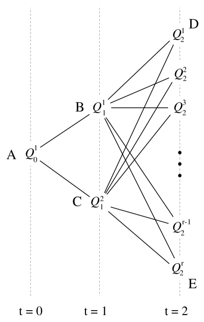
Figure 3: A double-slit experiment.

The source $A$ is represented by a single qubit labelled $\mathcal{Q}_{0}^{1}$ at time $t=0$ in the figure, which acts as a preparation switch. Given successful preparation, the labstate at time zero is given by $|\Psi,0)=\mathbb{A}_{1,0}^{+}|0,0)$. Subsequently, a signal could be detected at either of the two slits $B$, $C$. In the formalism, these are represented by qubits $\mathcal{Q}_{1}^{1}$and $\mathcal{Q}_{1}^{2}$ respectively, so the labstate is assumed to evolve according to the rule

$$|\Psi,0)\equiv\mathbb{A}_{1,0}^{+}|0,0)\rightarrow\mathbb{U}_{1,0}\mathbb{A}_{1,0}^{+}|0,0)=\left\{\alpha\mathbb{A}_{1,1}^{+}+\beta\mathbb{A}_{2,1}^{+}\right\}|0,1),$$ (61)

where $|\alpha|^{2}+|\beta|^{2}=1$ and the apparatus assumed isolated.

Now if either slit $B$ or $C$ were blocked off, the other slit would act as a preparation switch at time $1$ with $r_{2}$ possible one-signal outcomes subsequently at time $2$. Each one of these potential outcomes would be detected at an ESD $\mathcal{D}_{2}^{i}$ on the screen $DE$, and hence identified with a qubit $\mathcal{Q}_{2}^{i}$ in $H_{2}$, the Heisenberg net at time $2$. Here $i$ runs from $1$ to $r_{2}$, the number of distinct sites on the screen where a signal could be seen. Therefore we may write

$$\mathbb{A}_{i,1}^{+}|0,1)\rightarrow\mathbb{U}_{2,1}\mathbb{A}_{i,1}^{+}|0,1)=\sum_{j=1}^{r_{2}}\Psi^{j,i}\mathbb{A}_{j,2}^{+}|0,2),$$ (62)

where $i=1,2$ and $\Psi^{j,i}\equiv U_{2,1}^{2^{j-1},2^{i-1}}$. This assumes that one-signal states evolve into one-signal states only, an assumption which will undoubtedly depend on the physics of the situation. The double slit experiment in quantum optics is normally conducted in regimes where single-photon dynamics holds, so this is assumed here.

Semi-unitarity of evolution between times $1$ and $2$ imposes the rules

$$\sum_{j=1}^{r_{2}}[\Psi^{j,i}]^{\ast}\Psi^{j,k}=\delta_{ik},\ \ \ \ \ i,k=1,2.$$ (63)

With this information and assuming both slits open, we conclude that the labstate evolves from the initial labstate via the rule

$$|\Psi,0)\rightarrow\mathbb{U}_{2,1}\mathbb{U}_{1,0}|\Psi,0)=\sum_{j=1}^{r_{2}}\{\alpha\Psi^{j,1}+\beta\Psi^{j,2}\}\mathbb{A}_{j,2}^{+}|0,2).$$ (64)

We may immediately read off from this the final state amplitudes and hence determine the conditional probability of a signal being seen at any given site. We find

$$P\left(j,2|\Psi,0\right)=|\alpha|^{2}|\Psi^{j,1}|^{2}+|\beta|^{2}|\Psi^{j,2}|^{2}+\alpha^{\ast}\beta[\Psi^{j,1}]^{\ast}\Psi_{j,2}+\alpha\beta^{\ast}\Psi^{j,1}[\Psi^{j,2}]^{\ast},$$ (65)

for an outcome such that detector $j$ registers a signal and all the other remain void. The first two terms on the right hand side correspond to classical expectations whilst the remaining terms correspond to quantum interference terms. It is easy to prove that total probability is conserved, i.e., $\sum_{j=1}^{r_{2}}P(j,2|\Psi,0)=1.$

If the labstate arrived at the two slits such that the coefficients $\alpha$ and $\beta$ were randomly correlated in phase, then a classical ensemble averaging procedure would eliminate the interference terms in the above. Then we would have$\ P\left(j,2|\Psi,0\right)=|\alpha|^{2}|\Psi^{j,1}|^{2}+|\beta|^{2}|\Psi^{j,2}|^{2}$, which corresponds to classical probability expectations. In such a case, the experiment would look like one with two independent sources. From this sort of discussion, we conclude that it is the experimental context which is the source of wave-particle duality, and not the properties of an SUO alone.

24 Beam splitters

Quantum optics experiments are remarkable in consisting generally of modular components, such as beam-splitters, Wollaston prisms, mirrors, phase-shifters and other devices, connected by photonic pathways. In this section we discuss beam-splitters, which are mechanisms for superposing quantum amplitudes. In general such a module will form part of a greater network, as in the Mach-Zehnder interferometer discussed below, but in order to understand its structure better we shall first discuss the beam-splitter as if it were a complete piece of apparatus.

A typical beam-splitter $BS$ consists of two input ports labelled $a$ and $b$ in Figure $4$, and two output ports labelled $c$ and $d$. Considering a beam-splitter as a separate piece of apparatus in its own right, an experiment involving it would be described in QDN by a rank-$2$ net $\mathcal{Q}_{n}^{a}\otimes\mathcal{Q}_{n}^{b}$ evolving to a rank-$2$ net $\mathcal{Q}_{n+1}^{c}\otimes\mathcal{Q}_{n+1}^{d}$.

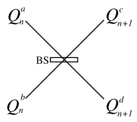
Figure 4: A beam-splitter.

At this point we simplify our notation further, in a form which has proved convenient for rapid calculations. Using the computation basis, signal states at time $n$ are written $i\equiv|i,n)$ whilst those at time $n+1$ are written $\bar{j}\equiv|j,n+1)$. We write $i\cdot j\equiv|i,n)(j,n|$, $\bar{\imath}\cdot j\equiv|i,n+1)(j,n|$, $A_{a}^{+}\equiv\mathbb{A}_{a,n}^{+}$, $\bar{A}_{c}^{+}\equiv\mathbb{A}_{c,n+1}^{+}$, $U\equiv\mathbb{U}_{n+1,n}$, and so on. In this notation, the signal operators at time $n$ are given by

$$A_{a}^{+}=1\cdot 0+3\cdot 2,\ \ \ A_{b}^{+}=2\cdot 0+3\cdot 1$$ (66)

and similarly for $\bar{A}_{c}^{+}$, $\bar{A}_{d}^{+}$.

Next, we specify the dynamics in terms of the computation basis vectors. The properties of a beam-splitter are encapsulated by the rules

$$\begin{array}[]{lll}0\rightarrow U0=\bar{0},&&1\rightarrow U1=\alpha\bar{1}+\beta\bar{2},\\ 2\rightarrow U2=\gamma\bar{1}+\delta\bar{2},&&3\rightarrow U3=\bar{3},\end{array}$$ (67)

where the complex coefficients $\alpha,\beta,\gamma,\delta$ satisfy the semi-unitary relations

$$|\alpha|^{2}+|\beta|^{2}=|\gamma|^{2}+|\delta|^{2}=1,\ \ \ \alpha^{\ast}\gamma+\beta^{\ast}\delta=0.$$ (68)

This assumes the beam-splitter is lossless. It is not necessary at this stage to assume the symmetrical case $|\alpha|^{2}\ =|\beta|^{2}=\tfrac{1}{2}$. In general, our formalism will be applied in the ideal, lossless and non-symmetric case.

The relations (67) have a wider applicability than just to beam-splitters. They can be used also to describe the Stern-Gerlach experiment, which involves electrons rather than photons. In that experiment, it is conventional to use only one incoming port, and then the experiment looks formally like a rank-$1$ net evolving into a rank-$2$ net. However, we could in principle reverse one of the out-beams back into the same inhomogeneous magnetic field and in that case, we would expect that the single reversed beam would split into two outgoing components, not one. One of these would be identifiable with the original in-port beam, whilst the existence of the other one would demonstrate that in fact the Stern-Gerlach experiment has essentially the same architecture as a beam-splitter.

Both beam-splitter and Stern-Gerlach devices represent specific realizations of a $2-2$ process, involving a rank-$2$ register evolving unitarily into another rank-$2$ register. The only significant difference between these realizations are the specific values of the coefficients $\alpha,\beta,\gamma$ and $\delta$, which are context-dependent, i.e., depend on the information held by the observer as to the physical interpretation of the signals being generated. The fact that the same structure of mathematics can be used for beam-splitters and Stern-Gerlach experiments reflects the fact that QDN can be regarded as a general formalism for the description of the logical architecture of any quantum experiment.

From the above, we use completeness to deduce

$$U=\bar{0}\cdot 0+\left\{\alpha\bar{1}+\beta\bar{2}\right\}\cdot 1+\left\{\gamma\bar{1}+\delta\bar{2}\right\}\cdot 2+\bar{3}\cdot 3.$$ (69)

Because there is no change of rank, this operator satisfies the unitarity rules $U^{+}U=I$, $UU^{+}=\bar{I}$, where $I$ and $\bar{I}$ are the identity operators for the registers $\mathcal{Q}_{n}^{a}\otimes\mathcal{Q}_{n}^{b}$ and $\mathcal{Q}_{n+1}^{c}\otimes\mathcal{Q}_{n+1}^{d}$ respectively. In order to prove the relationship $UU^{+}=\bar{I}$, we note that $U^{+}$ is in this case also a semi-unitary operator, and therefore the coefficients $\alpha,\beta,\gamma$ and $\delta$ satisfy the conjugate relations

$$|\alpha|^{2}+|\gamma|^{2}=|\beta|^{2}+|\delta|^{2}=1,\ \ \ \alpha^{\ast}\beta+\gamma^{\ast}\delta=0.$$ (70)

Hence we conclude $|\alpha|=|\delta|$ and $|\beta|=|\gamma|$. With this information it is easy to relate our matrices to those given by Zeilinger in his matrix formulation of the beam-splitter [32].

With all this information, we can work out the rules for the evolution of the signal operators. We find

$$A_{a}^{+} \rightarrow UA_{a}^{+}U^{+}=\left\{\alpha\bar{1}+\beta\bar{2}\right\}\cdot\bar{0}+\bar{3}\cdot\left\{\gamma^{\ast}\bar{1}+\delta^{\ast}\bar{2}\right\},$$

$$A_{b}^{+} \rightarrow UA_{b}^{+}U^{+}=\left\{\gamma\bar{1}+\delta\bar{2}\right\}\cdot\bar{0}+\bar{3}\cdot\left\{\alpha^{\ast}\bar{1}+\beta^{\ast}\bar{2}\right\}.$$ (71)

It can be verified that the signal algebra (18-19) is invariant to this transformation.

The rules for the evolution of the signal operators can be given in the more useful form

$$A_{a}^{+} \rightarrow UA_{a}^{+}U^{+}=\alpha\bar{A}_{c}^{+}+\beta\bar{A}_{d}^{+}+\bar{X}_{a},$$

$$A_{b}^{+} \rightarrow UA_{b}^{+}U^{+}=\gamma\bar{A}_{c}^{+}+\delta\bar{A}_{c}^{+}+\bar{X}_{b},$$ (72)

where

$$\bar{X}_{a}\equiv\bar{3}\cdot[(\gamma^{\ast}-\beta)\bar{1}+(\delta^{\ast}-\alpha)\bar{2}],\ \ \ \bar{X}_{b}\equiv\bar{3}\cdot\left[(\alpha^{\ast}-\gamma)\bar{1}+(\beta^{\ast}-\delta)\bar{2}\right]$$ (73)

are operators which annihilate the void state. The significance of this representation of the dynamics is that for single-signal processes, such as one-photon processes commonly studied in quantum optics, the $\bar{X}$ operators can be ignored. Therefore, in the general situation shown in Figure $4$, the dynamics of the in-ports associated with a beam-splitter can be written in the effective form

$$\mathbb{A}_{a,n}^{+} \rightarrow\mathbb{U}_{n+1,n}\mathbb{A}_{a,n}^{+}\mathbb{U}_{n+1,n}^{+}\sim\alpha\mathbb{A}_{c,n+1}^{+}+\beta\mathbb{A}_{d,n+1}^{+},$$

$$\mathbb{A}_{b,n}^{+} \rightarrow\mathbb{U}_{n+1,n}\mathbb{A}_{b,n}^{+}\mathbb{U}_{n+1,n}^{+}\sim\gamma\mathbb{A}_{c,n+1}^{+}+\delta\mathbb{A}_{d,n+1}^{+},$$ (74)

provided we restrict attention to one-photon processes. This justifies our usage of such approximations in our earlier work, which were derived using intuition [11].

25 The Mach-Zehnder interferometer

In the following, we shall drop explicit reference to time. The reasons for this are related to persistence and the relationship between photons and wave-trains, and are discussed further in later sections.

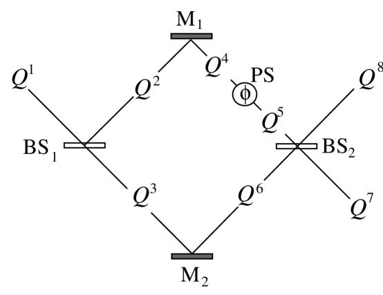
Figure 5: The Mach-Zehnder interferometer

The well-known Mach-Zehnder (MZ) interferometer, shown in Figure $5$, provides a useful testbed for the application of our formalism. A monochromatic beam of light is first passed through a beam-splitter $BS_{1}$. Each emergent component is then passed onto a separate mirror, denoted $M_{1}$ or $M_{2}$, which changes its phase by an amount $e^{i\mu_{1}}$ or $e^{i\mu_{2}}$ respectively. The component reflected from $M_{1}$ is then passed through a sample or device which changes its phase by an amount $e^{i\phi}$, and then both components are passed through another beam-splitter $BS_{2}$ onto two photon detectors. In Figure $5$ we show qubits which might be placed at various places to detect photon signals, if that were desired or planned by the experimentalist.

The strategy here is to invoke just as many qubits as needed to describe the essential logical structure of the device. If we wished to model the physics in a much more complete but inefficient and mostly redundant way, we might consider a much greater number of qubits, placed virtually everywhere along the optical paths that the light might take. This would then begin to look more like a quantum field theoretic description of the experiment. It is actually rare for quantum field theory to be applied in full detail to a quantum experiment performed over finite regions of time and space, and QDN is no different in this respect. Our experience with the formalism suggests that the qubits shown, labelled from $1$ to $8,$ represent a reasonable basis to describe the experiment.

In real experiments with such devices, the various parts of the apparatus persist during any given run, and we find it useful to encode that feature here. Hence we shall work with a rank-$8$ quantum register, with the various qubits labelled $1$ to $8$ as shown. Qubit $1$ acts as a preparation switch whilst qubits $7$ and $8$ act as outcome detectors.

Consider a pulse of light starting at the preparation switch $\mathcal{Q}^{1}$ at time $0$. The initial state is denoted by

$$|\Psi,0)=\mathbb{A}_{1,0}^{+}|0,0).$$ (75)

After passage through the first beam-splitter, $BS_{1}$, the discussion in the preceding section justifies us in writing

$$\mathbb{A}_{1,0}^{+}\rightarrow\mathbb{U}_{1,0}\mathbb{A}_{1,0}^{+}\mathbb{U}_{1,0}^{+}\sim\alpha_{1}\mathbb{A}_{2,1}^{+}+\beta_{1}\mathbb{A}_{3,1}^{+},$$ (76)

because single photon signal dynamics is assumed. Here $|\alpha_{1}|^{2}+|\beta_{1}|^{2}=1$ and only one in-port of $BS_{1}$ is being used. Reflection at the mirrors $M_{1}$, $M_{2}$ gives phase changes of the form

$$\mathbb{A}_{2,1}^{+}\rightarrow e^{i\mu_{1}}\mathbb{A}_{4,2}^{+},\ \ \ \mathbb{A}_{3,1}^{+}\rightarrow e^{i\mu_{2}}\mathbb{A}_{6,2}^{+}.$$ (77)

The phase-shift device $PS$ gives

$$\mathbb{A}_{4,2}^{+}\rightarrow e^{i\phi}\mathbb{A}_{5,2}^{+,}$$ (78)

where we assume there is essentially zero time delay. Finally, passage through the second beam-splitter $BS_{2}$ gives

$$\mathbb{A}_{5,2}^{+}\rightarrow\alpha_{2}\mathbb{A}_{8,3}^{+}+\beta_{2}\mathbb{A}_{7,3}^{+},\ \ \ \mathbb{A}_{6,2}^{+}\rightarrow\gamma_{2}\mathbb{A}_{8,3}^{+}+\delta_{2}\mathbb{A}_{7,3}^{+}.$$ (79)

Taking all changes together, we may write

$$|\Psi,0)=\mathbb{A}_{1,0}^{+}|0,0)\rightarrow \left[\alpha_{1}\alpha_{2}e^{i(\mu_{1}+\phi)}+\beta_{1}\gamma_{2}e^{i\mu_{2}}\right]\mathbb{A}_{8,3}^{+}|0,3)+$$

$$[\alpha_{1}\beta_{2}e^{i(\mu_{1}+\phi)}+\beta_{1}\delta_{2}e^{i\mu_{2}}]\mathbb{A}_{7,3}^{+}|0,3).$$ (80)

From this we may immediately read off the two detection amplitudes:

$$\mathcal{A}\left(8,3|\Psi,0\right) =\alpha_{1}\alpha_{2}e^{i(\mu_{1}+\phi)}+\beta_{1}\gamma_{2}e^{i\mu_{2}},$$

$$\mathcal{A}\left(7,3|\Psi,0\right) =\alpha_{1}\beta_{2}e^{i(\mu_{1}+\phi)}+\beta_{1}\delta_{2}e^{i\mu_{2}}.$$ (81)

Final state probabilities are then given by the rule

$$P\left(8|\Psi\right)=|\mathcal{A}\left(8,3|\Psi,0\right)|^{2},\ \ \ P\left(7|\Psi\right)=|\mathcal{A}\left(7,3|\Psi,0\right)|^{2},$$ (82)

and it may be verified that total probability is conserved. By tuning the various constants $\alpha_{1},\beta_{2},\ldots,\phi,$ the usual standard constructive and destructive quantum interference phenomena can be demonstrated readily, so we shall not discuss those effects further here, save for the following subsection.

25.1 The identity interferometer

As a check on the formalism, we consider the special case when the mirrors and the phase-shifter have no effect (i.e., $\mu_{1}=\mu_{2}=\phi=0)$ and the second beam-splitter, $BS_{1}$, effectively undoes the action of the first one, $BS_{2}$ This is achieved by setting

$$\alpha_{2}=\alpha_{1}^{\ast},\beta_{2}=\gamma_{1}^{\ast},\gamma_{2}=\beta_{1}^{\ast}\text{, }\delta_{2}=\delta_{1}^{\ast},$$ (83)

which is equivalent in SQM of representing the effect of $BS_{2}$ by the adjoint of the operator representing $BS_{1}.$ This gives

$$\mathcal{A}\left(8,3|\Psi,0\right)=|\alpha_{1}|^{2}+|\beta_{1}|^{2}=1,\ \ \ \mathcal{A}\left(7,3|\Psi,0\right)=\alpha_{1}\gamma_{1}^{\ast}+\beta_{1}\delta_{1}^{\ast}=0,$$ (84)

as expected.

26 Nested and serial networks

One of the advantages of the QDN formalism is that it allows an efficient approach to the calculation of amplitudes for extended networks, such as those consisting of two or more M-Z interferometers coupled together in series or parallel, with a consequent increase in the number of out-ports. We can imagine “plugging in” as many M-Z modules into networks of any desired topology as we wish, and the formalism should be able to handle them relatively straightforwardly. Currently, we are investigating the viability of encoding the formalism into a computer-algebra package, which should give an efficient method for calculating outcome probabilities for networks of great complexity.

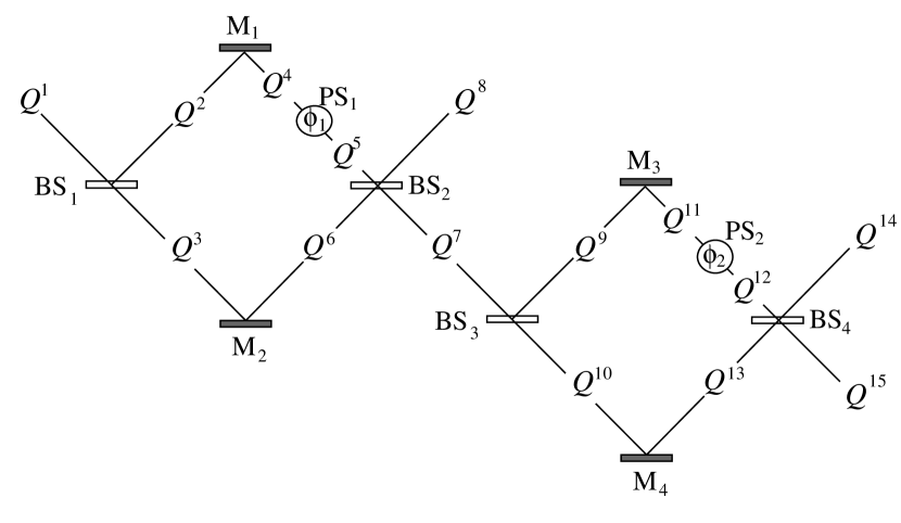
Figure 6: Nested Mach-Zehnder interferometers

As an example of a serial network, consider the network shown in Figure $6$, where one of the out-ports (number $7)$ of one M-Z interferometer is channelled into the in-port of a duplicate interferometer. The total number of detector sites is now increased to three, which are represented by qubits $8$, $14$ and $15.$

We may use the above calculation to determine the further evolution of output port $7$, which gives

$$\mathbb{A}_{7}^{+}\sim \left[\alpha_{3}\alpha_{4}e^{i(\mu_{3}+\phi_{2})}+\beta_{3}\gamma_{4}e^{i\mu_{4}}\right]\mathbb{A}_{14}^{+}+$$

$$[\alpha_{3}\beta_{4}e^{i(\mu_{2}+\phi_{2})}+\beta_{3}\delta_{4}e^{i\mu_{4}}]\mathbb{A}_{15}^{+},$$ (85)

where we do not show the dependence on time. Inserting this into (80) gives

$$|\Psi)=\mathbb{A}_{1}^{+}|0)\rightarrow \left[\alpha_{1}\alpha_{2}e^{i(\mu_{1}+\phi)}+\beta_{1}\gamma_{2}e^{i\mu_{2}}\right]\mathbb{A}_{8}^{+}|0)+$$

$$[\alpha_{1}\beta_{2}e^{i(\mu_{1}+\phi)}+\beta_{1}\delta_{2}e^{i\mu_{2}}]\left[\alpha_{3}\alpha_{4}e^{i(\mu_{3}+\phi_{2})}+\beta_{3}\gamma_{4}e^{i\mu_{4}}\right]\mathbb{A}_{14}^{+}|0)+$$

$$[\alpha_{1}\beta_{2}e^{i(\mu_{1}+\phi)}+\beta_{1}\delta_{2}e^{i\mu_{2}}][\alpha_{3}\beta_{4}e^{i(\mu_{2}+\phi_{2})}+\beta_{3}\delta_{4}e^{i\mu_{4}}]\mathbb{A}_{15}^{+}|0),$$ (86)

from which the outcome probability amplitudes can be read off immediately.

The potential complexity of such networks does not mean more than one photon would be detected in any given run. That depends on the dynamics of individual modules. If for example, one of the above output ports was fed into a module that produced a two-signal outcome, corresponding to a two-photon state, then we would find a final state with two-signal components. This is easily encoded into our formalism.

The potential value of QDN is that an increase in the complexity of a network can be handled relatively easily. In SQM, an increase in the number of out-ports requires special attention. It was this sort of issue that led to the development of the POVM formalism, because in the more conventional PVM approach, the dimensions of the Hilbert space involved is considered fixed [21]. Once an arbitrary number of output channels is involved, the simple PVM strategy fails.

We shall illustrate in the next section the difference between the POVM approach and our approach by analyzing a network studied by Brandt using the conventional POVM formalism. In fact, it is known that the POVM formalism can be turned into a PVM formalism by embedding everything into a sufficiently big Hilbert space. This may involve the introduction of an auxiliary space known as an ancilla. Generally, we do not find that approach so convincing, as it is not obvious to us how the auxiliary spaces relate to the apparatus.

It is at this point that a criticism of QDN could be made: it looks like another way of embedding the conventional formalism into a sufficiently big Hilbert space so as to allow the operation of a PVM formalism. Neumark’s theorem says that this is always possible. However, that would be to miss the point. The QDN strategy is based on the physics of observation and not by any desire to have a PVM formalism per se, although that is always desirable. A qubit is not introduced into our approach unless there is a physical reason for it and every aspect of the formalism is justifiable in terms of the experimental procedures carried out by the observer. The orthonormality of the signal basis comes from the classical nature of observation as it is done in real experiments.

A more serious criticism of our formalism, already mentioned, is that it leads to very large Hilbert spaces. In the example shown in Figure $6$, the fifteen qubits form a quantum register of dimension $2^{15}=32768$, which seems excessive considering there are just three out-ports. However, the dimensions of the quantum registers we employ seem excessive simply because persistence is assumed and there is so much more we can do with the formalism. At each point where we place a qubit, we can insert additional modules such as beam-splitters and so on, leading to new experimental architecture. There is no reason to restrict this to diagrams which are planar, either. We can consider time-dependent apparatus (which we did not do in our discussion of the M-Z interferometer above), and we can consider situations where several runs coexist at the same time. What this means is that parts of a network may be showing signals which would conventionally be identified with one in-state, whilst other parts would behave is if they were carrying signals from an earlier or later run. Something like this happens in high-energy particle physics experiments, when separate pulses of charged particles are kept circulating in a collider ring all at the same time until they are diverted and smashed into a target at separate times.

In the sort of calculations we have encountered, the relatively high dimensionality of the quantum registers involved have not been a problem, because as we have shown, the calculations can be handled usually in terms of the signal operators $\mathbb{A}_{i}^{+}$, which leads to a great deal of economy.

Another point in defence of QDN is that its objective of modelling apparatus rather than SUOs would create difficult problems for SQM. In particular, quantum field theory requires relatively sophisticated mathematical machinery, and any attempt to model apparatus in terms analogous to those of QDN would require heavy computation. Schwinger’s source theory approach is perhaps the closest quantum field theoretic analogue to QDN [30]. There are also parallels between S-matrix theory and QDN, particularly in the way on-shell amplitudes are iterated [33].

27 Time dependence and Bohmian mechanics

In the above calculation, the time dependence was dropped for notational convenience. The reason why this is permissible in a number of quantum optics scenarios is that “monochromatic” photons are associated with wave-trains of approximately fixed wavelength $\lambda$, and the physical length of such a wave-train can be very long compared to $\lambda$ itself. When such a long wave-train passes through an apparatus, the result is that over an extended period of time, it looks as if the electromagnetic field is persistent throughout the apparatus, and so time-dependence can be ignored.

If a relatively short wave-train is passed through a Mach-Zehnder network, however, it is possible that no interference would take place, because waves components travelling along different optical paths would arrive at the second beam-splitter at different times and so miss each other. In such a scenario, our approach would have to take the time dependence of the labstate more carefully into account, most probably by introducing additional qubits to incorporate the additional optical path lengths, but this would not be an issue which the formalism could not handle straightforwardly. Give it enough qubits and QDN can model the universe [9].

Wave-trains do not “contain” photons as such. Paul [10] gives examples of experiments where the average number of photons per wave-train is less than one. Such wave-trains are properly regarded as probability amplitudes, not structural components of SUOs in the way Schrödinger believed.

Bohmian mechanics [20] is the outcome of the type of thinking that motivated first de Broglie and then Schrödinger towards the development of wave-mechanics. It retains the interest of a proportion of theorists who adhere to the conditioning of the classical world view, and can be thought of as the opposite side of the spectrum of quantum theories to QDN. Rather than abandon SUOs, Bohmian mechanics turns the wave-function itself into a type of SUO, with an assumed classical existence in one form or another. Such theories have little or no regard for the issues involved with information extraction, and are regarded by us as severely flawed in that respect.

An issue in Bohmian mechanics, where it is imagined that particles are guided by “pilot waves”, is the existence of “empty” waves containing no particle. In the double slit experiment, for example, Bohmian theorists would have to accept that according to their principles, a particle was guided to go through one slit and not the other, which means that an empty wave has passed through one of the slits. It is not clear in that approach what happens to these empty waves once the particle has landed on a screen. Presumably, there has to be some mechanism in Bohmian mechanics for signals to be sent from the impact site to kill off any empty waves still propagating elsewhere in the universe. No such requirement occurs in QDN.

28 A POVM network calculation

We turn now to a variant of the Mach-Zehnder interferometer studied by Brandt using the POVM formalism in SQM [34, 35]. The network is shown in Figure $7$.

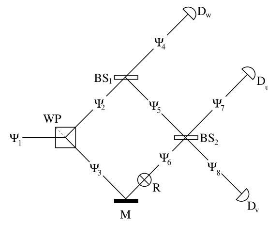
Figure 7: Brandt’s POVM network.

In standard terminology, a beam $\Psi_{1}$ passes through a Wollaston prism $WP$, and its output channels $\Psi_{2}$, $\Psi_{3}$ are passed to a beam-splitter $BS_{1}$ and mirror $M$ respectively. Beam-splitter $BS_{1}$ has transmission and reflection coefficients characterized by an angle $\theta$ in a specific way. Its transmitted wave $\Psi_{4}$ is detected at detector $D_{w}$ whilst the reflected wave $\Psi_{5}$ is passed into beam-splitter $BS_{2}.$ After wave $\Psi_{3}$ has reflected off mirror $M$, its polarization is rotated by $90^{\circ}$ at $R$ and then it is passed on to beam-splitter $BS_{2}$ in order to interfere with $\Psi_{5}.$ Detectors $D_{u}$ and $D_{v}$ act as out-ports for beam-splitter $BS_{2}.$

In his discussion, Brandt takes the initial state $|\Psi_{1}\rangle$ to be a linear combination of non-orthogonal normalized states $|u\rangle$, $|v\rangle$ such that $|\Psi_{1}\rangle=\alpha|u\rangle+\beta|v\rangle$, with $\langle u|v\rangle=\cos\theta\neq-1$ and

$$|\alpha|^{2}+|\beta|^{2}+(\alpha^{\ast}\beta+\alpha\beta^{\ast})\cos\theta=1.$$ (87)

The outcomes are discussed in terms of POVM operators $E_{u\text{ }},E_{v}$ and $E_{w}$, which satisfy the relations

$$E_{u}=\frac{I_{\mathcal{H}}-|v\rangle\langle v|}{1+\cos\theta},\ E_{v}=\frac{I_{\mathcal{H}}-|u\rangle\langle u|}{1+\cos\theta},\ \ \ E_{w}=I_{\mathcal{H}}-E_{u}-E_{v}.$$ (88)

Here $I_{\mathcal{H}}\equiv E_{u}+E_{v}+E_{w}$ is the identity operator for the two-dimensional Hilbert space with non-orthogonal normalized basis $\{|u\rangle,|v\rangle\}$. The three outcome probabilities are given by

$$\begin{array}[]{ccccc}P\left(u|\Psi_{1}\right)&=&\langle\Psi_{1}|E_{u}|\Psi_{1}\rangle&=&|\alpha|^{2}(1-\cos\theta),\\ P\left(v|\Psi_{1}\right)&=&\langle\Psi_{1}|E_{v}|\Psi_{1}\rangle&=&|\beta|^{2}(1-\cos\theta),\\ P\left(w|\Psi_{1}\right)&=&\langle\Psi_{1}|E_{w}|\Psi_{1}\rangle&=&|\alpha+\beta|^{2}\cos\theta,\end{array}$$ (89)

which add up to unity.

The quantum register discussion assigns qubits as shown in Figure $8$, so we need at least a rank-$8$ register.

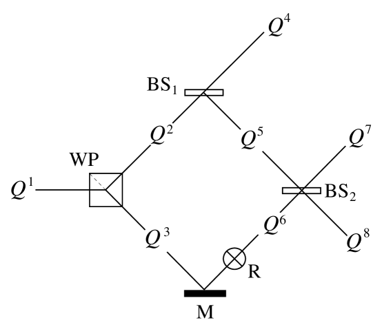
Figure 8: Qubit assignment for Brandt’s network.

The QDN calculation is based on Brandt’s parametrization of the various modules and goes as follows.

$i)$ The rules for a Wollaston prism are virtually the same as for a beam-splitter, except for having a different physical interpretation. The two output ports, for example, carry different photon polarizations. Wollaston prism $WP$ gives

$$\mathbb{A}_{1}^{+}\rightarrow\left(\alpha+\beta\right)\cos(\frac{{}_{1}}{{}^{2}}\theta)\mathbb{A}_{2}^{+}+\left(\alpha-\beta\right)\sin(\frac{{}_{1}}{{}^{2}}\theta)\mathbb{A}_{3}^{+},$$ (90)

where the angle $\theta$ is related to $\alpha$ and $\beta$ by relation (87);

$ii)$ the beam-splitter $BS_{1}$ gives

$$\mathbb{A}_{2}^{+}\rightarrow\sqrt{1-\tan^{2}(\frac{{}_{1}}{{}^{2}}\theta)}\mathbb{A}_{4}^{+}+i\tan(\frac{{}_{1}}{{}^{2}}\theta)\mathbb{A}_{5}^{+}.$$ (91)

Here the beam-splitter is finely tuned to the effects of the Wollaston prism $WP$ in a particular way, it being assumed that this is possible in a real experiment;

$iii)$ the mirror $M$ and the $90^{\circ}$ polarization rotation $R$ give

$$\mathbb{A}_{3}^{+}\rightarrow-\mathbb{A}_{6}^{+};$$ (92)

$iv)$ the beam splitter $BS_{2}$ gives

$$\mathbb{A}_{5}^{+}\rightarrow\frac{i}{\sqrt{2}}\mathbb{A}_{7}^{+}+\frac{1}{\sqrt{2}}\mathbb{A}_{8}^{+},\ \ \ \mathbb{A}_{6}^{+}\rightarrow\frac{1}{\sqrt{2}}\mathbb{A}_{7}^{+}+\frac{i}{\sqrt{2}}\mathbb{A}_{8}^{+}.$$ (93)

Here, beam-splitter $BS_{2}$ is assumed symmetric.

The net result is the evolution rule

$$\mathbb{A}_{1}^{+}\rightarrow\left(\alpha+\beta\right)\sqrt{\cos\theta}\mathbb{A}_{4}^{+}-\alpha\sqrt{1-\cos\theta}\mathbb{A}_{7}^{+}+i\beta\sqrt{1-\cos\theta}\mathbb{A}_{8}^{+},$$ (94)

or

$$|\Psi_{out})=\left(\alpha+\beta\right)\sqrt{\cos\theta}|2^{3})-\alpha\sqrt{1-\cos\theta}|2^{6})+i\beta\sqrt{1-\cos\theta}|2^{7}).$$

From this we readily work out the conditional probabilities

$$\begin{array}[]{ccccc}P\left(w|\Psi_{0}\right)&\equiv&|(2^{3}|\Psi_{out})|^{2}&=&|\alpha+\beta|^{2}\cos\theta,\\ P\left(u|\Psi_{0}\right)&\equiv&|(2^{6}|\Psi_{out})|^{2}&=&|\alpha|^{2}\left(1-\cos\theta\right),\\ P\left(v|\Psi_{0}\right)&\equiv&|(2^{7}|\Psi_{out})|^{2}&=&|\beta|^{2}\left(1-\cos\theta\right),\end{array}$$ (95)

in complete agreement with Brandt’s calculation.

A few comments about the respective merits of the two approaches are in order here. First, the POVM approach attempts to keep the discussion to within the Hilbert space of the original state, i.e., in two dimensions in this particular example. The need to accommodate three possible outcomes then forces a break with the strict PVM formalism of von Neumann [21], which would require all outcome states to be orthogonal. The quantum register calculation works naturally within a PVM setting because of the physics of observation. QDN was not motivated by any desire to use the Neumark theorem, which says that a POVM description can always be replaced by an equivalent PVM setting by introducing extra Hilbert space dimensions.

Another issue is the physical significance of the non-orthogonality of the vectors $|u\rangle$ and $|v\rangle$ in the POVM discussed here. Our approach avoids non-orthogonality because we adhere to the principle that the dual register basis consists of elements representing classically meaningful questions, and these are mutually exclusive. It is not clear to us what the physical significance of the non-zero inner product $\langle u|v\rangle=\cos\theta$ is, other than as formal device, within an SQM setting, designed to reflect the physical properties of the preparation apparatus, not those of the detectors $D_{u}$ and $D_{v}$.

A final point about POVMs is that they are usually applied in situations involving mixed states, and the density matrix formulation becomes necessary. The QDN formalism should be able to deal with such situations readily. A particularly interesting possibility arises here: the idea that the apparatus itself could become mixed (i.e., uncertain). In such a scenario, the observer might have to assign a probability distribution to more than one Heisenberg net at a given time, and these nets could have different ranks. Such a scenario would require an enhanced version of density matrix theory, perhaps representing a step in the development of a more comprehensive theory of the physics of observation than is currently available. This is one of the lines of further enquiry which we hope to report on presently.

29 Higher signal-rank experiments

The examples studied above correspond to signal-rank one dynamics, such as one-photon experiments in quantum optics, but these are a subset of all possible experiments. We can just as easily discuss scenarios involving two or more photons, and these raise the possibility of entanglement, in addition to the superposition involved in the one-photon case.

29.1 Independent experiments

In the real world, different laboratories conduct quantum optics experiments independently of each other, and any comprehensive theory should be able to describe that scenario naturally, and allow for the possibility of dynamical interaction between laboratories. QDN describes such scenarios naturally by tensoring separate quantum registers together into larger super-registers. A super-labstate in such a super-register representing independent laboratories would remain factorizable as long as there was no information exchange between those laboratories in any form. Each factor would be associated with a separate laboratory conducting its own experiment. Separability would endure until such a time as there was an interaction between laboratories, at which point the super-labstate would become entangled.

To illustrate the point, consider two independent Stern-Gerlach experiments carried out simultaneously, according to some superobserver in contact with each independent laboratory. Figure $9$ show the basic set-up. Experiment $1$ has a preparation switch $\mathcal{Q}^{1}$ and output qubits $\mathcal{Q}^{2},\mathcal{Q}^{3}$ whilst Experiment $2$ has preparation switch $\mathcal{Q}^{4}$ and output qubits $\mathcal{Q}^{5}$ and $\mathcal{Q}^{6}$.

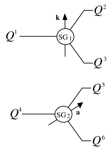
Figure 9: Super-network containing two subnetworks.

The super-observer describes the two experiments in terms of the rank-$6$ quantum register $\mathcal{R}^{6}\equiv\mathcal{Q}^{1}\otimes\mathcal{Q}^{2}\otimes\mathcal{Q}^{3}\otimes\mathcal{Q}^{4}\otimes\mathcal{Q}^{5}\otimes\mathcal{Q}^{6}$. Assuming each laboratory starts a run at the same time, then the initial labstate is given by

$$|\Psi_{in})=\mathbb{A}_{1}^{+}\mathbb{A}_{4}^{+}|0)=|100100)=|2^{0}+2^{3})=|9)=|100)_{123}\otimes|100)_{456},$$ (96)

where the last expression on the right-hand side shows the separability of the labstate. This means that according to the super-observer, their labstate is a two-signal state, but each independent laboratory would think it was dealing with a one-signal state.

If each experiment is truly independent and carries out a run simultaneously with the other laboratory according to the time of the super-observer, then evolution is given by

$$\mathbb{A}_{1}^{+} \rightarrow\alpha\mathbb{A}_{2}^{+}+\beta\mathbb{A}_{3}^{+},\;\;\;\;\;|\alpha|^{2}+|\beta|^{2}=1,$$

$$\mathbb{A}_{4}^{+} \rightarrow\gamma\mathbb{A}_{5}^{+}+\delta\mathbb{A}_{6}^{+},\;\;\;\;\;|\gamma|^{2}+|\delta|^{2}=1,$$ (97)

where independence of the laboratories means that there is no constraint relating the coefficients $\{\alpha,\beta\}$ with the coefficient $\left\{\gamma,\delta\right\}.$ The initial super-labstate then remains factorizable, i.e.,

$$|\Psi_{in})\rightarrow|\Psi_{out})=\left(\alpha\mathbb{A}_{2}^{+}+\beta\mathbb{A}_{3}^{+}\right)\left(\gamma\mathbb{A}_{5}^{+}+\delta\mathbb{A}_{6}^{+}\right)|0)=|\psi)_{123}\otimes|\phi)_{456},$$ (98)

where

$$|\psi)_{123} \equiv\alpha|0)_{1}|1)_{2}|0)_{3}+\beta|0)_{1}|0)_{2}|1)_{3},$$

$$|\phi)_{456} \equiv\gamma|0)_{4}|1)_{5}|0)_{6}+\delta|0)_{4}|0)_{5}|1)_{6}.$$ (99)

29.2 Change of signal number experiments

An interesting class of experiments involves changes of signal number induced by entanglement, an important example being given by experiments based on the EPR thought experiment [36]. It is most convenient to discuss such an experiment in terms of electron spin or photon polarization. We shall discuss it in terms of electron spin.

In the conventional terminology of SQM, such an experiment starts with the preparation of an entangled state of an electron-positron pair, with total spin zero. Subsequently, two observers, Alice and Bob measure spin components using separate Stern-Gerlach machines. Alice filters only electrons into her machine and observes their spin relative to the main field of her apparatus, which is aligned along the $\mathbf{k}-$axis. The other observer, Bob, filters only positrons into his machine, which has its main magnetic field aligned along some other direction, $\mathbf{a}$.

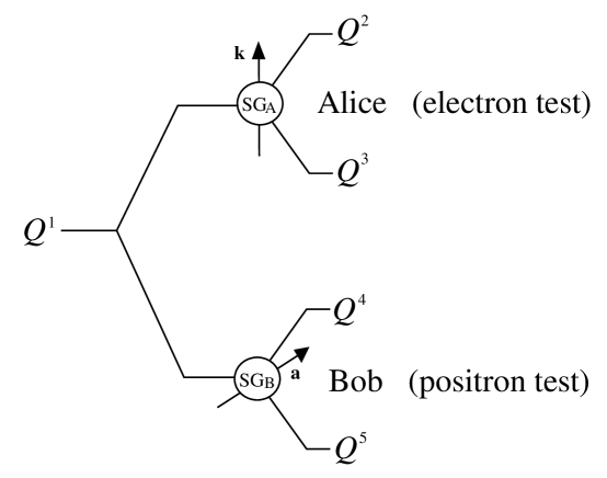
Figure 10: Change of signal rank experiment.

Assuming the initial state has total spin zero, the SQM representation of the initial state is given by

$$|\Psi\rangle=\frac{1}{\sqrt{2}}\left\{\begin{array}[]{c}\sin(\frac{{}_{1}}{{}^{2}}\theta)e^{-i\phi}|+\mathbf{k\rangle}_{-}\otimes|+\mathbf{a\rangle}_{+}+\cos(\frac{{}_{1}}{{}^{2}}\theta)e^{-i\phi}|+\mathbf{k\rangle}_{-}\otimes|-\mathbf{a\rangle}_{+}\\ -\cos(\frac{{}_{1}}{{}^{2}}\theta)|-\mathbf{k\rangle}_{-}\otimes|+\mathbf{a\rangle}_{+}+\sin(\frac{{}_{1}}{{}^{2}}\theta)|-\mathbf{k\rangle}_{-}\otimes|-\mathbf{a\rangle}_{+}\end{array}\right\},$$ (100)

where the subscript $(-)$ refers to the electron whilst $(+)$ refers to the positron.

The QDN interpretation is inherently different to the SQM interpretation. The initial labstate can be described as an entangled state of an electron and a positron only if the apparatus after state preparation permits such information to be extracted. According to our principles, positronium is considered an unstable elementary particle if it is observed as such, whereas if the apparatus can register electrons and positrons separately, then positronium can be described as an entangled state of an electron and a positron. This illustrates the point that entanglement is not an inherent property of an SUO, but depends on the context of observation.

Figure $10$ shows the QDN qubit assignment for this experiment. In the QDN description of the experiment, the preparation switch $\mathcal{Q}^{1}$ prepares an initial one-signal labstate $|\Psi,0)\equiv\mathbb{A}_{1,0}^{+}|0,0)$. The subsequent dynamics is given by

$$\mathbb{A}_{1,0}^{+}\rightarrow\mathbb{U}_{1,0}\mathbb{A}_{1,0}^{+}\mathbb{U}_{1,0}^{+} \sim\frac{\sin(\frac{{}_{1}}{{}^{2}}\theta)e^{-i\phi}}{\sqrt{2}}\mathbb{A}_{2,1}^{+}\mathbb{A}_{4,1}^{+}+\frac{\cos(\frac{{}_{1}}{{}^{2}}\theta)e^{-i\phi}}{\sqrt{2}}\mathbb{A}_{2,1}^{+}\mathbb{A}_{5,1}^{+}$$

$$-\frac{\cos(\frac{{}_{1}}{{}^{2}}\theta)}{\sqrt{2}}\mathbb{A}_{3,1}^{+}\mathbb{A}_{4,1}^{+}+\frac{\sin(\frac{{}_{1}}{{}^{2}}\theta)}{\sqrt{2}}\mathbb{A}_{3,1}^{+}\mathbb{A}_{5,1}^{+},$$ (101)

which means that the initial one-signal labstate evolves into an entangled two-signal labstate.

29.3 Two-particle interferometry

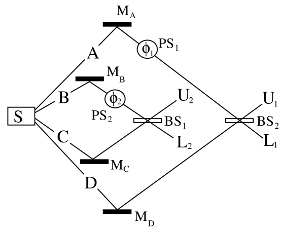
Figure 11: Experiment involving a two-photon source.

In $1989$, Horne, Shimony and Zeilinger discussed an experiment involving two-photon interferometry [37]. Their experimental is shown in Figure $11$. A source $S$ prepares an entangled two-photon state. A set of mirrors, $M_{A}$, $M_{B}$, $M_{C}$ and $M_{D}$ reflect various components of the prepared state through phase-changers $PS_{1}$ and $PS_{2}$ and onto beam-splitters $BS_{1}$ and $BS_{2}$. Finally, photon coincidence detectors $U_{1}$, $U_{2}$, $L_{1}$ and $L_{2}$ are placed as shown.

The initial state is described in terms of photon polarization vectors, and is given in the form [37]

$$|\Psi_{in}\rangle=\frac{1}{\sqrt{2}}\left\{|\mathbf{k}_{A}\rangle_{1}|\mathbf{k}_{C}\rangle_{2}+|\mathbf{k}_{D}\rangle_{1}|\mathbf{k}_{B}\rangle_{2}\right\}.$$ (102)

A standard calculation then gives the coincidence probabilities

$$\begin{array}[]{ccc}P(U_{1},U_{2}|\phi_{1},\phi_{2})=P\left(L_{1},L_{2}|\phi_{1},\phi_{2}\right)&=&\frac{1}{4}\left\{1+\cos(\phi_{2}-\phi_{1}+\theta)\right\},\\ P(U_{1},L_{2}|\phi_{1},\phi_{2})=P\left(L_{1},U_{2}|\phi_{1},\phi_{2}\right)&=&\frac{1}{4}\left\{1-\cos(\phi_{2}-\phi_{1}+\theta)\right\},\end{array}$$ (103)

where depends on the detailed relative placement of the mirrors, etc.

The QDN assignment of qubits is shown in Figure $12$. The preparation switch prepares a labstate which evolves to the equivalent of an entangled two-photon state, given by

$$\mathbb{A}_{1}^{+}\rightarrow\frac{1}{\sqrt{2}}\left\{\mathbb{A}_{2}^{+}\mathbb{A}_{4}^{+}+e^{i\theta}\mathbb{A}_{3}^{+}\mathbb{A}_{5}^{+}\right\}.$$ (104)

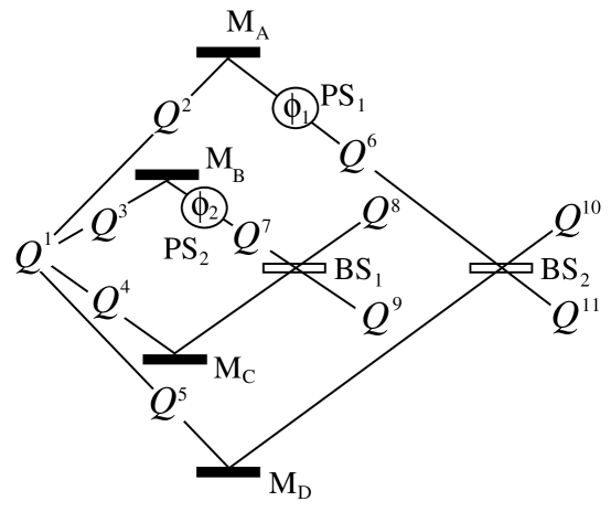
Figure 12: Qubit assignment for the experiment shown in Figure $11$.

Here the angle $\theta$ depends on the detailed placement of the various pieces of equipment. Ignoring the phase changes at the mirrors, which are the same and hence do not alter relative outcome probabilities, the various modules have the following effects:

$i)$ The phase changers $PS_{1}$, $PS_{2}$ give

$$\mathbb{A}_{2}^{+}\rightarrow e^{i\phi_{1}}\mathbb{A}_{6}^{+},\;\;\;\mathbb{A}_{3}^{+}\rightarrow e^{i\phi_{2}}\mathbb{A}_{7}^{+};$$ (105)

$ii)$ the beam splitters $BS_{1}$, $BS_{2}$ are symmetric and give

$$\mathbb{A}_{7}^{+} \rightarrow\frac{1}{\sqrt{2}}\left\{\mathbb{A}_{9}^{+}+i\mathbb{A}_{8}^{+}\right\},\;\;\;\mathbb{A}_{4}^{+}\rightarrow\frac{1}{\sqrt{2}}\left\{\mathbb{A}_{8}^{+}+i\mathbb{A}_{9}^{+}\right\},$$

$$\mathbb{A}_{4}^{+} \rightarrow\frac{1}{\sqrt{2}}\left\{\mathbb{A}_{10}^{+}+i\mathbb{A}_{11}^{+}\right\},\;\;\;\mathbb{A}_{6}^{+}\rightarrow\frac{1}{\sqrt{2}}\left\{\mathbb{A}_{11}^{+}+i\mathbb{A}_{10}^{+}\right\}.$$ (106)

Hence we arrive at the evolution rule

$$\mathbb{A}_{1}^{+} \rightarrow\frac{1}{2\sqrt{2}}\left\{e^{i\phi_{1}}-e^{i(\theta+\phi_{2})}\right\}\mathbb{A}_{8}^{+}\mathbb{A}_{11}^{+}+\frac{1}{2\sqrt{2}}\left\{ie^{i\phi_{1}}+ie^{i(\theta+\phi_{2})}\right\}\mathbb{A}_{8}^{+}\mathbb{A}_{10}^{+}$$

$$+\frac{1}{2\sqrt{2}}\left\{ie^{i\phi_{1}}+ie^{i(\theta+\phi_{2})}\right\}\mathbb{A}_{9}^{+}\mathbb{A}_{11}^{+}+\frac{1}{2\sqrt{2}}\left\{-e^{i\phi_{1}}+e^{i(\theta+\phi_{2})}\right\}\mathbb{A}_{9}^{+}\mathbb{A}_{10}^{+}.$$ (107)

From this, we can immediately read off the various coincidence amplitudes, and work out the coincidence probabilities, which are found to be

$$\begin{array}[]{lcc}P\left(8\ \&\ 10|\Psi_{in}\right)=P\left(9\ \&11|\Psi_{in}\right)&=&\frac{1}{4}\left\{1+\cos\left(\phi_{2}-\phi_{1}+\theta\right)\right\},\\ P\left(8\ \&\ 11|\Psi_{in}\right)=P\left(9\ \&\ 10|\Psi_{in}\right)&=&\frac{1}{4}\left\{1-\cos\left(\phi_{2}-\phi_{1}+\theta\right)\right\},\end{array}$$ (108)

in agreement with the standard calculation.

We note that after passage through the mirrors, the labstate behaves as if it were a super-labstate being analyzed by two separate laboratories, with separate apparatus $BS_{1}$ and $BS_{2}$. The entanglement of the super-labstate entanglement is then “undone” by the separate observations involved with these beam-splitters, and these never show entanglement per se in any individual outcome.

30 Particle decays

In this section we give a brief account of the QDN approach to particle decays [38]. The approach extends naturally to describe the quantum Zeno effect, the ammonium molecule and neutral Kaon decays.

We shall consider the quantum physics of what in SQM would be called an unstable particle, the initial state $X$ of which can decay into some multiparticle state $Y$. At all times total probability will be manifestly conserved. The momenta of the particles will be ignored here, the discussion being designed to illuminate the basic principles of the formalism only.

Typically, the sort of experiment of interest here can be repeated many times, and the formalism gives the quantum description of an ensemble of runs of a basic experiment. Clocks can always be reset, so a typical run of the experiment may be taken to start at time $t=0$, at which time the observer believes that they have prepared an $X$ state (to use the language of SQM). In QDN, this is represented by the labstate $|\Psi,0)\equiv\mathbb{A}_{X,0}^{+}|0,0)$, which is automatically normalized to unity.

By time $1$, the labstate will have changed from $|\Psi,0)$ to some new labstate $|\Psi,1)$ given by

$$|\Psi,1)=\alpha\mathbb{A}_{X,1}^{+}|0,1)+\beta\mathbb{A}_{Y_{1},1}^{+}|0,1),$$ (109)

where the complex numbers $\alpha$ and $\beta$ satisfy the semi-unitarity rule $|\alpha|^{2}+|\beta|^{2}=1$. The outcome possibilities of finding the void state $|0,1)$ or the two-signal state $\mathbb{A}_{X,1}^{+}\mathbb{A}_{Y_{1},1}^{+}|0,1)$ are excluded on dynamical grounds: any run with either of these outcomes would be discounted by the observer as contaminated by external influences (as happens in real experiments). From (109), the amplitude $\mathcal{A}(X,1|X,0)$ for the particle not to have decayed by time $1$ is given by

$$\mathcal{A}(X,1|X,0)\equiv(0,1|\mathbb{A}_{X,1}|\Psi,1)=\alpha$$ (110)

whilst the amplitude $\mathcal{A}(Y,1|X,0)$ for the particle to have made the transition to state $Y$ by time $1$ is given by

$$\mathcal{A}(Y,1|X,0)\equiv(0,1|\mathbb{A}_{Y_{1},1}|\Psi,1)=\beta.$$ (111)

Total probability is therefore conserved. Note that on the right hand side of (111), the label $Y$ is itself labeled by a subscript, in this case the number $1$, which is the time at which the amplitude is calculated for. The time at which a transition occurs is a crucial feature of the analysis, being directly related to the measurement issues discussed by Misra and Sudarshan [28].

The above process conserves signal class, so the dynamics can be discussed wholly in terms of the evolution of the signal operators rather than the labstates. For instance, evolution from time $0$ to $1$ can be given in the form

$$\mathbb{A}_{X,0}^{+}\rightarrow\mathbb{U}_{1,0}\mathbb{A}_{X,0}^{+}\mathbb{U}_{1,0}^{+}=\alpha\mathbb{A}_{X,1}^{+}+\beta\mathbb{A}_{Y_{1},1}^{+},$$ (112)

where $\mathbb{U}_{1,0}$ is a semi-unitary operator satisfying the rule $\mathbb{U}_{1,0}^{+}\mathbb{U}_{1,0}=\mathbb{I}_{0}$, with $\mathbb{I}_{0}$ being the identity for the initial register $\mathcal{R}_{0}\equiv\mathcal{Q}_{0}^{X}$. The above process involves a change in rank, since $\mathcal{R}_{1}\equiv\mathcal{Q}_{1}^{X}\mathcal{Q}_{1}^{Y_{1}}$. Because $r_{1}\equiv\dim\mathcal{R}_{1}>r_{0}\equiv\dim\mathcal{R}_{0}$, semi-unitarity of the evolution operator means that $\mathbb{U}_{1,0}\mathbb{U}_{1,0}^{+}\neq\mathbb{I}_{1}$, which is equivalent to irreversibility in SQM.

The description of the next stage of the process, from time $1$ to time $2$, is more subtle and involves the concept of null test [7]. In SQM, a null test is defined as any quantum test which extracts no information from an initial state. Physically, this corresponds to passing an outcome of a given apparatus through the same or equivalent apparatus, the net effect being that the state remains unchanged. For example, an electron emerging from a Stern-Gerlach apparatus $S_{0}$ in the spin-up state would pass through another Stern-Gerlach apparatus $S_{1}$ unscathed and still in its spin-up state, provided the magnetization axis of $S_{1}$ was in the same direction as that of $S_{0}$. In SQM, a null test is modelled mathematically by the fact that an eigenstate of an operator is also an eigenstate of the square of that operator.

In QDN, it is not the case that a null test involves no change whatsoever in the observer’s information of what is going on. The observer does have the information that time has passed during the null test, and that fact is registered in the observer’s memory. Moreover, in QDN, a labstate always changes in time, because the quantum register it is in changes with time. What is relevant is the set of components of a labstate, relative to the signal state basis at any given time. It is those components which are related to outcome probabilities. If those components do not change, then the observer may speak about the labstate as being constant in time, but the observer will also have an awareness that the state is evolving in time as well. In other words, the passage of time involves the observer as much as it involves the labstate.

Considering the labstate of the above decay process at time $1$, there are now two terms to consider. The first term in (112), $\alpha\mathbb{A}_{X,1}^{+}$, corresponding to a no decay outcome by time $1$, can be regarded as preparing at time $1$ an initial $X$ state which could subsequently decay into a $Y$ state or not, with the same dynamical characteristics as for the first stage of the run, i.e., between times $0$ and $1$. This assumes spatial and temporal homogeneity, a physically reasonable assumption in the absence of gravitational fields and in the presence of suitable apparatus. The second term, $\beta\mathbb{A}_{Y_{1},1}^{+}$, corresponds to decay having occurred during the first time interval. Such an outcome is regarded as irreversible in this example, but this is not an inevitable assumption in general. Situations where the $Y$ state could revert back to the $X$ state are more complicated but of empirical interest, such as in the ammonium maser and Kaon decay, discussed elsewhere [38].

Assuming homogeneity, the next stage of the evolution is given by

$$\mathbb{A}_{X,1}^{+} \rightarrow \mathbb{U}_{2,1}\mathbb{A}_{X,1}^{+}\mathbb{U}_{2,1}^{+}=\alpha\mathbb{A}_{X,2}^{+}+\beta\mathbb{A}_{Y_{2},2}^{+},$$

$$\mathbb{A}_{Y_{1},1}^{+} \rightarrow \mathbb{U}_{2,1}\mathbb{A}_{Y_{1},1}^{+}\mathbb{U}_{2,1}^{+}=\mathbb{A}_{Y_{1},2}^{+}.$$ (113)

The second equation is justified as follows. The decay term in (112), proportional to $\mathbb{A}_{Y_{1},1}^{+}$ at time $1,$ corresponds to the possibility of detecting a decay product state $Y$ at that time. Now there is nothing which requires this information to be extracted precisely at that time. The experimentalist could choose to delay information extraction until some later time, effectively placing the decay product observation $``$on hold ”. As stated above, this may be represented in SQM by passing a state through a null-test, which does not alter it. In QDN this is represented by the second equation in (113). Essentially, quantum information about a decay is passed forwards in time until it is physically extracted.

The register $\mathcal{R}_{2}$ at time $2$ has rank three, being the tensor product $\mathcal{R}_{2}=\mathcal{Q}_{2}^{X}\mathcal{Q}_{2}^{Y_{1}}\mathcal{Q}_{2}^{Y_{2}}$. Semi-unitary evolution from time zero to time $2$ therefore gives

$$\mathbb{A}_{X,0}^{+}\rightarrow\mathbb{U}_{2,1}\mathbb{U}_{1,0}\mathbb{A}_{X,0}^{+}\mathbb{U}_{1,0}^{+}\mathbb{U}_{2,1}^{+}=\alpha^{2}\mathbb{A}_{X,2}^{+}+\alpha\beta\mathbb{A}_{Y_{2},2}^{+}+\beta\mathbb{A}_{Y_{1},2}^{+},$$ (114)

with the various probabilities being read off as the squared moduli of the corresponding terms.

It will be apparent from a close inspection of (114) that what appears to look like a space-time description with a specific arrow of time is being built up, with a memory of the change of rank of the QDN register at time $1$ being propagated forwards in time to time $2.$ This is represented by the contribution involving $\mathbb{A}_{Y_{1},2}^{+},$ which is interpreted as a potential decay process which may have occurred by time $1$, contributing to the overall labstate amplitude at time $2$.

Subsequently the process continues in an analogous fashion, with the rank of the register increasing by one at each timestep. By time $n$ the dynamics gives

$$\mathbb{A}_{X,0}^{+}\rightarrow\mathbb{U}_{n,0}\mathbb{A}_{X,0}^{+}\mathbb{U}_{n,0}^{+}=\alpha^{n}\mathbb{A}_{X,n}^{+}+\beta\sum_{k=1}^{n}\alpha^{k-1}\mathbb{A}_{Y_{k},n}^{+},$$ (115)

where $\mathbb{U}_{n,0}\equiv\mathbb{U}_{n,n-1}\mathbb{U}_{n-1,n-2}\ldots\mathbb{U}_{1,0}$ is semi-unitary and satisfies the constraint $\mathbb{U}_{n,0}^{+}\mathbb{U}_{n,0}=\mathbb{I}_{0}$. From the above, the survival probability $\Pr(X,n|X,0)$ that the original state has not decayed can be immediately read off and is found to be

$$\Pr(X,n|X,0)=|\alpha|^{2n}.$$ (116)

Provided $\beta\neq 0$, this probability falls monotonically with increasing $n$, corresponding to particle decay.

The discussion at this point calls for some care with limits, because there arises the theoretical possibility of encountering the quantum Zeno effect [28, 39]. In the following, it will be assumed that $|\alpha|<1$, because $|\alpha|\ =1$ corresponds to a stable particle, which is of no interest here.

Consider the physics of the situation. The calculated probabilities should relate to the measured time $t$ as used by the observer in the laboratory. The observer’s time of observation $t$ has not been assumed to be a continuous variable. The temporal label $n$ denoting the time of observation corresponds to a physical time $t\equiv n\tau$, where $\tau$ is some reasonably well-defined time characteristic of the apparatus. In the sort of experiments relevant here, $\tau$ will be on a minute fraction of a second scale, but certainly nowhere near Planck time scales. The smallest interval that could be achieved in practice would be of the order $10^{-23}$ second, which is on the shortest hadronic resonance scale, comparable with the time light takes to cross a proton diameter. More realistic measurement scales, involving electromagnetic processes, would be in the $10^{-9}-10^{-18}$ second range. Experimentalists would generally have a good understanding of what $\tau$ was.

At first sight, we might have reason to believe that we can relate the transition amplitude $\alpha$ to the characteristic time $\tau$ by the rule

$$|\alpha|^{2}\equiv e^{-\Gamma\tau},$$ (117)

where $\Gamma$ is a characteristic inverse time introduced to satisfy this relation. Then the survival probability $P\left(t_{n}\right)$ would be given by

$$P\left(t\right)\equiv\Pr(X,n|X,0)=e^{-\Gamma t},$$ (118)

which is the usual exponential decay formula. No imaginary term proportional to $\Gamma$ in any supposed Hamiltonian or energy has been introduced in order to obtain exponential decay.

A subtlety may arise here however. Expression (117) assumes that $|\alpha|^{2}$ is an analytic function of $\tau$ with a Taylor expansion of the form

$$|\alpha|^{2}=1-\Gamma\tau+O\left(\tau\right)^{2},$$ (119)

i.e., one with a non-zero linear term. Under such circumstances, the standard result $\lim_{n\rightarrow\infty}(1-\frac{x}{n})^{n}=e^{-x}$ leads to the exponential decay law. The possibility remains, however, that the dynamics is such that the linear term in (119) is zero, so that the actual expansion is of the form

$$|\alpha|^{2}=1-\gamma\tau^{2}+O\left(\tau^{3}\right),$$ (120)

where $\gamma$ is a positive constant [39]. Then in the limit $n\rightarrow\infty$, where $n\tau\equiv t$ is held fixed, the result is given by

$$\lim_{n\rightarrow\infty,n\tau=t\ \text{fixed}}\left(1-\gamma\tau^{2}+O\left(\tau^{3}\right)\right)^{n}=1,$$ (121)

which gives rise to the quantum Zeno effect scenario. An expansion of the amplitude of the form

$$a=1+i\mu\tau+\nu\tau^{2}+O(\tau^{3})$$ (122)

is consistent with (120) for example, if $\mu$ is real and $\mu^{2}+\nu+\nu^{\ast}<0$.

To understand properly what is going on, it is necessary to appreciate that there are two competing limits being considered: one where a system is being repeatedly observed over an increasingly large macroscopic laboratory time scale $t$, and another one where more and more observations are being taken in succession, each separated on a time scale $\tau$ which is being brought as close to zero as possible by the experimentalist. In each case, the limit cannot be achieved in the laboratory. The result is that in such experiments, the apparatus may play a decisive role in determining the results. If the apparatus is such that (119) holds, then exponential decay will be observed. On the other hand, if the apparatus behaves according to the rule (120), or any reasonable variant of it, then approximations to the quantum Zeno effect should be observed.

31 QDN and Relativity

Relativity and quantum mechanics are an explosive mix. Both of these frameworks were developed around the start of the Twentieth Century and both have been fully vindicated in their respective domains of applicability. Currently, none of their core principles have been invalidated experimentally. The problem is, they present radically different views of physical reality.

On the one hand, relativity in both its special (SR) and general (GR) forms is thoroughly based on a classical world view, in which well-defined SUOs follow timelike trajectories in a four-dimensional spacetime continuum endowed with a Lorentz-signature pseudo-Riemannian metric. GR goes so far as to treat spacetime itself as a form of SUO, with its own dynamical rules and evolution.

Observers appear to have more status in SR compared with GR. In SR, they are generally associated with specific inertial frames, an idea which models ordinary experience well. Physics experiments are almost always conducted in laboratories which are tied to some local inertial frame (LIF). In such frames, over limited intervals of time and space, all the laws of SR appear to hold. Not all experiments involve just one LIF. For example, Doppler shifts involve two such frames. We shall discuss the QDN approach to such inter-frame physics presently.

Although SR per se takes no account of direct observer-SUO interaction, it does impose some conditions on signal detection protocols, which is of importance to us here. We have already mentioned that physical signals from a source cannot be detected outside the forwards lightcone with vertex at the source. Another condition is that whenever multiple signals are received simultaneously (according to whatever consistent definition of time the observer is using), then these are received over some space-like hypersurface of Minkowski spacetime. For those observers who regard themselves as at rest in a given inertial frame, these space-like hypersurfaces are space-like hyperplanes, in standard coordinates, labelled by the observer’s clock time (which also happens to be their coordinate time).

In GR, however, the status of observers is relegated somewhat, to the extent that GR appears in places to eliminate the need for them completely. Indeed, a core strategy in GR is to find a description of spacetime and SUOs which is as independent of classical observers as possible. Traditionally, this strategy has been deemed so important that it has been elevated to a principle of physics and given the name principle of general covariance, or coordinate frame independence of the laws of physics.

A particular problem in GR is that the two signalling protocols respected in SR, i.e., that physical signals never propagate outside forwards lightcones and that “simultaneous” observations are on spacelike hypersurfaces, can now run into difficulties. Some GR spacetimes such as that of Gödel [29] contained closed timelike curves (CTCs). For such spacetimes, not only is there no possibility of a global foliation consisting of spacelike hypersurfaces indexed by a time-like parameter (i.e., no universal observer), but there is no consistent forwards direction for the irreversible acquisition of information either. The Born probability interpretation of the wave-function seems impossible to maintain in such cases.

On the other hand, QM cannot ignore observers or their apparatus. That has been the central lesson taught by countless experiments, where the principles of QM have been fully vindicated. Throughout this review, we have put the case for the validity of Heisenberg’s views about physical reality. If these views are universally valid, then the inevitable conclusion is that the principle of general covariance in the form given in GR is too naive and should not be applied without a radical overhaul of its meaning and the way it is applied to physics. We now discuss the QDN approach to SR, which indicates in which direction such an overhaul might be found.

31.1 Lorentz transformations

The principle of relativity states that the laws of physics are the same in all standard inertial frames of reference, if gravitational effects are excluded. This principle was used by Einstein to derive the Lorentz transformation

$$t^{\prime}=\gamma(v)\left(t-vx/c^{2}\right),\ x^{\prime}=\gamma(v)\left(x-vt\right),\ y^{\prime}=y,\ z^{\prime}=z,$$ (123)

$\gamma(v)=1/\sqrt{1-v^{2}/c^{2}}$, between two standard inertial frames $\mathcal{F}$, $\mathcal{F}^{\prime}$ in standard configuration, moving apart with relative speed $v$ along the common $x$-direction.

A notable feature of the Lorentz transformation is the implied loss of absolute simultaneity: a hyperplane of simultaneity $t^{\prime}=const$ in $\mathcal{F}^{\prime}$ is not a hyperplane of simultaneity in $\mathcal{F}$ and vice-versa. We now investigate the consequences of incorporating some basic principles of quantum physics into the above. These principles were not known before Heisenberg’s formulation of quantum mechanics in $1925$ [13], so it should not be surprising to find that they modify the classical interpretation of (123).

In contrast to most approaches to relativity, we focus our attention not so much on the frames of reference themselves (which can be thought of as foliations of Minkowski spacetime with leaves consisting of hyperplanes of simultaneity), but on two very specific hyperplanes of simultaneity, one in each frame. We shall ignore the $y$ and $z$ coordinates because although they cannot be ignored in the real world, they do not add any new insights to the discussion here. Our discussion will be valid over limited regions of spacetime where general relativistic effects can be ignored.

In classical relativity, it is generally assumed that signals can be sent from one event to another, proved the latter is not outside the forwards lightcone of the former. Although in reality any ESD involved in such signalling has finite extent, i.e. is non-local, the scales involved in this non-locality can be reduced to such levels relative to the distances travelled by the signals that ESDs will be assumed to be localized, i.e., virtually pointlike.

The sort of experiments we discuss involve several such signals sent from one physical apparatus consisting of two or more ESDs operating as sources, and detected by another apparatus consisting of two or more ESDs operating as detectors. Whenever the signalling ESDs and the detecting ESDs are not at rest in a common inertial frame of reference (or not at rest in frames related by a simple translation or spatial rotation), we shall refer to such an experiment as an inter-frame experiment.

Consider an inter-frame experiment conducted over a finite interval of time, such that signals sent from ESDs $Q$ & $P,$ at rest in frame $\mathcal{F}$ at time $t=0$, are observed by ESDs apparatus $Q^{\prime}P^{\prime}$ at rest in frame $\mathcal{F}^{\prime}$ at time $T^{\prime}$, as measured in that frame. Figure $13$ shows the essential details.

Figure 13: $B$ is the quantum horizon.

In Figure $13$, event $O$ is the common origin of spacetime coordinates consistent with (123), events $P$ and $Q$ are simultaneous in $\mathcal{F}$ at time $t=0$ whilst events $P^{\prime}$and $Q^{\prime}$ are simultaneous in $\mathcal{F}^{\prime}$ at time $t^{\prime}=T^{\prime}>0$. We shall use the convention that an event $P$ has coordinates $(t_{P},x_{p})$ in $\mathcal{F}$, coordinates $\left[t_{P}^{\prime},x_{P}^{\prime}\right]$ in $\mathcal{F}^{\prime}$ and we write $P\sim(t_{P},x_{P})\sim[t_{P}^{\prime},x_{p}^{\prime}]$. From Figure $13$, it will be seen that a critical feature is event $B$, where the lines of simultaneity $t=0$ and $t^{\prime}=T^{\prime}$ intersect. Assuming the velocity component $v$ is positive, then for $B$ we have

$$B\sim(0,-\frac{c^{2}T^{\prime}}{\gamma(v)v})\sim[T^{\prime},-\frac{c^{2}T^{\prime}}{v}].$$ (124)

Event $B$ is the focus of attention in this article. A novel and interesting interpretation of the significance of event $B$ can be found from basic quantum mechanics. First, we recall that in de Broglie wave mechanics [40], the speed $w$ of a pilot wave associated with any material physical particle moving with subluminal speed $v$ satisfies the relation $vw=c^{2}$. This suggests that such a pilot wave cannot be used to convey physical signals, because it travels at superluminal speed, given $v<c$. According to these ideas, event $B$ may be regarded by observers in $\mathcal{F}^{\prime}$ as the wave front at time $T^{\prime}$ of such a pilot wave associated with a particle at rest in frame $\mathcal{F}$, if it were sent out from $O$ in the same direction as $\mathcal{F}$ appears to move. Note that this interpretation of event $B$ should be regarded as no more than a mathematical curiosity, because any genuine de Broglie wave would not be localized at a single point. Moreover, the significance of event $O$ as the common origin of coordinates is an artefact do with the choice of coordinates. Nevertheless, we shall argue below that $B$ does have something critical to do with quantum processes.

We should ask why events such as $B$ do not appear in conventional physics. There are several circumstances which normally conspire to mask the presence of such events: $i)$ the speed of light is large on ordinary laboratory scales, $ii)$ the time $T^{\prime}$ of observation is usually large and $iii)$ the relative speed $|v|$ is usually very small or even zero. In consequence, $B$ is usually either at relatively large distance from the origin of spatial coordinates $A$ in frame $\mathcal{F}^{\prime}$ or even at spatial infinity.

In standard discussions of special relativity, therefore, event $B$ is generally ignored, as it appears to be far removed from events $P$ and $P^{\prime}$ involved in the signalling experiment. In our case, matters are different, because quantum mechanics is inherently non-local; even in the case of single particle states, normalizable wave-functions have to have spatial extent. This means that we must expect elements of non-locality in both preparation and detection devices.

For this experiment, we imagine that a quantum state has been prepared by apparatus $\mathcal{A}_{QP},$ at rest in frame $\mathcal{F}$, and a contingent quantum outcome subsequently detected by apparatus $\mathcal{A}_{Q^{\prime}P^{\prime}}^{\prime}$, at rest in frame $\mathcal{F}^{\prime}$. The critical word here is “subsequently”. Quantum physics, as it is performed in real laboratories, can discuss only the possibility of quantum information travelling forwards in time. Indeed, relativity itself insists that signals cannot travel outside forwards lightcones. Therefore, according to both SR and QM principles, both signal emitter and signal detector in any quantum experiment must agree that the former acts before the latter. Otherwise, the physical significance of the Born probability rule would be completely undermined. In any quantum experiment, we cannot know the outcome of any run before it is performed (except in the case of a null experiment, which extracts no information). We shall call the requirement that $P$ is earlier than $P^{\prime}$ in both frames of reference quantum causality.

From Figure $13$, it is clear that there is no problem with quantum causality as far as events $P$ and $P^{\prime}$ are concerned. But consider events $Q$ and $Q^{\prime}$ on the other side of $B$. If quantum causality is valid, then a signal prepared at $Q$ cannot be received by $Q^{\prime}$. In essence, event $B$ acts a barrier to quantum causality, and on this account we shall refer to $B$ as a quantum horizon.

As we have just stated, such quantum horizons are ignored in conventional physics, because under most circumstances, $B$ appears to be very far from events such as $P$ and $P^{\prime}$. For instance, high energy particle theory traditionally works with initial and final inertial frames which are coincident, and initial and final scattering times are taken to be in the remote past and remote future respectively. This means taking the scattering limit $T^{\prime}$ $\rightarrow$ $\infty$, $v=0$ in the calculation of Lorentz covariant matrix elements. Finite-time processes and inter-frame experiments of the sort considered by us here are generally avoided, because it is assumed there is no significant novel physics involved. An important factor contributing to this train of thought is that the scattering limit makes calculations based on Feynman diagrams relatively straightforward. Such a simplification does not happen for finite-time and inter-frame processes. A well-motivated approach to finite time, localized quantum field theory was developed by Schwinger [30], but it remains an exception and most approaches to quantum field theory tend to avoid the topic.

We now consider the implications of the relativity principle and ask the following question: if according to the relativity principle frames $\mathcal{F}$ and $\mathcal{F}^{\prime}$ are “just as good as each other”, why does the quantum horizon $B$ appear to distinguish between the two?

A little thought soon resolves the question. If the relativity principle is valid, then there must be a symmetry between the two frames. There is no doubt that a quantum signal can be prepared at $P$ and received at $P^{\prime}$, if $P^{\prime}$ is in or on the forwards lightcone with vertex $P.$ Quantum causality rules out the transmission of a quantum signal from $P^{\prime}$ to $P$, and the transmission of a signal from $Q$ to $Q^{\prime}$. But no principle forbids the possibility of a physical signal being sent from $Q^{\prime}$ to $Q$, if $Q$ is in the forwards lightcone with vertex $Q^{\prime}$. Indeed, symmetry demands such a possibility.

It is convenient at this point to set the origin of spatial and temporal coordinates in both frames $\mathcal{F}$ and $\mathcal{F}^{\prime}$ at the quantum horizon, so that now $Q$ and $P$ are simultaneous in $\mathcal{F}$ at time $t=0$ and $Q^{\prime}$ and $P^{\prime}$ are simultaneous in $\mathcal{F}^{\prime}$ at time $t^{\prime}=0$, as shown in Figure $14$. The event horizon is now labelled $O$.

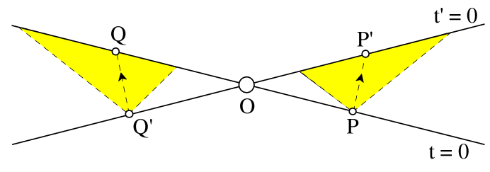
Figure 14: $O$ is the quantum horizon. Shaded regions are forwards lightcones. Signals from $P$ to $P^{\prime}$ and from $Q^{\prime}$ to $Q$ are shown with subluminal transmission speeds; this does not alter the overall conclusions.

It is clear from this diagram that the Lorentz transformation (123) leaves out much important information about how information can pass between the two frames, particularly in the case of genuine inter-frame experiments of the sort discussed here. Indeed, a much better physical description would be to regard $P$ and $Q^{\prime}$ as ESDs belonging to an initial Heisenberg net which sends signals to a subsequent Heisenberg net containing ESDs $P^{\prime}$ and $Q$. For each of these nets, their ESDs are scattered over some spacelike hypersurface in Minkowski spacetime, but neither hypersurface is associated with a single inertial frame. Note that ESDs $P$ and $Q$ are regarded as at rest in the same inertial frame, and similarly for $P^{\prime}$ and $Q^{\prime}$; there is therefore significant contextual information held by the observer which is not indicated in Figures $13$ and $14$ and cannot be ignored.

Some work has already been done on some issues related to entangled states and quantum horizons in such inter-frame experiments [41]. Our conclusions support the QDN view that it is not physically meaningful to talk about the preparation of quantum states, entangled or not, without reference to any context of subsequent observation. It is the choice of test apparatus which determines whether a state of an SUO should be regarded as entangled or not. For instance, in any discussion involving quantum information and black hole physics, problems will inevitably arise whenever quantum states are discussed without due regard for the equipment used to test them. For this reason, all discussions of quantum mechanics across event horizons or wavefunctions for the universe without due reference to observers and their equipment should be avoided. As we have shown above, it is insufficient even in SR to talk about Lorentz transformations without any reference to the apparatus involved in inter-frame experiments. When these are taken properly into account, the equations of special relativity have to be interpreted much more carefully and according to quantum principles.

PART IV: Commentary

It is our belief that the above examples demonstrate the viability of QDN as an alternative approach to QM. However, much remains to be done to establish further our intuition that QDN should be capable of doing everything that SQM can do and perhaps more. We are currently working our way through various other quantum optics experiments to confirm the viability and useful of our approach in that area. It is clear that at the one-photon level, the formalism gives an economical method of dealing with quite large scale networks. There may be problems with more complicated two-photon networks because the $X$ term in expression (27) vanishes only for sure when it is applied to the void state. However, a computer algebra approach would be able to deal with the complexities which arise on that score.

The QDN approach holds some promise of having applicability to other areas of quantum physics apart from quantum optics. We shall report developments in those area elsewhere. There are a number of points about QDN which it is appropriate to comment on here.

32 Hamiltonians and Lagrangians

SQM is generally characterized by the specification of a Hamiltonian operator, from which the dynamical evolution of state vectors can be determined. Frequently, such an operator is obtained from a classical model based on standard classical mechanical principles.

It will be evident from our review that there has been no mention of Hamiltonians or Lagrangians, so it looks as if that aspect of SQM has nothing in common with QDN. This would be a misleading deduction, however. Under those circumstances where there were many signal degrees of freedom in an experiment, and with an appropriate discussion of how discrete time could be represented in terms of a continuum approximation, we expect QDN can be made to look more like SQM, particularly in those cases where the rank of the Heisenberg net remains constant. Our discussion of path summations suggests that QDN should look like the conventional Feynman path integral formulation of SQM in the appropriate limits.

Hamiltonians and Lagrangians are just convenient ways of encoding acquired contextual information about a dynamical system, i.e., the previously discovered rules of the dynamics. The fact is that what matters in both SQM and QDN are the transition amplitudes. Once these are known, then either formalism should give good results. Where they differ is in how those amplitudes are obtained. SQM has certain standard procedures for obtaining the transition amplitudes from a given Hamiltonian or Lagrangian, such as evaluating path integrals or solving partial differential equations.

We regard Hamiltonians and the SQM formalism associated with them as useful weapons in the description of vast parts of the quantum universe, but there is no theorem which says that these are all the weapons we need. There might not be such a thing as a Hamiltonian or Lagrangian for the universe, the finding of which has been the dream of particle physicists for decades. What leads to our worry about such a concept is that in practice (i.e., as they are actually used), Hamiltonians are not absolute, but contextual. Each model requires its own Hamiltonian, and changes in the apparatus generally impose changes in that Hamiltonian, such as happens when external electromagnetic fields are introduced. The QDN view is that Hamiltonians arise only as and when the circumstances of an experiment dictate. In other words, a Hamiltonian without any associated concept of observation is a metaphysical concept with no physical value.

With the current state of development of QDN dynamics, we may need on occasion to use results from SQM in order to find correct expressions for semi-unitary operators in QDN. This should not be regarded as much different in principle to the use of classical mechanical Hamiltonians as templates for Hamiltonian operators SQM. The important point about our formalism is that it gives a different conceptual basis to the meaning of the calculations.

33 Quantum counterfactuality

Counterfactuals are true statements in classical logic, such as “$P$ implies $Q$”, made under the circumstance that it is known that the premise $P$ is in fact false. Counterfactuals are widely used in ordinary life and form the basis of the classical world view, but they should be treated with great care or avoided when in comes to discussions of quantum processes. In the classical world view, things which did not, or could not, happen are sometimes assigned significance and truth values which they do not merit. For example, the classical world view would circumvent Heisenberg’s uncertainty principle with an argument such as the following: “We have just measured the position of this particle with absolute precision. However, if we had chosen instead to measure its momentum, we would have established that dynamical variable with absolute precision. Therefore, this proves that a particle can have precise position and precise momentum simultaneously.”

We call the principle that “if something has not been observed, then it is irrelevant” the Heisenberg-Peres principle, or quantum counterfactuality. QDN adheres to quantum counterfactuality by a strict adherence to the basic principle that only what the observer knows and does with their apparatus has significance. This has bearing on the old debate between the block universe model of spacetime and the process time view. QDN is committed to the latter. Real observers exist as one-off processes in the physical universe, and their experiments are run serially in process time. Given unique information, there is only one preferred basis associated with any given apparatus, and it is not permitted to discuss other bases as if they had physical significance without explaining carefully what this might mean. This requires acknowledging the use of counterfactuals, and brings us to the next point, the issue of symmetries.

34 Quantum symmetries

SQM makes great use of symmetry arguments, involving such symmetries as rotational and translational invariance, as if the associated transformations could be done at any time. Such arguments are usually vindicated retrospectively by the results obtained in the laboratory, but it has to be pointed out that in general, there are invariably a number of hidden assumptions left unstated in such discussions. These invariably clash with what actually happens in the laboratory. Any given individual run of an experiment involves only one realization of the apparatus, and generally, observers cannot change their apparatus in the middle of a run without a great deal of physical consequences. For example, in a Stern-Gerlach experiment, the main magnetic field has to lie in one direction only. If the outcomes of other runs with the magnetization axis lying along different directions are related by symmetries, then clearly what is involved are comparisons of outcomes of different apparatus at different times and places. This will in general involve the use of counterfactuals in a way consistent with quantum principles. We do not have the space to comment on this point further, save to say that it is our belief that QDN principles provide a sound basis for such discussions.

35 Final comments

Our experience with the formalism described here leads us to have some confidence that it has more useful things to say about quantum physics than discussed here. It gives a different perspective on the significance of quantum amplitudes and allows for a wider form of discussion than is usual in SQM. We have had no opportunity here to discuss some important topics such as mixed states or what a physically correct approach to “quantum gravity” might involve, save to say that in both cases, we envisage a true novelty: uncertainty about the actual apparatus and not just about its labstates [42]. What this means is that at a given time, an observer might not know for sure what sort of Heisenberg net they would be using in the future, and could give only probability estimates for a range of possibilities. It is our intuition that the real world, in which observers and apparatus themselves are created and destroyed by dynamical processes, might be modelled one day by some enhanced version of quantized dynamical networks.

References

- [1] I thank Dr. K. K. Phua of World Scientific for sending me a review and reprint of Feynman’s doctoral thesis, viz., L. M. Brown, Feynman’s Thesis, A new Approach to Quantum Theory, World Scientific (2005), from which the above quotation is taken.
- [2] M. Born, Z. Physik 38, 803–827 (1926).
- [3] M. Born, The statistical interpretation of quantum mechanics, Nobel prize lecture, (1954), published by World Scientific in Nobel Lectures: Physics 1901-1995. I am indebted to Dr. K. K. Phua of World Scientific for generously sending me this CD.
- [4] H. J. Maris, J. Low Temp. Phys., 120, 173-204 (2000).
- [5] D. Deutsch, The Fabric of Reality, The Penguin Press (1997).
- [6] W. H. Zurek Los Alamos Science 27, 2–24 (2002).
- [7] G. Jaroszkiewicz, The running of the Universe and the quantum structure of time, arXives:quant-ph/0105013 (2001).
- [8] J. Eakins, Classical and Quantum Causality in Quantum Field Theory, or The Quantum Universe, Ph.D. Thesis, University of Nottingham (2004).
- [9] J. Eakins and G. Jaroszkiewicz, A Quantum Computational Approach to the Quantum Universe, in New Developments in Quantum Cosmology Research, edited by Albert Reimer, Horizons in World Physics 247 (Nova Science Publishers, Inc. New York, 2005).
- [10] H. Paul, Introduction to Quantum Optics, CUP (2004).
- [11] G. Jaroszkiewicz, Quantum register physics, arXives:quant-ph/0409094 (2004).
- [12] G. Jaroszkiewicz and J. Ridgway-Taylor, Int. J. Mod. Phys. B, 20 (11-13) 1382-1389 (2006).
- [13] W. Heisenberg, Z. Physik A 33(1) 879 – 893 (1925).
- [14] E. Schrodinger, Ann. Phys. Leipzig, 79, 361–376 (1926).
- [15] G. Jaroszkiewicz and J. Ridgway-Taylor, Quantum computational representation of the bosonic oscillator, arXives:quant-ph/0502166 (2005).
- [16] J. Ridgway-Taylor, Elements of Classical and Quantum Theories from Classical and Quantum Bits, Ph.D. Thesis, University of Nottingham (2007).
- [17] M. Planck, Verhandl. Dtsch. Phys. Ges. 2, 202-204 (1900).
- [18] N. Bohr, Phil. Mag. 26, 1–25 (1913).
- [19] W. Heisenberg, Z. Physik 43, 172–198 (1927).
- [20] D. Bohm, Phys. Rev. 85, 166-193 (1952).
- [21] J. von Neumann, The Mathematical Foundations of Quantum Mechanics, Princeton University Press (1955).
- [22] A. Peres, Quantum Theory: Concepts and Methods, Kluwer Academic Publishers (1993).
- [23] E. Mach, Die Mechanik in Ihrer Entwicklung Historisch-Kritisch Dargestellt (1912), English translation by T. J. McCormack, “The Science of Mechanics”, Open Court, La Salle, Ill.
- [24] H. Everett III, Rev. Mod. Phys.,
- [25] P. Jordan and E. P. Wigner, Z. Physik, 47, 631–651 (1928).
- [26] J. D. Bjorken and S. D. Drell, Relativistic Quantum Fields, McGraw-Hill Inc (1965).
- [27] B. Schutz, Geometrical Methods of Mathematical Physics, Cambridge University Press (1980).
- [28] B. Misra and E. C. G. Sudarshan, J. Math. Phys. 18, 756-763 (1977).
- [29] K. Gödel, Rev. Mod. Phys., 21 (3), 447-450 (1949).
- [30] J. Schwinger, Particles and Sources, Gordon and Breach (1969).
- [31] R. P . Feynman and A. R. Hibbs, Quantum Mechanics and Path Integrals, McGraw-Hill, New York (1965).
- [32] A. Zeilinger, Am. J. Phys. 49(9), 882-883 (1981).
- [33] R. J. Eden, P. V. Landshoff, D. I. Olive and J. C. Polkinghorne, The Analytic S-Matrix, CUP (1966).
- [34] H. E. Brandt, Am. J. Phys., 67, 434-439 (1999).
- [35] H. E. Brandt, Quantum Measurement with a Positive Operator-Valued Measure, Proceedings of the Wigner Centennial Conference, Pecs, Hungary (2002).
- [36] A. Einstein, B. Podolsky and N. Rosen, Phys. Rev. 47, 777-780 (1935).
- [37] M. A. Horne, A. Shimony and A. Zeilinger, Phys. Rev. Lett., 62 (19) 2209-2212 (1989).
- [38] G. Jaroszkiewicz and J. Eakins, Particle decay processes, the quantum Zeno effect and the continuity of time, arXives:quant-ph/0608248 (2006).
- [39] J. J. Bollinger et al., Phys. Rev. A 41(5) 2295-2300 (1990).
- [40] L. de Broglie, Recherches sur la Théorie Des Quanta, Ph.D thesis, Faculty of Sciences at Paris University (1924).
- [41] G. Jaroszkiewicz, Proposed split-causality test of the relativity principle, arXives:gr-qc/0612082 (2006).
- [42] G. Jaroszkiewicz, The Entropy of the Future, Endophysics, Time, Quantum and the Subjective, edited by R. Buccheri et al, World Scientific (2005).