Spin-orbital effects in magnetized quantum wires and spin chains

Abstract

We present analysis of the interacting quantum wire problem in the presence of magnetic field and spin-orbital interaction. We show that an interesting interplay of Zeeman and spin-orbit terms, facilitated by the electron-electron interaction, results in the spin-density wave (SDW) state when the magnetic field and spin-orbit axes are orthogonal. We show that this instability is enhanced in a closely related problem of Heisenberg spin chain with asymmetric uniform Dzyaloshinskii-Moriya (DM) interaction. Magnetic field in the direction perpendicular to the DM anisotropy axis results in staggered long-range magnetic order along the orthogonal to the applied field direction. We explore consequences of the uniform DM interaction for the electron spin resonance (ESR) measurements, and point out that they provide way to probe right- and left-moving excitations of the spin chain separately.

I Introduction

Over the last several years there has been a remarkable growth in research activity in the field of spintronics with the ultimate goal to fabricate novel spin-filter devices which can control and manipulate the electron spins datta . The proposals for such a spin-filter device contains two achievable attributes, a ballistic quantum wire and the presence of a tunable Rashba spin-orbit coupling responsible for controlling the electron spin. Ballistic quantum wires are created in a 2DEG by cleaved edge over growth, whereas the Rashba effect arises due to the asymmetry associated with the confinement potential rashba . The asymmetry and hence the Rashba coupling strength can be controlled by applying the gate voltage. Although the role of spin-orbital and magnetic (Zeeman) fields in the electric and spin transport is well understood for a non-interacting quantum wire moroz ; streda ; levitov ; pereira ; halperin , the case of interacting electrons remains the subject of active research kimura96 ; samokhin00 ; hausler01 ; iucci03 ; governale04 ; yu04 ; gritsev05 ; hyunlee05 ; hikihara05 .

It should be noted that finite spin-orbit coupling is very natural, and, strictly speaking, unavoidable, in semiconducting quantum wires due to pronounced structural asymmetry inherent in the fabrication process. Also, in addition to the noted asymmetry of confining potentials (which include quantum-well potential that confines electrons to a 2D layer as well as transverse [in-plane] potential that forms the one-dimensional channel moroz ), spin-orbit interaction is inherent to semiconductors of either zinc-blende or wurtzite lattice structures lacking inversion symmetry dresselhaus .

Another very interesting system that motivates our investigation is provided by one-dimensional electron surface states on vicinal surface of gold vicinal-au as well as by electron states of self-assembled gold chains on stepped Si$(111)$ surface of silicon himpsel06 . In both of the systems one-dimensional ballistic channels appear due to atomic reconstruction of surface layer of atoms, see also mugarza03 ; ortega05 . The resultant surface electronic states lie within the bandgap of bulk states, and thus, to high accuracy, are decoupled from electrons in the bulk. Spin-orbit interaction is unexpectedly strong in these systems, with the spin-orbit energy splitting of the order of $100$ meV. In fact, spin-split subbands of Rashba type have been observed in angular resolved photoemission spectroscopy (ARPES) in both two-dimensional lashell and one-dimensional settings vicinal-au ; himpsel06 . The very fact that the two (horizontally) spin-split parabolas are observed in ARPES speaks for high quality and periodicity of the obtained surface channels.

As we show below, the most interesting situation involves electrons subjected to both spin-orbital and magnetic fields. While it is perhaps impractical to think of ARPES measurements in the presence of magnetic field, it is quite possible to imagine experiments on magnetic metal surfaces krupin05 ; dedkov08 . It is then natural to investigate combined effect of non-commuting spin-orbit and Zeeman interactions, together with electron-electron interaction, on the one-dimensional system of electrons.

Electrons in a quantum wire (or, in a one-dimensional surface channel) are a good realization for a Tomonaga-Luttinger liquid and serves as an ideal system for the study of the interplay of magnetic field and Rashba spin-orbit effect on the interacting quantum wire. The magnetic field breaks the time-reversal symmetry of the Hamiltonian and splits the band of free electrons into two, corresponding to up-spin and down-spin electrons, reducing spin-rotational symmetry of the system from SU(2) to U(1). Subsequent inclusion of the Rashba term, $H_{R}\propto\vec{\sigma}\times\vec{p}\cdot\hat{z}$, see Eq.(2), breaks this U(1) symmetry (observe that $[\sigma_{z},H_{R}]\neq 0$). In addition, the spin-orbit interaction (SOI) $H_{R}$ breaks spatial inversion symmetry ${\cal P}:x\to-x$. A consequence of the fully broken SU(2) symmetry is the generation of new scattering processes which are no longer spin-conserving. These are the Cooper scattering processes in which a pair of electrons in the lower band scatter to the upper band and vice versa sun07 . A relevant Cooper term creates a gap in the energy spectrum leading to a long range spin-density wave order. We find that the gap strength is proportional to the backscattering ($2k_{F}$ component) of the electron-electron interaction potential and the ratio of the Rashba to the Zeeman energy. For a large enough gap the ordering in the spin-density wave can crucially suppress the backscattering process of electrons from an isolated impurity. Brief description of our main results was previously given in Ref. sun07, .

We will also analyze an alternate system, a Mott-Hubbard Heisenberg spin-1/2 chain, in the presence of magnetic field and Dzyloshinskii-Moriya (DM) interaction. A magnetic field applied at an angle perpendicular to the DM anisotropy axis breaks the continuous U(1) symmetry and consequently a true long range order can develop in the spin-chain. The case of a staggered DM term has been studied experimentally dender97 and theoretically ao , and has been shown to open up a gap in the spectrum with the gap scaling as $B^{2/3}$ with the magnetic field $B$. The case of a uniform DM term is also experimentally relevant, see for example Ref.zakharov06, , but has not been discussed much theoretically. We will show that the case of a uniform DM term and perpendicular magnetic field can be described analogously to the quantum wire in the presence of spin-orbit interaction and magnetic field.

The outline for the paper is as follows: In Sec.II we will review non-interacting electrons in the presence of magnetic field and Rashba spin-orbit term. We then consider interaction effects by using standard bosonization approach. In Sec.III.2 we will perform renormalization group analysis to determine relevant and irrelevant terms. In Sec.IV we use perturbative approach to generate relevant terms. The role of relevant terms on the transport property of electrons in the presence of a single impurity is analyzed in section V. In Sec.VI, we consider a spin-$1/2$ Heisenberg antiferromagnetic chain in the presence of magnetic field and uniform DM term and compare this system with the quantum wire. Comparison with the case of a staggered DM term is considered in Sec.VI.4. In Section VII we discuss the role ESR measurements can play in unraveling the DM term in the spin chain. Technical details of our calculations are described in Appendices.

II 1D Electrons in the presence of magnetic field and Rashba spin orbit term

The Hamiltonian for an electron subject to the Rashba spin-orbit term and in the presence of magnetic field is given by

$$H_{0} = \frac{\hbar^{2}(p^{2}_{x}+p^{2}_{y})}{2m}+V(x)-g\mu_{B}\frac{\vec{\sigma}}{2}\cdot\vec{B}+H_{R},$$ (1)

$$H_{R} = \frac{\alpha_{R}}{\hbar}(\sigma_{x}p_{y}-\sigma_{y}p_{x})$$ (2)

where $\alpha_{R}$ is the Rashba spin-obrit coupling, $g$ is the effective Bohr magneton, $B$ is the magnetic field, $\sigma_{\mu}$ ($\mu=x,y,z)$ are the Pauli matrices and the potential $V(x)=m\omega^{2}x^{2}/2$ typically confines the particle in the $x-$direction. When the confining potential is strong enough so that the width of the wire $\sqrt{\hbar/(2m\omega)}$ is much smaller than the electron Fermi-wavelength, only the first sub-band is occupied and the Hamiltonian (1) acquires a one-dimensional form

$$H_{0}\approx\frac{\hbar^{2}k^{2}}{2m}+\frac{\alpha_{R}}{\hbar}(\sigma_{x}k)-g\mu_{B}\frac{\vec{\sigma}}{2}\cdot\vec{B}.$$ (3)

Here and below $k$ is electron’s momentum along the axis of the wire, which we will denote as $x$-axis in the following for notational convenience. We also set $\hbar=1$.

It is easy to see that in the absence of magnetic field SOI in (3) can be easily gauged away via the spin-dependent shift of the momentum, $H_{0}(B=0)\propto(k+m\alpha_{R}\sigma_{x})^{2}$. Corrections arising from the omitted term $\alpha_{R}\sigma_{y}p_{x}$ (2) produce small spin-dependent variations of the velocities of right- and left-moving particles samokhin00 . These, however, are not important for our purposes for as long as $\alpha_{R}k_{F}\ll E_{F}$, which is the limit (along with $\Delta_{Z}\ll E_{F}$) considered in this work. With interactions included, electrons form Luttinger liquid with somewhat modified critical exponents, in comparison with the standard case of no SOI samokhin00 ; iucci03 .

Most interesting situation arises when both SOI and Zeeman terms are present simultaneously and do not commute with each other as happens when spin-orbital axis ($\sigma_{x}$ in (3)) is different from the magnetic field direction. In what follows we choose magnetic field to point along the $z-$direction, $\vec{B}=B\hat{z}$. The energy eigenvalues of the Hamiltonian (3) is found as levitov ; pereira

$$\epsilon_{\pm}=\frac{k^{2}}{2m}\pm\sqrt{(\alpha_{R}k)^{2}+(\frac{\Delta_{z}}{2})^{2}},$$ (4)

and the momentum dependent eigen-spinors are, for $\epsilon_{+}(k)$:

$$|\chi_{+}(k)\rangle\equiv\left[\begin{array}[]{cc}\sin\frac{\gamma(k)}{2}\\ \cos\frac{\gamma(k)}{2}\end{array}\right],$$ (7)

and for $\epsilon_{-}(k)$:

$$|\chi_{-}(k)\rangle\equiv\left[\begin{array}[]{cc}\cos\frac{\gamma(k)}{2}\\ -\sin\frac{\gamma(k)}{2}\end{array}\right],$$ (10)

where $\Delta_{z}=g\mu_{B}B$ and rotation angle $\gamma(k)$ is introduced

$$\gamma(k)=\arctan\frac{2\alpha_{R}k}{\Delta_{z}}.$$ (11)

Notice that particles with momentum $\pm k$ experiences an effective magnetic field $\vec{B}_{\rm eff}=\mp 2\alpha_{R}k/(g\mu_{B})\hat{x}+B\hat{z}$, thus spin directions in each band varies with the momentum. Going from left to the right side of the band, the spins ”rotate” along the counter-clockwise direction. At $k=0$, the effective magnetic field is just the applied field, thus the separation between the two bands is minimum and the spins align according to the applied field, i.e., along the $\mp z-$direction. For states with the same energy the spin states of $+$ and $-$ bands are no longer orthogonal if there is a finite magnetic field and Rashba spin-orbit coupling. In particular the right and left Fermi levels satisfy the following property

$$k_{-}^{R/L}+k_{+}^{R/L}\approx\pm 2k_{F}$$ (12)

and

$$\delta k_{F}=|k_{-}^{R/L}-k_{+}^{R/L}|\approx\frac{m}{k_{F}}\sqrt{(2k_{F}\alpha_{R})^{2}+(\Delta_{z})^{2}}.$$ (13)

The magnitude of velocities at the Fermi level are

$$|u_{\pm}|\approx v_{F}\mp\frac{(\Delta_{z})^{2}}{2k_{F}\sqrt{4(\alpha_{R}k_{F})^{2}+(\Delta_{z})^{2}}},$$ (14)

where $v_{F}=k_{F}/m$. The spin overlap between the upper ($+$) and lower ($-$) band is non-zero,

$$\langle\chi(k_{+}^{R/L})|\chi(k_{-}^{R/L})\rangle=\sin\frac{\gamma(k_{+}^{R/L})-\gamma(k_{-}^{R/L})}{2}.$$ (15)

As will be discussed in the next section, the non-orthogonality of the spin-states acquires important consequences when one turns on the electron-electron interactions.

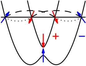
Figure 1: Occupied subbands $\epsilon_{\pm}$ of Eq. 4. Arrows illustrate spin polarization in different subbands. Dashed (dotted) lines indicate exchange (direct) Cooper scattering processes.

III Intersubband Interaction Effects

The interaction part in terms of the particle-field operators $\Psi_{\sigma}(x)$ and $\Psi^{\dagger}_{\sigma}(x)$ ( $\sigma$ and $\sigma^{\prime}$ are the spin indices) is given by

$$H_{\text{int}}=\frac{1}{2}\int dxdx^{\prime}U(x-x^{\prime})\Psi_{\sigma}^{\dagger}(x)\Psi_{\sigma^{\prime}}^{\dagger}(x^{\prime})\Psi_{\sigma^{\prime}}(x^{\prime})\Psi_{\sigma}(x),$$ (16)

where the summation on pairs of identical spin indices is assumed and $U(x-x^{\prime})$ is the screened (by surrounding gates) interaction between the electrons. The field $\Psi_{\sigma}(x)$ is conventionally defined in terms of the annihilation operator $a_{\sigma}(k)$ of a free particle in the state $e^{ikx}$ and with spin $\sigma=\uparrow,\downarrow$: $\Psi_{\sigma}(x)=\int\frac{dk}{2\pi}e^{ikx}a_{\sigma}(k)$. Alternatively, annihilation operators $a_{\pm}(k)$ of particles which are the eigen-states of the Hamiltonian (1) with eigen-energies $\epsilon_{\pm}(k)$, can be used to represent the field operator as follows:

$$\Psi_{\sigma}(x)=\sum_{\nu=\pm}\int\frac{dk}{2\pi}e^{ikx}\langle\chi_{\nu}(k)|\sigma\rangle a_{\nu}(k).$$ (17)

The low energy physics of the interacting wire is described by linearizing the spectrum near the Fermi-points, $\pm k_{\pm}$. The $\sigma=\uparrow,\downarrow$ field operators are now described, in coordinate space, in terms of the chiral right ($R_{\nu}$) and left ($L_{\nu}$) movers of $\nu=\mp$ subbands as follows

$$\Psi_{\sigma}(x)=\sum_{\nu=\mp}\langle\chi_{\nu}(k_{\nu})|\sigma\rangle e^{ik_{\nu}x}R_{\nu}+\langle\chi_{\nu}(-k_{\nu})|\sigma\rangle e^{-ik_{\nu}x}L_{\nu}.$$ (18)

Following review , we decompose the interaction part of the Hamiltonian (16) into intra-subband $H_{\text{intra}}$ and inter-subband $H_{\text{inter}}$ scattering processes. The intra-subband process, $H_{\text{intra}}$, describes the interaction between electrons in the same subband and involves the standard forward and backscattering processes, see Appendix A. The second scattering mechanism, $H_{\text{inter}}$, involves scattering between electrons in different subbands and can be conveniently divided into forward, backward and Cooper scattering processes. Below we will discuss the inter-subband scattering processes in more detail. The forward scattering process involves interaction between $q\approx 0$ components of the densities in the two subbands

$$H_{\text{inter}}^{\text{F}}=\frac{1}{2}U(0)\int dx\sum_{\nu=\pm}(R^{\dagger}_{\nu}R_{\nu}+L^{\dagger}_{\nu}L_{\nu})$$

$$\times(R^{\dagger}_{-\nu}R_{-\nu}+L^{\dagger}_{-\nu}L_{-\nu}).$$ (19)

The inter-subband backscattering process is classified into direct and exchange scattering. Direct backscattering process involves $q\approx 2k_{\pm}$ components of the densities in the two subbands: a left (right) moving electron in the subband $\nu$ ($-\nu$) changes its direction to become a right (left) moving one while remaining in the same band,

$$H_{\text{inter}}^{\text{d-B}}=\cos[\gamma(k_{+})]\cos[\gamma(k_{-})]U(k_{+}+k_{-}){}$$

$$\times\sum_{\nu=\pm}\int dx~{}e^{i2(k_{\nu}-k_{-\nu})x}(R^{\dagger}_{\nu}L_{\nu})(L^{\dagger}_{-\nu}R_{-\nu}).$$ (20)

This contribution involves an oscillatory factor $\exp[i2(k_{\nu}-k_{-\nu})x]$ in the integral due to the non-conservation of momentum during the scattering.

The other backscattering process is via a momentum conserving exchange mechanism, where electrons again scatter by large momentum transfer and in the process exchange their bands. The scattering channel conserves momentum and reads

$$H_{\text{inter}}^{\text{ex-B}}=\frac{1}{2}\sum_{\nu=\pm}\Big{\{}U(k_{\nu}-k_{-\nu})\sin^{2}[\frac{\gamma(k_{\nu})-\gamma(k_{-\nu})}{2}]$$

$$\times\int dx\Big{(}(R^{\dagger}_{\nu}R_{-\nu})(R^{\dagger}_{-\nu}R_{\nu})+(L^{\dagger}_{\nu}L_{-\nu})(L^{\dagger}_{-\nu}L_{\nu})\Big{)}{}$$

$$+2U(k_{\nu}+k_{-\nu})\sin^{2}[\frac{\gamma(k_{\nu})+\gamma(k_{-\nu})}{2}]$$

$$\times\int dx(R^{\dagger}_{\nu}L_{-\nu})(L^{\dagger}_{-\nu}R_{\nu})\Big{\}}.$$ (21)

Note the appearance of (squared) wave function overlap factors, $\propto\langle\chi(k_{\nu})|\chi(\pm k_{-\nu})\rangle$, which signify the exchange nature of the scattering. Note also that these factors are non-zero due to a finite Rasbha coupling $\alpha_{R}$, which allows electrons to scatter without conserving their spins.

The Cooper scattering process, which is central to our story, involves scattering of a pair of opposite movers (right and left) in the subband $\nu$ into a similar pair in the other, $-\nu$, subband. Each pair has zero total momentum which remains conserved in this scattering. Being pair-tunneling like, Cooper scattering requires non-conservation of spin. It represents, for example, a scattering of a pair of two (almost) down-spin electrons into a pair of two (almost) up-spin ones. The Cooper scattering reads

$$H_{\text{inter}}^{\text{C}}=\int dx\Big{\{}U(k_{-}-k_{+})\sin^{2}[\frac{\gamma(k_{-})-\gamma(k_{+})}{2}]$$

$$-U(k_{-}+k_{+})\sin^{2}[\frac{\gamma(k_{-})+\gamma(k_{+})}{2}]\Big{\}}$$

$$\times(R^{\dagger}_{-}L^{\dagger}_{-}R_{+}L_{+}+\text{h.c.}).$$ (22)

The first term (direct Cooper scattering) is due to electrons in the band $R_{\nu}$ and $L_{\nu}$ jumping into $R_{-\nu}$ and $L_{-\nu}$, respectively. The coefficient for this term is $\propto U(\delta k_{F})\sin^{2}[(\gamma_{-}-\gamma_{+})/2]$, where $\delta k_{F}=|k_{\nu}-k_{-\nu}|$ is the momentum transfer for an electron and $\sin^{2}[(\gamma_{-}-\gamma_{+})/2]$ is the squared overlap integral. (For brevity, we denote $\gamma(k_{\pm})=\gamma_{\pm}$ here and in the following.) The second process (exchange) with electron scattering from $R_{\nu}$ and $L_{\nu}$ to $L_{-\nu}$ and $R_{-\nu}$, respectively, involves a coefficient, $\propto U(k_{\nu}+k_{-\nu})\sin^{2}[(\gamma_{-}+\gamma_{+})/2]$, with a larger, $\sin^{2}[(\gamma_{-}+\gamma_{+})/2]$, overlap integral. The bigger overlap for this second ($R_{\nu}\leftrightarrow L_{-\nu}$) process is also rather clear from pictorial representation of spin orientation in different subbands, as shown in Fig. 1. For the case of short-ranged (screened) interaction potential a simple estimate, using (12) and (13),

$$\frac{U(k_{-}-k_{+})\sin^{2}[\frac{\gamma_{-}-\gamma_{+}}{2}]}{U(k_{-}+k_{+})\sin^{2}[\frac{\gamma_{-}+\gamma_{+}}{2}]}\approx\frac{U(\delta k_{F})}{U(2k_{F})}\Big{(}\frac{\Delta_{z}}{2E_{F}}\Big{)}^{2}\ll 1$$ (23)

shows that the second, exchange Cooper process, dominates. This defines the regime to be considered in this work.

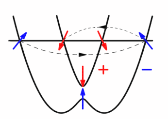
Figure 2: Asymmetric back-scattering processes.

Finally we take into account two classes of momentum non-conserving scattering processes where one of them exhibits mixed features of Cooper and back-scattering (called as asymmetric back-scattering process) while the other one has features reminiscent of Cooper and forward scattering processes ( asymmetric forward-scattering process). A typical asymmetric back (forward) scattering event involves total momentum change $\pm\delta k_{F}$, see Fig.2. For example, right and left moving fermions in the same sub-band scatter into left (right) and right (left) moving fermions respectively, with one of the fermions now in a different sub-band. Alternatively, the oppositely moving fermions may be in different sub-bands to begin with but end up in the same sub-band with opposite (same) momentums. The scattering process acquires a slowly (compared to direct back scattering (20)) oscillating factor $\exp[i(k_{\nu}-k_{-\nu})x]$ owing to the non-conservation of momentum and is given by

$$~{}~{}~{}~{}~{}~{}H_{\text{asymm}}=\sin(\frac{\gamma_{+}+\gamma_{-}}{2})\sum_{\nu=\pm}\text{sgn}(\nu)U(2k_{F})\cos(\gamma_{\nu})\times$$

$$\int dx[e^{i(k_{\nu}-k_{-\nu})x}(R^{\dagger}_{\nu}L^{\dagger}_{\nu}R_{\nu}L_{-\nu}-R^{\dagger}_{-\nu}L^{\dagger}_{\nu}R_{\nu}L_{\nu})+\text{h.c.}].$$ (24)

The above expression reflects contributions from only the asymmetric back-scattering processes. The asymmetric forward-scattering processes involve identical fermion operators as in Eq.(24). However the ratio of amplitudes for asymmetric forward to asymmetric back-scattering process is small,

$$\frac{U(\delta k_{F})\sin[\frac{\gamma_{\nu}-\gamma_{-\nu}}{2}]}{U(2k_{F})\sin{[\frac{\gamma_{\nu}+\gamma_{-\nu}}{2}]}\cos{\gamma_{\nu}}}\approx\frac{U(\delta k_{F})}{U(2k_{F})}\frac{\sqrt{\Delta_{z}^{2}+4(\alpha_{R}k_{F})^{2}}}{2E_{F}}\ll 1,$$

which allows us to neglect contributions from asymmetric forward-scattering processes altogether.

The electron density in the quantum wire is assumed to be incommensurate with the lattice spacing, hence the Umklapp scattering process is not considered. To summarize, the interaction part of the Hamiltonian has been decomposed in terms of three broadly defined scattering processes, intra subband, inter subband and asymmetric scattering process,

$$H=H_{\text{intra}}+H_{\text{inter}}+H_{\text{Asymm}}.$$ (25)

III.1 Bosonization

Bosonization is performed by expressing the fermionic operators in the Hamiltonian via the chiral bosonic $\phi_{R/L_{\nu}}$ fields gnt-book ; giamarchi-book ; hubbard-ladder . The fermionic fields in terms of the chiral bosonic field are as follows

$$R_{\pm}=\frac{\eta_{\pm}}{\sqrt{2\pi a_{0}}}e^{i\sqrt{4\pi}\phi_{R\pm}},\ \ L_{\pm}=\frac{\eta_{\pm}}{\sqrt{2\pi a_{0}}}e^{-i\sqrt{4\pi}\phi_{L\pm}},$$ (26)

where $a_{0}\sim k_{F}^{-1}$ is the short distance cutoff and $\eta_{\pm}$ are the Klein factors which are introduced to ensure the correct anti-commutation relations for the fermionic operators from different ($\pm$) subbands. The bosonic operators obey the following commutation relations:

$$[\phi_{R\nu},\phi_{L\nu^{\prime}}]=\frac{i}{4}\delta_{\nu\nu^{\prime}};\ \ \ \text{where}\ \ \ \nu,\nu^{\prime}=\pm$$ (27)

$$[\phi_{R/L\nu}(x),\phi_{R/L\nu^{\prime}}(y)]=\pm\frac{i}{4}\delta_{\nu\nu^{\prime}}\text{sign}(x-y),$$ (28)

the first of which, (27), ensures anticommutation between right and left movers from the same subband, while the second is needed for the anticommutation between like species (i.e. right with right, left with left). Klein factors anticommute

$$\{\eta_{\nu},\eta_{\nu^{\prime}}\}=2\delta_{\nu\nu^{\prime}}~{},~{}\eta_{\nu}^{\dagger}=\eta_{\nu}.$$ (29)

In the following we choose the gauge where $\eta_{+}\eta_{-}=i$. The chiral $\phi_{R/L\nu}$ are expressed in terms of $\phi_{\nu}$ and its dual $\theta_{\nu}$ as follows

$$\phi_{R\nu}=\frac{\phi_{\nu}-\theta_{\nu}}{2};\ \ \phi_{L\nu}=\frac{\phi_{\nu}+\theta_{\nu}}{2},$$ (30)

The bosonized form of the Hamiltonian is obtained by making use of equations (26) through (30), as well as the following results for (chiral) densities

$$R^{\dagger}_{\nu}R_{\nu}=\frac{\partial_{x}\phi_{R\nu}}{\sqrt{\pi}}=\frac{\partial_{x}(\phi_{\nu}-\theta_{\nu})}{\sqrt{4\pi}},{}$$

$$L^{\dagger}_{\nu}L_{\nu}=\frac{\partial_{x}\phi_{L\nu}}{\sqrt{\pi}}=\frac{\partial_{x}(\phi_{\nu}+\theta_{\nu})}{\sqrt{4\pi}}$$ (31)

The (bosonized) Hamiltonian in terms of $\phi_{\nu}$ and $\theta_{\nu}$ is the sum of intra-subband, inter-subband scattering and asymmetric scattering processes,

$$H=H_{\text{intra}}+H_{\text{inter}}+H_{\text{asymm}},$$ (32)

where the intra-subband part has the usual form (see Appendix A)

$$H_{\text{intra}}=\frac{1}{2}\sum_{\nu=\pm}\int dx\Big{\{}v_{F}(\partial_{x}\theta_{\nu})^{2}{}$$

$$+(v_{F}+\frac{U(0)-\cos^{2}[\gamma(k_{\nu})]U(2k_{\nu})}{\pi})(\partial_{x}\phi_{\nu})^{2}\Big{\}}.$$ (33)

The inter-subband part of the Hamiltonian, $H_{inter}$, is given by

$$H_{\text{inter}}=H_{\text{inter}}^{\text{F}}+H_{\text{inter}}^{\text{d-B}}+H_{\text{inter}}^{\text{ex-B}}+H_{\text{inter}}^{\text{C}},$$ (34)

where

$$H_{\text{inter}}^{\text{F}}=\frac{U(0)}{\pi}\int dx~{}\partial_{x}\phi_{+}\partial_{x}\phi_{-},{}$$

$$H_{\text{inter}}^{\text{d-B}}=\frac{U(2k_{F})\cos^{2}[\gamma_{F}]}{2(\pi a_{0})^{2}}{}$$

$$\times\int dx\cos[2\sqrt{\pi}(\phi_{-}-\phi_{+})+2(k_{+}-k_{-})x],{}$$

$$H_{\text{inter}}^{\text{ex-B}}=-\frac{U(2k_{F})}{2\pi}\sin^{2}[\gamma_{F}]{}$$

$$\times\int dx~{}(\partial_{x}\phi_{+}\partial_{x}\phi_{-}-\partial_{x}\theta_{+}\partial_{x}\theta_{-}),{}$$

$$H_{\text{inter}}^{\text{C}}=\frac{U(2k_{F})\sin^{2}[\gamma_{F}]}{2(\pi a_{0})^{2}}{}$$

$$\times\int dx\cos[2\sqrt{\pi}(\theta_{-}-\theta_{+})].$$ (35)

The asymmetric part has the following bosonized form,

$$H_{\text{asymm}}=-\frac{\sqrt{2}U(2k_{F})\sin(2\gamma_{F})}{(2\pi)^{3/2}a_{0}}\int dx\{\partial_{x}(\phi_{R-}-\phi_{R+}){}$$

$$\times\sin[\sqrt{4\pi}(\phi_{L-}-\phi_{L+})-\delta k_{F}x]+\partial_{x}(\phi_{L-}-\phi_{L+}){}$$

$$\times\sin[\sqrt{4\pi}(\phi_{R-}-\phi_{R+})-\delta k_{F}x]\}.$$ (36)

In deriving Eqs. (35) and (36) we took limits $\Delta_{z}\ll E_{F}=v_{F}k_{F}$ and $\alpha_{R}k_{F}\ll E_{F}$ which allowed us to neglect velocity differences (14) in the two subbands and approximate $U(2k_{\pm}),U(\frac{3k_{\nu}-k_{-\nu}}{2})\approx U(2k_{F})$ and $\gamma(k_{\pm})\approx\gamma(k_{F})\equiv\gamma_{F}$. An important exception to this replacement is provided by $H_{\text{inter}}^{\text{d-B}}$ and $H_{\text{asymm}}$ in (35) and (36), respectively, where momentum mismatch factors $2(k_{-}-k_{+})x=2\delta k_{F}x$ and $(k_{-}-k_{+})x=\delta k_{F}x$ must be preserved. It is worth noting here that the approximations assumed do not restrict the ratio $2\alpha_{R}k_{F}/(g\mu_{B}B)=E_{\text{s-o}}/\Delta_{z}$, which can still take on any value.

A more standard representation of the Hamiltonian is in terms of the symmetric $\phi_{\rho}$, $\theta_{\rho}$ (charge) and anti-symmetric $\phi_{\sigma}$, $\theta_{\sigma}$ (spin) modes. These combinations are defined as follows

$$\varphi_{\rho}=\frac{\phi_{-}+\phi_{+}}{\sqrt{2}},\ \ \varphi_{\sigma}=\frac{\phi_{-}-\phi_{+}}{\sqrt{2}},{}$$

$$\theta_{\rho}=\frac{\theta_{-}+\theta_{+}}{\sqrt{2}},\ \ \ \theta_{\sigma}=\frac{\theta_{-}-\theta_{+}}{\sqrt{2}}.$$ (37)

The Hamiltonian now reads

$$H=H_{\rho}+H_{\sigma}.$$ (38)

The charge part of the Hamiltonian is harmonic

$$H_{\rho}=\frac{1}{2}\int dx\Big{[}u_{\rho}K_{\rho}(\partial_{x}\theta_{\rho})^{2}+\frac{u_{\rho}}{K_{\rho}}(\partial_{x}\varphi_{\rho})^{2}\Big{]}.$$ (39)

The spin part is the sum of quadratic and non-linear terms, $H_{\sigma}=H_{\sigma}^{0}+H_{\sigma}^{\text{C}}+H_{\sigma}^{\text{B}}+H_{\sigma}^{\text{A}}$, where

$$H_{\sigma}^{0} = \frac{1}{2}\int dx\Big{[}u_{\sigma}K_{\sigma}(\partial_{x}\theta_{\sigma})^{2}+\frac{u_{\sigma}}{K_{\sigma}}(\partial_{x}\varphi_{\sigma})^{2}\Big{]}$$ (40)

$$H_{\sigma}^{\text{C}} = \frac{U(2k_{F})\sin^{2}[\gamma_{F}]}{2(\pi a_{0})^{2}}\int dx~{}\cos[\sqrt{8\pi}\theta_{\sigma}]$$ (41)

$$H_{\sigma}^{\text{B}} = \frac{U(2k_{F})\cos^{2}[\gamma_{F}]}{2(\pi a_{0})^{2}}\int dx\cos[\sqrt{8\pi}\varphi_{\sigma}+2\delta k_{F}x]~{}~{}~{}~{}$$ (42)

$$H_{\sigma}^{\text{A}} = H_{\text{asymm}}=i\eta_{+}\eta_{-}\frac{U(2k_{F})\sin(2\gamma_{F})}{(2\pi)^{3/2}a_{0}}{}$$ (43)

$$\int dx\{\partial_{x}(\phi_{\sigma}-\theta_{\sigma})\sin[\sqrt{2\pi}(\phi_{\sigma}+\theta_{\sigma})-\delta k_{F}x]{}$$

$$+\partial_{x}(\phi_{\sigma}+\theta_{\sigma})\sin[\sqrt{2\pi}(\phi_{\sigma}-\theta_{\sigma})-\delta k_{F}x]\}.~{}~{}~{}~{}$$

For completeness, it is worth noting that the leading correction to these equations is represented by the inter-mode term

$$H^{\prime}_{\rho-\sigma}=\frac{(u_{+}-u_{-})}{2}\int dx~{}(\partial_{x}\varphi_{\rho}\partial_{x}\varphi_{\sigma}+\partial_{x}\theta_{\rho}\partial_{x}\theta_{\sigma}),$$ (44)

which couples spin and charge sectors. Its small amplitude $(u_{+}-u_{-})\propto\Delta_{z}/E_{F}$, see (14), justifies its neglect in the following.

Competing nature of interacting problem is clear from the presence of two non-linear terms, (41) and (42), involving non-commuting (dual) boson fields $\theta_{\sigma}$ and $\varphi_{\sigma}$, in the Hamiltonian. Similar situation happens in models of organic conductors, where spin-nonconserving spin-orbit and dipole-dipole interactions play an important role giamarchi88 .

The Luttinger liquid parameters, $K_{\rho/\sigma}$, and charge/spin velocities $u_{\rho/\sigma}$ are found by adding contributions from harmonic Hamiltonians (33) and $H_{\text{inter}}^{\text{F}}$ and $H_{\text{inter}}^{\text{ex-B}}$ from (35), with the result

$$u_{\rho}\approx v_{F}(1+\frac{2U(0)-U(2k_{F})\cos^{2}[\gamma_{F}]}{2\pi v_{F}}),$$

$$u_{\sigma}\approx v_{F}(1-\frac{U(2k_{F})\cos^{2}[\gamma_{F}]}{2\pi v_{F}}),$$

$$K_{\rho}\approx 1-\frac{2U(0)-U(2k_{F})}{2\pi v_{F}}\leq 1,$$

$$K_{\sigma}\approx 1+\frac{U(2k_{F})\cos[2\gamma_{F}]}{2\pi v_{F}}.$$ (45)

These expressions are perturbative in small parameters $U(0)/v_{F}$ and $U(2k_{F})/v_{F}$. Note also that physically reasonable interactions are characterized by $U(2k_{F})\leq U(0)$, where the equality sign is obtained in the limit of fully screened, delta-function like contact interaction between electrons.

Noting that $\gamma_{F}$ varies from $0$ to $\pi/2$ as the ratio $E_{\text{s-o}}/\Delta_{z}$ varies from $0$ to $\infty$,

$$\gamma_{F}=\arctan\frac{2\alpha_{R}k_{F}}{\Delta_{z}}\to\left\{\begin{array}[]{cc}0&{\text{for}}~{}E_{\text{s-o}}\ll\Delta_{z}\\ \pi/2&{\text{for}}~{}E_{\text{s-o}}\gg\Delta_{z}\end{array}\right.,$$ (46)

we observe that spin stiffness $K_{\sigma}$ in (45) varies from its standard value slightly above $1$, $K_{\sigma}(\gamma_{F}\to 0)=1+U(2k_{F})/(2\pi v_{F})$, to the value below $1$, $K_{\sigma}(\gamma_{F}\to\pi/2)=1-U(2k_{F})/(2\pi v_{F})$. This unusual behavior, consequences of which are discussed below, is rooted in the spin-orbit-broken spin-rotational invariance of the problem, as discussed in the Introduction.

III.2 Renormalization Group Analysis

The fate of the three non-linear terms, Cooper (41), backscattering (42) and asymmetric (43), are determined by renormalization group (RG) analysis. The analysis is significantly simplified by expressing the Hamiltonian in terms of current operators. To this end, we write the Hamiltonian in terms of the right and left spin ($\vec{J}_{R},\vec{J}_{L}$) and charge ($J_{R}^{c},J_{L}^{c}$) currents, which obey Kac-Moody algebra gnt-book . The uniform part of the currents are expressed in terms of the chiral right and left moving fermions: the charge currents are

$$J_{R}^{c}=\sum_{\nu=\mp}R^{\dagger}_{\nu}R_{\nu},~{}~{}~{}J_{L}^{c}=\sum_{\nu=\mp}L^{\dagger}_{\nu}L_{\nu},$$ (47)

and the spin-currents are

$$\vec{J}_{R}=\sum_{\nu\nu^{\prime}=\mp}R^{\dagger}_{\nu}\frac{\vec{\sigma}_{\nu\nu^{\prime}}}{2}R_{\nu^{\prime}},\vec{J}_{L}=\sum_{\nu\nu^{\prime}=\mp}L^{\dagger}_{\nu}\frac{\vec{\sigma}_{\nu\nu^{\prime}}}{2}L_{\nu^{\prime}}.$$ (48)

As an example, the $z-$component of the right moving spin current is defined as $J^{z}_{R}=(R^{\dagger}_{-}R_{-}-R^{\dagger}_{+}R_{+})/2$. Note that in the asymptotic limit of $\alpha_{R}k_{F}/\Delta_{Z}\rightarrow 0$ the $(-,+$) bands correspond to $(\uparrow,\downarrow$) spin bands and we recover the canonical definition for the spin current.

Since the charge part of the Hamiltonian is quadratic, (39), and is decoupled from the spin part, it suffices to consider the RG flow of the spin part only, $H_{\sigma}=H_{\sigma}^{0}+H_{\sigma}^{\text{C}}+H_{\sigma}^{\text{B}}+H_{\sigma}^{\text{A}}$. In terms of current operators it reads:

$$H_{\sigma}^{0} = 2\pi u_{\sigma}\int dx[(J^{z}_{R}J^{z}_{R}+J^{z}_{L}J^{z}_{L})-y_{\sigma}J^{z}_{R}J^{z}_{L}],$$

$$H_{\sigma}^{A} = \pi u_{\sigma}y_{\sigma}^{A}\int dx[e^{-i\delta k_{F}x}(J_{R}^{z}J_{L}^{-}-J_{R}^{+}J_{L}^{z})+\text{h.c.}],$$

$$H_{\sigma}^{B} = \pi u_{\sigma}y_{\sigma}^{B}\int dx[e^{-i2\delta k_{F}x}J_{R}^{-}J_{L}^{+}+\text{h.c.}],$$

$$H_{\sigma}^{C} = \pi u_{\sigma}y_{\sigma}^{C}\int dx(J_{R}^{-}J_{L}^{-}+\text{h.c.}).$$ (49)

The initial values $(\ell=0)$ of the interaction parameters are

$$y_{\sigma}(0)=2(K_{\sigma}-1)=U(2k_{F})\cos[2\gamma_{F}]/\pi v_{F},{}$$

$$y_{\sigma}^{C}(0)=U(2k_{F})\sin^{2}(\gamma_{F})/\pi u_{\sigma},{}$$

$$y_{\sigma}^{B}(0)=-U(2k_{F})\cos^{2}(\gamma_{F})/\pi u_{\sigma},{}$$

$$y_{\sigma}^{A}(0)=U(2k_{F})\sin(2\gamma_{F})/\pi u_{\sigma}.$$ (50)

Note that to first order in $U(2k_{F})$ there is no difference between $v_{F}$ and $u_{\sigma}$ in denominators of the above expressions.

It is convenient to start with formal but useful limit of $\delta k_{F}=0$, where $H_{\sigma}$ can be compactly written in terms of spin currents

$$H_{\sigma}(\delta k_{F}=0)=2\pi u_{\sigma}\int dx[(J^{z}_{R}J^{z}_{R}+J^{z}_{L}J^{z}_{L})+{}$$

$$+\sum_{a=x,y,z}y_{a}J_{R}^{a}J_{R}^{a}+y_{A}(J_{R}^{z}J_{L}^{x}-J_{R}^{x}J_{L}^{z})].$$ (51)

Here $y_{x}=y_{\sigma}^{B}+y_{\sigma}^{C}$, $y_{y}=y_{\sigma}^{B}-y_{\sigma}^{C}$, $y_{z}=-y_{\sigma}$ and $y_{A}=y_{\sigma}^{A}$. The RG equations for the dimensionless couplings $y_{a=x,y,z,A}$ are easy to derive with the help of OPE (operator product expansion) technique,

$$\frac{dy_{x}}{d\ell} = y_{y}y_{z},$$

$$\frac{dy_{y}}{d\ell} = y_{z}y_{x}+y_{A}^{2},$$

$$\frac{dy_{z}}{d\ell} = y_{y}y_{x},$$

$$\frac{dy_{A}}{d\ell} = y_{y}y_{A}.$$ (52)

Despite complicated appearance, the solution of this system of equations is easy. One finds that $y_{x}(\ell)=y_{z}(\ell)$, $y_{A}(\ell)=-\sin[2\gamma_{F}]y_{y}(\ell)$, and $y_{x}(\ell)=\cos[2\gamma_{F}]y_{y}(\ell)$. As a result, the system is reduced to a single equation $dy_{y}/d\ell=y_{y}^{2}$, solution of which is standard: $y_{y}(\ell)=y_{y}(0)/(1-y_{y}(0)\ell)\to-1/\ell$ for $\ell\to\infty$.

Thus, in the absence of momentum mismatch $\delta k_{F}$ between the two subbands, all perturbations in (51) are marginally irrelevant and logarithmically decay to zero. This simply reflects rotational $SU(2)$ symmetry of the problem in the absence of spin-orbit and Zeeman fields.

Figure 3: RG flow of (53).

The full problem, with $\delta k_{F}\neq 0$, is solved by neglecting all momentum non-conserving terms in $H_{\sigma}$: being marginal in the $\delta k_{F}=0$ limit, such terms become infinitely irrelevant for $\delta k_{F}\neq 0$. More carefully, we can follow full RG (52) until $\ell_{z}=\ln[1/(a_{0}\delta k_{F})]=\ln[k_{F}/\delta k_{F}]$ is reached – beyond this scale oscillating terms average to zero. The end result is that we are allowed to disregard $H_{\sigma}^{A,B}$ terms in (49). RG equations for remaining couplings can be obtained from (52) by nullifying all but two, $y_{\sigma}$ and $y_{\sigma}^{C}\equiv y_{C}$, couplings. This leads to the standard system of two KT equations (see, for example, Ref.gnt-book, ; giamarchi-book, ).

$$\frac{dy_{\sigma}}{d\ell}=y_{C}^{2},~{}~{}~{}\frac{dy_{C}}{d\ell}=y_{\sigma}y_{C}.$$ (53)

Note that initial values of these couplings are given by corresponding solutions of (52) evaluated at $\ell=\ell_{z}$.

Solution of this system is determined by the integral of motion $\mu^{2}=y_{C}^{2}-y_{\sigma}^{2}$ and the ratio of the initial couplings $y_{\sigma}(0)/y_{C}(0)=-\cos[\alpha]$. In terms of these parameters it reads gnt-book

$$y_{\sigma}(\ell)=-\mu\cot[\mu\ell+\alpha],~{}~{}~{}y_{C}(\ell)=\mu/\sin[\mu\ell+\alpha].$$ (54)

There are three different regimes, illustrated in Figure 3.

I, strong coupling: $1/\sqrt{3}\geq\sin[\gamma_{F}]\geq 0$. Here $\mu=-im$, with $m>0$, and $\alpha=\pi+i\beta$, with $\beta>0$. In this regime both coupling flow to strong coupling, reaching pole singularity at $\ell_{0}=\beta/m$.

II, cross-over regime: $1\geq\sin[\gamma_{F}]\geq 1/\sqrt{3}$. Here $\mu>0$ and $0\leq\alpha\leq\pi$. The flow is still to strong coupling, but via an intermediate (cross-over) region (for $0\leq\alpha\leq\pi/2$) where $y_{C}(\ell)$ initially decreases. Eventually both $y_{\sigma,C}$ reach strong coupling, at $\ell_{0}=(\pi-\alpha)/\mu$.

III, weak coupling: This obtains when $\mu=im$, $m>0$, and $\alpha=i\beta$, with $\beta>0$. In this situation $y_{\sigma}\to-m$ as $\ell\to\infty$, while $y_{C}\to 0$. This is critical (Luttinger liquid) phase of the spin sector. It is, however, not realized in our problem as the requirement $-y_{\sigma}(0)>y_{C}(0)>0$ is equivalent to $\sin[\gamma_{F}]>1$ which is clearly not possible.

The conclusion is then that Cooper phase is realized for arbitrary value of $\pi/2>\gamma_{F}\geq 0$, i.e. for arbitrary ratio of SO to Zeeman energies, $\tan[\gamma_{F}]=2\alpha_{R}k_{F}/\Delta_{z}$. This finding of the Cooper phase, which has the meaning of the spin-orbit stabilized spin-density-wave (SDW_x) phase (see next Section), constitutes the main result of our work. We have previously discussed the limit of small $\gamma_{F}$, which is physically most transparent, in Ref. sun07, .

III.3 The nature of the Cooper ordering

We now consider the physical meaning of the Cooper instability. For simplicity we focus on the regime I of the previous Section. Being relevant, the Cooper term (41) grows in magnitude and reaches strong coupling limit when $y_{C}(\ell_{c})\sim 1$ while $K_{\sigma}\to 2$ gnt-book . A positive value of $g_{C}$ results in $\theta_{\sigma}$ field being pinned to one of the semi-classical minima $\theta_{\sigma}^{\text{cl}}=(m+\frac{1}{2})\sqrt{\pi/2}$ ($m\in Z$). The energy cost of (massive) fluctuations $\delta\theta_{\sigma}$ near these minima represents spin gap which can be estimated as

$$\Delta_{c}\approx\frac{v_{F}}{\xi}=v_{F}\Big{(}\frac{\gamma_{F}^{2}U(2k_{F})}{\pi v_{F}}\Big{)}^{K_{\sigma}/2(K_{\sigma}-1))}.$$ (55)

Here $\xi=a_{0}e^{\ell_{c}}$ is the correlation length, $\xi\sim[\pi v_{F}/(U(2k_{F})\gamma_{F}^{2})]^{K_{\sigma}/(2(K_{\sigma}-1))}$. Physical meaning of these minima follows from the analysis of spin correlations.

We start with spin density $S^{a}=\Psi^{\dagger}_{s}\sigma^{a}_{s,s^{\prime}}\Psi_{s^{\prime}}/2$, which is defined with respect to the standard spin basis, $s=\uparrow,\downarrow$. We focus on “$2k_{F}$”-components of spin, where quotation marks are used to remind that large-momentum components of spin density include contributions from both $k_{+}+k_{-}=2k_{F}$ and $2k_{\pm}$ processes, see Fig. 1. We find (using the gauge $\eta_{+}\eta_{-}=i$)

$$\left(\begin{array}[]{c}S^{x}\\ S^{y}\\ S^{z}\end{array}\right)_{2k_{F}}=-\frac{\cos[\sqrt{2\pi}\varphi_{\rho}+2k_{F}x]}{\pi a_{0}}\times$$ (59)

$$\times\left(\begin{array}[]{c}-\sin[\sqrt{2\pi}\theta_{\sigma}]\\ \cos[\gamma_{F}]\cos[\sqrt{2\pi}\theta_{\sigma}]+\sin[\gamma_{F}]\cos[\sqrt{2\pi}\varphi_{\sigma}+\delta k_{F}x]\\ \sin[\sqrt{2\pi}\varphi_{\sigma}]\end{array}\right)$$ (63)

$$\to-\frac{\cos[\sqrt{2\pi}\varphi_{\rho}+2k_{F}x]}{\pi a_{0}}\left(\begin{array}[]{c}\pm 1\\ 0\\ 0\end{array}\right).$$ (67)

The last line of the above equation is somewhat symbolic, with zeros representing exponentially decaying correlations of the corresponding spin components, $S^{y,z}$. Here $\hat{z}$-component is disordered by strong quantum fluctuations of dual $\varphi_{\sigma}$ field, as dictated by $[\varphi,\theta]$ commutation relation, see (83). The $\hat{y}$-component does not order because $\cos[\sqrt{2\pi}\theta_{\sigma}^{\text{cl}}]=0$. Thus Cooper order found here in fact represents spin-density-wave (SDW_x) order at momentum $2k_{F}$ of the $\hat{x}$-component of spin density, as discussed previously in Ref. sun07, . Observe that $S^{x}$ ordering is of quasi-LRO type as it involves free charge boson, $\varphi_{\rho}$. As a result, spin correlations do decay with time and distance, but very slowly $\langle S^{x}(x)S^{x}(0)\rangle\sim\cos[2k_{F}x]~{}x^{-K_{\rho}}$.

The result (67) also hints a possibility of truly long-range-ordered spin correlations in the insulating state of the wire – Heisenberg spin chain. There the charge field $\varphi_{\rho}$ is pinned by the relevant two-particle Umklapp scattering giamarchi-book , which can be mimicked by setting $K_{\rho}\to 0$ in the spin correlation function above. This is the essence of the result to be discussed in Section VI below.

Observe another interesting feature of Eq. 67: $S^{y}_{2k_{F}}$ has the appearance of rotated by angle $\gamma_{F}$ component of the vector, whereas $S^{x}_{2k_{F}}$ and $S^{z}_{2k_{F}}$ remain unchanged. The question that arises is what does $S^{y}_{2k_{F}}$ rotate into? The full answer is provided by considering $2k_{F}$-component of the generalized helicity operators

$$h^{a}_{2k_{F}}(x)=-(i/2k_{F})\sum_{s,s^{\prime}=\uparrow,\downarrow}\Psi^{\dagger}_{s}\sigma^{a}_{s,s^{\prime}}\hat{p}\Psi_{s^{\prime}}|_{2k_{F}}$$

$$= (i/2)\sum_{s=\uparrow,\downarrow}(R^{\dagger}_{s}\sigma^{a}_{s,s^{\prime}}L_{s^{\prime}}e^{-i2k_{F}x}-L^{\dagger}_{s}\sigma^{a}_{s,s^{\prime}}R_{s^{\prime}}e^{i2k_{F}x}),$$

where $a=\{0,x,y,z\}$. Note that $h^{0}_{2k_{F}}(x)$ turns into well-known staggered dimerization operator $\epsilon(x)$ in the ‘spin chain limit’ of the problem, when charge fluctuations disappear. In terms of the right and left moving fermions the staggered ($2k_{F}$) dimerization is given by

$$\epsilon=h^{0}_{2k_{F}}=(i/2)\sum_{s=\uparrow,\downarrow}(R^{\dagger}_{s}L_{s}e^{-i2k_{F}x}-L^{\dagger}_{s}R_{s}e^{i2k_{F}x}).$$ (69)

Its bosonized form, in terms of $\phi_{\sigma}$ and $\theta_{\sigma}$ fields (37),

$$h^{0}_{2k_{F}} = \frac{\cos[\sqrt{2\pi}\varphi_{\rho}+2k_{F}x]}{\pi a_{0}}\Big{(}\cos[\gamma_{F}]\cos[\sqrt{2\pi}\varphi_{\sigma}+\delta k_{F}x]$$ (70)

$$-\sin[\gamma_{F}]\cos[\sqrt{2\pi}\theta_{\sigma}]\Big{)}.$$

matches “rotated” $S^{y}_{2k_{F}}$ in (67) exactly.

Although similar looking, this operator is different from “$2k_{F}$” component of the density, described below in (75). That one has charge boson $\varphi_{\rho}$ appearing under sine, see (76) and (77), while both $\epsilon$ and $\vec{S}$ fields are proportional to the cosine of it (see also Ref. sfb, ). The difference is important. The $y-$component of spin and $h^{0}$ operators in the original up and down spin basis can be written in a rather compact form,

$$S^{y}_{2k_{F}}=\cos[\gamma_{F}]\tilde{S}^{y}_{2k_{F}}+\sin[\gamma_{F}]\tilde{h}^{0}_{2k_{F}}$$

$$h^{0}_{2k_{F}}=\cos[\gamma_{F}]\tilde{h}^{0}_{2k_{F}}-\sin[\gamma_{F}]\tilde{S}^{y}_{2k_{F}},$$ (71)

where

$$\tilde{S}^{y}_{2k_{F}}(x) = \frac{1}{2}\sum_{\nu,\nu^{\prime}=\mp}(R^{\dagger}_{\nu}\sigma^{y}_{\nu,\nu^{\prime}}L_{\nu^{\prime}}e^{-i(k_{\nu}+k_{\nu^{\prime}})x}+$$ (72)

$$+L^{\dagger}_{\nu}\sigma^{y}_{\nu,\nu^{\prime}}R_{\nu^{\prime}}e^{-i(k_{\nu}+k_{\nu^{\prime}})x})$$

and

$$\tilde{h}^{0}_{2k_{F}}(x) = \frac{i}{2}\sum_{\nu=\mp}(R^{\dagger}_{\nu}L_{\nu}e^{-i2k_{\nu}x}-L^{\dagger}_{\nu}R_{\nu}e^{i2k_{\nu}x}),$$ (73)

are, respectively, the spin and $h^{0}$ operators in the $\mp$ basis. Thus, in the limit of $\gamma_{F}\rightarrow\pi/2$, the $2k_{F}$ component of spin along the $y-$direction in one basis appears as the $h^{0}$ operator in the second basis and vice versa.

Of the remaining staggered operators, $h^{a}$ ($a=x,y,z$) only $h^{y}$ is affected by rotation. The $y$-component partially “rotates” into the $2k_{F}$-part of the density operator, $\tilde{\rho}_{2k_{F}}=\sum_{\nu=\mp}(R^{\dagger}_{\nu}L_{\nu}e^{-i2k_{\nu}x}+L^{\dagger}_{\nu}R_{\nu}e^{i2k_{\nu}x})$, via the following relation

$$h^{y}_{2k_{F}}=\cos[\gamma_{F}]\tilde{h}^{y}_{2k_{F}}-\sin[\gamma_{F}]\tilde{\rho}_{2k_{F}}/2.$$ (74)

On the other hand the $2k_{F}$ component of density operator in the original spin basis, $\rho_{2k_{F}}=\sum_{s=\uparrow,\downarrow}(R^{\dagger}_{s}L_{s}e^{-i2k_{F}x}+L^{\dagger}_{s}R_{s}e^{i2k_{F}x})$, rotates into the y-component of the $h$-operator

$$\rho_{2k_{F}}/2=\cos[\gamma_{F}]\tilde{\rho}_{2k_{F}}/2+\sin[\gamma_{F}]\tilde{h}^{y}_{2k_{F}}.$$ (75)

As before, tilde’s are used to denote operators in the $\mp$ basis. The bosonized forms for $\tilde{h}^{y}_{2k_{F}}$ and $\tilde{\rho}_{2k_{F}}$ are as follows:

$$\tilde{h}^{y}_{2k_{F}}=-\frac{1}{\pi a_{0}}\sin(\sqrt{2\pi}\phi_{\rho}+2k_{F}x)\cos(\sqrt{2\pi}\theta_{\sigma})$$ (76)

and

$$\tilde{\rho}_{2k_{F}}=-\frac{2}{\pi a_{0}}\sin(\sqrt{2\pi}\phi_{\rho}+2k_{F}x)\cos(\sqrt{2\pi}\phi_{\sigma}+\delta k_{F}x).$$ (77)

Note that the charge content of $h^{y}$ and density operator are the same but the spin parts are different.

The following relation may be helpful in revealing the origins of $h^{a}$ and $\epsilon$ fields. In the case of Heisenberg chain the staggered dimerization has meaning of the staggered energy density, $\epsilon(x)=e^{i2k_{F}x}\vec{S}(x)\cdot\vec{S}(x+a_{0})$, where $a_{0}$ is the lattice spacing. In the low-energy limit this expression turns into $\epsilon(x)\propto(\vec{J}_{R}(x)+\vec{J}_{L}(x))\cdot\vec{S}_{2k_{F}}(x^{\prime})$, where the limit $x^{\prime}\to x$ must be taken. Short calculation shows that this leads to Eq.(69) above. We now observe that, quite similarly to $\epsilon=h^{0}$, the helicity operator $h^{a}$ (with vector index $a=x,y,z$) may be understood as arising from the fusing of the spin current (48) with the $2k_{F}$-component of the density field: $h^{a}_{2k_{F}}(x)=(J_{R}^{a}(x)+J_{L}^{a}(x))\rho_{2k_{F}}(x^{\prime})$. Here again $x^{\prime}\to x$ limit is understood. One can check that all relations involving $h^{a}$ derived above follow from this observation. In particular, we note that

$$h^{x}_{2k_{F}}=\frac{2}{\pi a_{0}}\sin[\sqrt{2\pi}\varphi_{\rho}+2k_{F}x]\sin[\sqrt{2\pi}\theta_{\sigma}],$$ (78)

implying that correlation function of this field decays with the same exponent ($K_{\rho}$) as that of $S^{x}_{2k_{F}}$ discussed in the beginning of this Section. It is useful to note that helicity disappears in the spin-chain limit of the problem, together with the low-energy density fluctuations.

IV Perturbative Approach

The aim of this section is to show the limit $\gamma_{F}\to 0$ can be obtained in a straightforward perturbation expansion in $\alpha_{R}$. While results of this section parallel conclusions of the previous two-subband consideration in Sections III, III.1, the technical steps involved are somewhat involved and are, in our opinion, of interest in its own right. In addition, similar perturbative consideration of the impurity effects later in this work turn out to be very informative for understanding the physics. For these reasons we choose to present the main steps of the perturbation theory in spin-orbit coupling $\alpha_{R}$. The calculation starts very similar to gritsev05 but concludes with quite different steps.

The idea is to treat both magnetic field and Rashba terms as perturbations to the standard single-channel ballistic quantum wire charge and spin sectors of which are described by the decoupled Tomonaga-Luttinger Hamiltonians (39) and (40). The parameters $K_{\rho/\sigma},u_{\rho/\sigma}$ of these unperturbed harmonic sectors are given by eq.(45) but with $\gamma_{F}=0$. Spin backscattering term (42) is in principle present (again with $\gamma_{F}=0$) but will not be required in the subsequent calculation.

Thus the perturbing terms are, see (3), the Zeeman term,

$$\hat{H}_{Z}=-\Delta_{z}\int dx~{}\Psi_{s}^{\dagger}\frac{\sigma^{z}_{ss^{\prime}}}{2}\Psi_{s^{\prime}}$$ (79)

and the spin-orbit term given by,

$$\hat{H}_{R}=\alpha_{R}\int dx~{}\Psi^{\dagger}_{s}(x)\sigma^{x}_{ss^{\prime}}(-i\frac{\partial}{\partial x})\Psi_{s^{\prime}}(x)$$ (80)

where $\Psi_{s=\uparrow,\downarrow}(x)$ right and left movers of unperturbed single-channel quantum wire

$$\Psi_{s}=R_{s}e^{ik_{F}x}+L_{s}e^{-ik_{F}x}.$$ (81)

Bosonized expressions for $R/L$ operators parallels that in (26,27,28) where the subband index $\nu=\pm$ should be replaced by spin index $s=\uparrow,\downarrow$. In terms of charge and spin modes introduced in (37), dual pair $\varphi_{s},\theta_{s}$ for a fermion of a given spin projection $s$ is expressed as

$$\varphi_{s}=(\varphi_{\rho}+s\varphi_{\sigma})/\sqrt{2}~{},~{}\theta_{s}=(\theta_{\rho}+s\theta_{\sigma})/\sqrt{2},$$ (82)

where the following correspondence for the right-hand-side of the equations is understood: $s=\uparrow=+1$ and $s=\downarrow=-1$. It then follows that

$$[\varphi_{\lambda}(x),\theta_{\lambda^{\prime}}(x^{\prime})]=\frac{i}{2}(1-\text{sign}(x-x^{\prime})),$$ (83)

where $\lambda=s=\uparrow,\downarrow~{}\text{or}~{}\rho,\sigma$.

We then find

$$\hat{H}_{Z}=-\Delta_{z}\int dx~{}(J^{z}_{R}+J^{z}_{L})=-\frac{\Delta_{z}}{\sqrt{2\pi}}\int dx~{}\partial_{x}\varphi_{\sigma}$$ (84)

and

$$\hat{H}_{R}=2\alpha_{R}k_{F}\int dx~{}(J_{R}^{x}(x)-J_{L}^{x}(x))$$

$$=\frac{2\alpha_{R}k_{F}\eta_{\uparrow}\eta_{\downarrow}}{\pi a_{0}}\int dx\cos[\sqrt{2\pi}\varphi_{\sigma}]\sin[\sqrt{2\pi}\theta_{\sigma}],$$ (85)

where $J_{R}^{a}$ and $J_{L}^{a}$ are the $a$-th components of chiral (right and left) spin-currents ($a=x,y,z$) defined as

$$J_{R}^{a}=R^{\dagger}_{s}(x)\frac{\sigma^{a}_{ss^{\prime}}}{2}R_{s^{\prime}}(x)~{},~{}J_{L}^{a}=L^{\dagger}_{s}(x)\frac{\sigma^{a}_{ss^{\prime}}}{2}L_{s^{\prime}}(x).$$ (86)

Note that $\hat{H}_{R}$, being determined by the difference of right and left spin currents, is odd under spatial inversion ${\cal P}$ which interchanges right and left movers.

Finally, we rescale fields $\theta_{\sigma}\to\theta_{\sigma}/\sqrt{K_{\sigma}}$ and $\varphi_{\sigma}\to\sqrt{K_{\sigma}}\varphi_{\sigma}$ and account for the Zeeman term (84) by a position-dependent shift $\varphi_{\sigma}\to\varphi_{\sigma}+\sqrt{K_{\sigma}/(2\pi)}\Delta_{z}x/u_{\sigma}$ so that

$$\hat{H}_{R} = \tilde{g}_{R}\int dx\cos[\sqrt{2\pi K_{\sigma}}\varphi_{\sigma}+q_{0}x]\sin[\sqrt{\frac{2\pi}{K_{\sigma}}}\theta_{\sigma}],~{}~{}~{}~{}$$

$$\tilde{g}_{R}=\frac{2\alpha_{R}k_{F}}{\pi a_{0}}\eta_{\uparrow}\eta_{\downarrow},~{}q_{0}=\frac{K_{\sigma}\Delta_{z}}{u_{\sigma}}.$$

Upto a factor of $K_{\sigma}\approx 1$ which appears here due to the rescaling of the bosonic fields above, $q_{0}$ matches with $\delta k_{F}$ in (13) for $\alpha_{R}=0$.

These standard transformations leave (IV) as the only perturbation, and correspond to $\Delta_{z}\gg\alpha_{R}k_{F}$ limit of the theory. Observe that charge sector of the theory, (39) and (45) with $\gamma_{F}=0$, decouples from the spin sector and does not generate any new term.

The calculation proceeds by expanding partition function in powers of $g_{R}$

$$Z=\int e^{-S_{0}}(1-\int d\tau\hat{H}_{R}+\frac{1}{2}\int d\tau d\tau^{\prime}\hat{H}_{R}^{2}+...),$$ (88)

where the unperturbed action $S_{0}$ is particularly simple

$$S_{0}=\int dxd\tau~{}\frac{u_{\sigma}}{2}[(\partial_{x}\varphi_{\sigma})^{2}+(\partial\theta_{\sigma})^{2}]-i\partial_{\tau}\varphi_{\sigma}\partial_{x}\theta_{\sigma}.$$ (89)

The back-scattering term $\cos(\sqrt{8\pi K_{\sigma}}\varphi_{\sigma}+2\delta k_{F}x)$, see (42), is ignored as it generates terms at higher order in perturbation theory (by coupling with $\hat{H}^{2}_{R}$).

Further details of the calculation are summarized in Appendix B. The result is (176) from where we can read off the leading correction to the spin Hamiltonian

$$H^{(2)}_{\sigma}=\Big{(}\frac{\alpha_{R}k_{F}}{K_{\sigma}\Delta_{z}}\Big{)}^{2}\frac{U(2k_{F})}{(\pi a_{0})^{2}K_{\sigma}}\int dx\cos[\sqrt{\frac{8\pi}{K_{\sigma}}}~{}\theta_{\sigma}].$$ (90)

This compares well with our previous result (41) (remember that we rescaled $\theta$ as $\theta\to\theta/\sqrt{K}$ above) in the limit $\gamma_{F}\ll 1$, where the described calculation is applicable.

It is worth pointing out that perturbatively generated Cooper term, instead of being proportional to $(\alpha_{R}k_{F}/v_{F})^{2}$ as one would naïvely expect from a straight forward perturbation expansion of (IV), acquires a non-trivial dependence on both the back-scattering amplitude, $U(2k_{F})/(2\pi v_{F})$, (via $K-1/K$ combination in (175)) and the Zeeman term $\Delta_{z}$ (via $q_{0}$ dependence of (175)) and is proportional to $(\alpha_{R}k_{F}/\Delta_{z})^{2}U(2k_{F})/v_{F}$. A second thing to notice is the crucial role of Klein-terms (see (176)) in generating the correct (positive) sign in eq.(90).

IV.1 Arbitrary angle between SO and magnetic field

Perturbative approach is convenient for analyzing angular stability of the Cooper phase. Let us consider the situation when the angle between the magnetic field and spin-orbit directions is $\pi/2-\beta$, so that $\beta=0$ corresponds to the orthogonal orientation studied so far in this paper. It is convenient to keep $\hat{z}$ as the direction of magnetic field, in which case the spin-orbital term changes from $\alpha_{R}\hat{p}\sigma^{x}$ to $\alpha_{R}\hat{p}(\sigma^{x}\cos[\beta]+\sigma^{z}\sin[\beta])$. Following steps that led to (84,85) and (IV) we obtain that $H_{R,\beta}=H_{R}^{(x)}+H_{R}^{(z)}$

$$H_{R}^{(x)} = \tilde{g}_{R}^{(x)}\int dx\cos[\sqrt{2\pi K_{\sigma}}\varphi_{\sigma}+q_{0}x]\sin[\sqrt{\frac{2\pi}{K_{\sigma}}}\theta_{\sigma}],$$

$$H_{R}^{(z)} = -\sqrt{\frac{2}{\pi}}\alpha_{R}k_{F}\sin[\beta]\int dx~{}\partial_{x}\theta_{\sigma},$$ (91)

where first (second) equation represents contribution from $\sigma^{x}$ ($\sigma^{z}$) matrix. The coupling constant of cosine term is only slightly modified in comparison with (IV), $\tilde{g}_{R}^{(x)}=\tilde{g}_{R}\cos^{2}[\beta]$. $H_{R}^{(z)}$ represents the main new feature of the non-orthogonal situation. It is naturally absorbed into $H_{R}^{(x)}$ by a simple position-dependent shift of field $\theta_{\sigma}$ which results in

$$H_{R,\beta}=\tilde{g}_{R}^{(x)}\int dx\cos[\sqrt{2\pi K_{\sigma}}\varphi_{\sigma}+q_{0}x]$$

$$\times\sin[\sqrt{\frac{2\pi}{K_{\sigma}}}\theta_{\sigma}+\delta x]~{};~{}\delta=\frac{2\alpha_{R}k_{F}\sin[\beta]}{\sqrt{K_{\sigma}}v_{F}}.$$ (92)

Note that both $\varphi$ and $\theta$ fields acquire oscillations now. The consequence of this is that the generated Cooper term (compare with (90))

$$H^{\text{C}}_{\beta} = \Big{(}\frac{\alpha_{R}k_{F}\cos[\beta]}{K_{\sigma}\Delta_{z}}\Big{)}^{2}\frac{U(2k_{F})}{(\pi a_{0})^{2}K_{\sigma}}$$ (93)

$$\times\int dx\cos[\sqrt{\frac{8\pi}{K_{\sigma}}}~{}\theta_{\sigma}+2\delta x],$$

does not conserve momentum for $\beta\neq 0$. This important result is evident in the single particle spectrum, which now reads ($\beta\neq 0$)

$$\epsilon_{\pm}=\frac{k^{2}}{2m}\pm\sqrt{(\alpha_{R}k)^{2}+(\Delta_{z}/2)^{2}-\alpha k\Delta_{z}\sin\beta},$$ (94)

and is to be compared with (4), which describes $\beta=0$ situation. The spectrum (94) acquires an asymmetry about the energy axis as seen in Fig. 4. The top ($+$) subband shifts towards the right and the bottom ($-$) one towards the left. As a result, the pair-tunneling does not conserve momentum for $\beta\neq 0$, as is seen in (93) above.

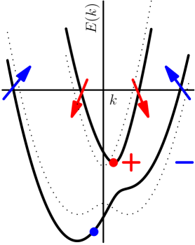
Figure 4: Occupied subbands $\epsilon_{\pm}$ for the case of non-orthogonal spin-orbital and magnetic field axes. Arrows illustrate spin polarization, as in Fig. 1. Filled dots indicate location of the center-of-mass for $(+)$ (red) and $(-)$ (blue) subbands. Dashed lines show $(\pm)$ subbands of Fig. 1, corresponding to the orthogonal orientation, $\beta=0$, for comparison.

The momentum-mismatch $\delta$ de-stabilizes the Cooper order and eventually, for some critical $\beta_{c}$, destroys it completely. The critical angle can be easily estimated by comparing two spatial scales: $\xi_{C}$, which describes perfect SDW order, and $1/\delta$, which represents the scale on which momentum-nonconservation becomes pronounced. Estimating $\xi_{C}\sim e^{\ell_{c}}$, where $\tilde{g}_{R}(\ell_{c})\sim 1$, we obtain that the Cooper order is destroyed when

$$U(2k_{F})(\alpha_{R}k_{F}\cos[\beta]/\Delta_{z})^{2}\approx\alpha_{R}k_{F}\sin[\beta].$$ (95)

Observe that this happens already for small angles, we can simplify the expression for the critical angle

$$\beta_{c}\propto\frac{U(2k_{F})}{\Delta_{z}}\frac{\alpha_{R}k_{F}}{\Delta_{z}}\ll 1.$$ (96)

This angular sensitivity of the found Cooper order to mutual orientation of the magnetic and spin-orbital directions can be used as an experimental probe to differentiate between it and other, spin-orbit independent, many-body instabilities of interacting quantum wire.

V Isolated Impurity

SDW_x state manifests itself not only in spin correlations (67). It turns out that its response to a weak potential scattering (impurity) is rather non-trivial. We consider here a weak delta-function impurity $V(x)=V_{0}\delta(x)$, with strength $V_{0}$, located at the origin. The condition $V_{0}\ll\Delta_{c}$ means that impurity can be considered as a weak perturbation to the established SDW phase. Since the latter is most robust in the limit of $\gamma_{F}\ll 1$, this is the limit we consider in this Section. (The limit of strong impurity, $V_{0}\gg\Delta_{c}$, is rather standard: impurity destroys the SDW and the wire flows into an insulator at low energies kane-fisher .)

The interaction of electrons with an impurity potential $V(x)$ is given by

$$\hat{V} = \int dx~{}V(x)\sum_{s=\uparrow,\downarrow}\Psi^{\dagger}_{s}(x)\Psi_{s}(x).$$ (97)

As usual, it is the backscattering ($\rho_{2k_{F}}$) part of the density that has to be considered, $\rho_{2k_{F}}=\sum_{s}(R^{\dagger}_{s}L_{s}+\text{h.c.})$. Working in the two-subband basis of eigenstates $\nu=\pm$ of the non-interacting Hamiltonian which includes Rashba spin-orbit term and the Zeeman term, see (18), we derive for the $2k_{F}$-component of the density $\rho(x)$ at the origin

$$\rho_{2k_{F}}=\rho_{2k_{F}}^{\text{intra}}+\rho_{2k_{F}}^{\text{inter}},$$ (98)

where the intra-subband part is

$$\rho_{2k_{F}}^{\text{intra}}=\cos[\gamma_{F}](L^{\dagger}_{+}R_{+}+L^{\dagger}_{-}R_{-}+\text{h.c.}),$$ (99)

while the novel inter-subband contribution is present due to the non-orhogonality of spin states in $(\pm)$ subbands discussed in Section II,

$$\rho_{2k_{F}}^{\text{inter}}=\sin[\gamma_{F}](L^{\dagger}_{-}R_{+}-L^{\dagger}_{+}R_{-}+\text{h.c.}).$$ (100)

Alternatively, one can think of these two contributions as representing $\tilde{\rho}$ and $\tilde{h}^{y}$ contributions in (75). In terms of bosonic fields the density reads

$$\rho_{2k_{F}}(x=0) = \frac{-2\sin[\sqrt{2\pi}\varphi_{\rho}]}{\pi a_{0}}\Big{(}\cos[\gamma_{F}]\cos[\sqrt{2\pi}\varphi_{\sigma}]$$ (101)

$$-\sin[\gamma_{F}]\cos[\sqrt{2\pi}\theta_{\sigma}]\Big{)}.$$

We now observe that setting $\theta_{\sigma}\to\theta_{\sigma}^{\text{cl}}=(m+\frac{1}{2})\sqrt{\pi/2}$, as appropriate for the Cooper phase (Section III.3), nullifies the backscattering component of the density (101). The first (intra-subband) term gets killed by diverging fluctuations of $\varphi_{\sigma}$, dual to $\theta_{\sigma}$. Intriguingly, the second (inter-subband) contribution is also zero because $\cos[\sqrt{2\pi}\theta_{\sigma}^{\text{cl}}]=\pm\cos[\pi/2]=0$.

This argument can be made more precise by following calculations described in Refs. review, ; orignac, ; egger, . We parametrize $\theta_{\sigma}=\theta_{\sigma}^{\text{cl}}+\delta\theta$ and expand the relevant cosine term in Hamiltonian (41) to second order in fluctuations $\delta\theta$. One obtains a massive term $\propto\Delta_{c}(\delta\theta)^{2}$ in the Hamiltonian, which causes exponential decay in correlation functions of the dual $\varphi_{\sigma}$ field. In particular $\langle\cos\sqrt{2\pi}\varphi_{\sigma}(0,\tau)\cos\sqrt{2\pi}\varphi_{\sigma}(0,\tau^{\prime})\rangle$ will decay as $\exp[-\Delta_{c}|\tau-\tau^{\prime}|]$. Thus for an incoming particle with energy $\omega\ll\Delta_{c}$, the inter-subband scattering channel is absent.

Substituting $\theta_{\sigma}=\theta_{\sigma}^{\text{cl}}+\delta\theta$ in the second term in (101) converts it into $\gamma_{F}\sin[\sqrt{2\pi}\varphi_{\rho}]\sin[\sqrt{2\pi}\delta\theta]$. Correlations of $\sin[\sqrt{2\pi}\delta\theta]$ are also short-ranged

$$\langle\sin[\sqrt{2\pi}\delta\theta(\tau)]\sin[\sqrt{2\pi}\delta\theta(\tau^{\prime})]\rangle\approx\frac{\Delta_{c}}{v_{F}k_{F}}\times$$

$$\sinh[K_{0}(\Delta_{c}|\tau-\tau^{\prime}|)],$$ (102)

where $K_{0}(x)\sim e^{-x}/\sqrt{x}$ (for $x\gg 1$) is the modified Bessel function (see Ref.review, ). The two exponentially decaying contibutions add up (in second order perturbation theory in impurity strength $V_{0}$) to produce an effective two-particle backscattering potential $\propto(V_{0}^{2}/\Delta_{c})\cos[\sqrt{8\pi}\varphi_{\rho}(0,\tau)]$. This generated two-particle impurity backscattering term, however, is relevant only for strongly repulsive interactions, $K_{\rho}<1/2$. We are thus left with irrelevant impurity potential for as long as $V_{0}\ll\Delta_{c}$ is justified and for not too strong repulsion, $1/2\leq K_{\rho}\leq 1$: SDW_x state is not sensitive to weak disorder!

The situation is similar to that in recently proposed edge states in quantum spin Hall system kane05 . There, gapless spin-up and spin-down excitations propagate in opposite directions along the edge, which forbids single-particle backscattering. Interacting electrons, however, can backscatter off the impurity in pairs xu06 ; wu06 .

Our conclusion $\rho_{2k_{F}}\to 0$, eq.(101), rests on somewhat technical condition $\cos[\sqrt{2\pi}\theta_{\sigma}^{\text{cl}}]=0$ and deserves a better understanding. This is provided by the perturbative calculation in Appendix D. The idea of the calculation is similar to that in Section IV: treat both impurity and spin-orbit terms as perturbation and generate spin-orbit-related corrections to backscattering potential (proportional to $\gamma_{F}$ in (101)) perturbatively. In this way we can be certain that all symmetry-allowed contributions are accounted for. This argument also makes it clear that the generated terms, being produced by the SOI, have to be odd under spatial inversion ${\cal P}$. It is this symmetry that guaranties that $\sin[\sqrt{2\pi}\theta_{\sigma}]$ can not be generated in the process. This instructive calculation, carried in Appendix D, indeed supports the conclusions of the more formal two-subband approach described in this Section.

We conclude this Section by pointing out experimental consequences of our findings. Suppression of single-particle backscattering off weak impurity under the outlined conditions implies an unusual negative magnetoresistance in one-dimensional wire. Indeed, the conductance of the wire with such an impurity should remain at the perfect $G_{\rm wire}=2e^{2}/h$ value for as long as applied magnetic field is directed perpendicular to the spin-orbital ($\sigma^{x}$ here) axis. By either turning the magnetic field off, or simply rotating the sample (so that momentum mismatch between the two subbands destabilizes SDW_x order), one should observe that conductance plateau deteriorates. It will be destroyed completely in the zero-temperature limit.

VI Heisenberg antiferromagnet with DM interaction and magnetic field

In this section we will consider a closely related problem: the effect of uniform and staggered Dzyaloshisnkii-Moriya (DM) interaction on a spin $S=1/2$ Heisenberg antiferromagnet (HAFM) in the presence of a magnetic field perpendicular to the DM vector. We start by demonstrating the equivalence between the quantum wire problem, analyzed in the previous Sections, with that of Heisenberg spin chain subject to an additional uniform DM interaction. We then present a novel chiral rotation argument to show that results of the two-subband approach in Section III can be obtained from a straightforward combination of two independent rotations for right- and left-movers. We also discuss the difference between the uniform and the staggered DM interaction, analyzed previously in Ref. ao, .

VI.1 Weak uniform DM interaction and strong Magnetic Field

The Hamiltonian of an isotropic HAFM spin chain is given by

$$H_{\text{heis}}=J\sum_{j}[S^{x}_{j}S^{x}_{j+1}+S^{y}_{j}S^{y}_{j+1}+S^{z}_{j}S^{z}_{j+1}].$$ (103)

In the continuum limit, the above Hamiltonian is most conveniently described in terms of the SU$(2)_{1}$ Wess-Zumino-Novikov-Witten model the basic ingredients of which are the uniform $SU(2)$ left $\vec{J}_{L}(x)$ and right $\vec{J}_{R}(x)$ spin currents, defined via fermions in (86), and the staggered magnetization $\vec{N}(x)$ gnt-book . Another important component is provided by staggered energy density (dimerization), see eq.(69), but this does not develop any order in the presence of external magnetic field. These operators will be used to represent the continuum limit of the spin,

$$\vec{S}_{j}\rightarrow a_{0}\Big{(}\vec{J}_{L}(x)+\vec{J}_{R}(x)+(-1)^{x/a_{0}}\vec{N}(x)\Big{)},$$ (104)

where $a_{0}$ is the lattice spacing and continuous space variable is introduced via $x=ja_{0}$. Continuum limit of (103) is $H_{\text{heis}}=H_{0}+H_{\text{bs}}$, where

$$H_{0} = \frac{2\pi v}{3}\int dx~{}\vec{J}_{R}\cdot\vec{J}_{R}+\vec{J}_{L}\cdot\vec{J}_{L}$$ (106)

$$=\frac{v}{2}\int dx~{}(\partial_{x}\varphi)^{2}+(\partial_{x}\theta)^{2}.$$

The first line constitutes nonabelian spin current formulation of the problem, which is convenient for analyzing spin-rotation invariant (SU(2)) problems, while the second makes connection with familiar abelian bosonization result (40): identifications $(\varphi_{\sigma},\theta_{\sigma})\to(\varphi,\theta)$, $u_{\sigma}\to v=\pi Ja_{0}/2$ and $k_{F}\to\pi/(2a_{0})$ finalize the connection. The marginal backscattering term accounts for residual interaction between spin excitations,

$$H_{\text{bs}}=-g_{\text{bs}}\int dx\vec{J}_{R}\cdot\vec{J}_{L}.$$ (107)

Its coupling constant $g_{\text{bs}}>0$ is known from extensive numerical studies of the Heisenberg chain eggert96 : $g_{\text{bs}}=0.23\times 2\pi v$. This term is responsible for the fact that initial value of the Luttinger parameter $K_{\sigma}=1+g_{\text{bs}}/2\pi v$ is greater than $1$.

There are no low energy charge fluctuations as the charge is “locked” to the lattice by relevant Umklapp processes. This allows one to replace cosine of charged boson $\varphi_{\rho}$ in (67) by its expectation value $\lambda$: $\lambda=\langle\cos[\sqrt{2\pi}\varphi_{\rho}]\rangle$. The first line of (67) then establishes abelian representation of the staggered magnetization

$$\left(\begin{array}[]{c}N^{x}\\ N^{y}\\ N^{z}\end{array}\right)=\frac{\lambda(-1)^{x}}{\pi a_{0}}\left(\begin{array}[]{c}-\sin[\sqrt{2\pi}\theta]\\ \cos[\sqrt{2\pi}\theta]\\ -\sin[\sqrt{2\pi}\varphi]\end{array}\right).$$ (114)

Magnetic field is introduced via Zeeman term

$$H_{Z}^{(z)}=-\sum_{j}g\mu_{B}BS^{z}_{j}\to-\Delta_{z}\int dx(J^{z}_{R}+J^{z}_{L}),$$ (115)

which is identical to (84). The small upper index ($z$ here) indicates the axis in spin space. Finally, the Dzyaloshinskii-Moriya Hamiltonian describes asymmetric and odd under spatial inversion interaction between spins

$$H_{\text{DM}}^{(x)}=\sum_{j}\vec{D}\cdot\vec{S}_{j}\times\vec{S}_{j+1}.$$ (116)

Vector $\vec{D}=D\hat{x}$ fixes direction of spin anisotropy, which we choose to be along spin-$\hat{x}$ direction, similar to the spin-orbit direction choice in (3).

Using (104) we see that continuum limit of the uniform DM Hamiltonian requires the knowledge of the following operators

$$O_{J}(x,x^{\prime}) = J^{y}(x)J^{z}(x^{\prime})-J^{z}(x)J^{y}(x^{\prime}),$$

$$O_{N}(x,x^{\prime}) = N^{y}(x)N^{z}(x^{\prime})-N^{z}(x)N^{y}(x^{\prime}),$$ (117)

where $x^{\prime}=x+a_{0}$. The first of these follows from the well-known OPE for spin currents, see for example eq.(25,26) of Ref. sfb, and set $\bar{z}-\bar{z}^{\prime}=ia_{0}$:

$$O_{J}(x,x^{\prime})=\frac{1}{\pi a_{0}}(J^{x}_{R}(x)-J^{x}_{L}(x)).$$ (118)

The second requires more work and is calculated using the definition (114) and bosonic OPEs (165)

$$O_{N}(x,x^{\prime})=\frac{2\lambda^{2}}{\pi a_{0}}(J^{x}_{R}(x)-J^{x}_{L}(x)).$$ (119)

As a result

$$H_{\text{DM}}^{(x)}=\tilde{D}\int dx~{}(J^{x}_{R}-J^{x}_{L})~{},~{}\tilde{D}=\frac{Da_{0}}{\pi}(1+2\lambda^{2}).$$ (120)

Comparing (120) with (85) and (115) with (84) we observe that the problem at hand is identical to that analyzed in Section IV. We immediately conclude that the $2k_{F}=\pi$ (staggered) components of spins acquire long range order along the direction of $\vec{D}$ as soon as magnetic field is turned on along the orthogonal direction.

$$\langle N^{x}\rangle={\text{const}}~{}(-1)^{x},~{}\langle N^{y,z}\rangle=0.$$ (121)

It is useful to compare this equation with (67). Note that the effect is controlled by the backscattering amplitude $g_{\text{bs}}=2(K_{\sigma}-1)$.

Except for the brief remark in section VIII of Ref.bocquet, , the possibility of the long-range order in the magnetized spin chain with asymmetric uniform DM interaction has not been discussed in the literature, to the best of our knowledge. We also would like to note technical similarities of our problem with that of an anisotropic Heisenberg chain in a transverse field, considered in Ref.caux03, .

Experimentally, the field-induced long-ranged magnetic order would be probably easiest to observe via thermodynamic measurements. Similar to the case of copper benzoate dender97 , the order should show up via an exponential suppression of the specific heat. The magnitude of this suppression, which is controlled by the energy gap $\Delta_{c}$ (55), should be a sensitive function of the magnetic field orientation, reaching maximum when the field is orthogonal to the DM axis as discussed above.

VI.2 Chiral rotation and tilted magnetic field

We now present an elegant argument, borrowed from the technically closely related study of quantum kagomé antiferromagnet kagome , exposing the nature of the Cooper order to the fullest. Consider the situation, discussed in Section IV.1, of the tilted magnetic field making an angle $\pi/2-\beta$ with the DM axis direction (which we keep at $\hat{x}$). The Hamiltonian describing this arrangement is given by $H=H_{0}+H_{\text{bs}}+V$, where $V$ includes Zeeman and DM fields

$$V=\int dx\Big{(}d_{R}J^{x}_{R}-d_{L}J^{x}_{L}-h_{1}(J^{z}_{R}+J^{z}_{L})\Big{)}.$$ (122)

The parameters are

$$d_{R}=\tilde{D}-h_{2},~{}d_{L}=\tilde{D}+h_{2},~{}h_{1}=h\cos\beta,~{}h_{2}=h\sin\beta.$$ (123)

We now rotate right (left) spin currents $\vec{J}_{R}$ ($\vec{J}_{L}$) about $\hat{y}$ axis by angle $\theta_{R}$ ($\theta_{L}$) such that after the rotation the $V$-term becomes

$$V=-\int dx\Big{(}\sqrt{d_{R}^{2}+h_{1}^{2}}~{}M^{z}_{R}+\sqrt{d_{L}^{2}+h_{1}^{2}}~{}M^{z}_{L}\Big{)}.$$ (124)

The relation between old ($\vec{J}$) and new ($\vec{M}$) currents is simple

$$\vec{J}_{R}={\cal R}(\theta_{R})\vec{M}_{R},~{}~{}~{}\vec{J}_{L}={\cal R}(\theta_{L})\vec{M}_{L},$$ (125)

here ${\cal R}$ is the rotation matrix

$${\cal R}(\theta)=\left(\begin{array}[]{ccc}\cos[\theta]&0&-\sin[\theta]\\ 0&1&0\\ \sin[\theta]&0&\cos[\theta]\\ \end{array}\right).$$ (129)

The rotation angles are given by $\tan[\theta_{R}]=d_{R}/h_{1}$ and $\tan[\theta_{L}]=-d_{L}/h_{1}$. The key reason behind these rotations is the observation that unperturbed Hamiltonian $H_{0}$, being the sum of commuting right and left terms, is invariant under the rotations. But the backscattering $H_{\text{bs}}$ is not, and transforms into

$$H_{\text{bs}} = -g_{\text{bs}}\int dx\Big{(}\cos[\gamma](M^{x}_{R}M^{x}_{L}+M^{z}_{R}M^{z}_{L})$$ (130)

$$+\sin[\gamma](M^{x}_{R}M^{z}_{L}-M^{z}_{R}M^{x}_{L})+M^{y}_{R}M^{y}_{L}\Big{)},$$

where $\gamma=\theta_{R}-\theta_{L}$. The reason for this transformation is of course that right and left currents are rotated in opposite directions (and by different amounts). Observe that (130) matches the interaction part of (51).

The nice thing about the rotation is that now both SO and Zeeman fields can be taken into account by simple linear transformations of spin bosons. Indeed, using abelian bosonization we observe that

$$V=-\int dx\Big{(}\frac{vt_{\varphi}}{\sqrt{2\pi}}\partial_{x}\varphi_{\sigma}+\frac{vt_{\theta}}{\sqrt{2\pi}}\partial_{x}\theta_{\sigma}\Big{)},$$ (131)

where

$$t_{\varphi}=(\sqrt{d_{L}^{2}+h_{1}^{2}}+\sqrt{d_{R}^{2}+h_{1}^{2}})/2v,$$

$$t_{\theta}=(\sqrt{d_{L}^{2}+h_{1}^{2}}-\sqrt{d_{R}^{2}+h_{1}^{2}})/2v.$$ (132)

These linear terms are removed by shifts

$$\varphi_{\sigma}\to\varphi_{\sigma}+\frac{t_{\varphi}x}{\sqrt{2\pi}},$$

$$\theta_{\sigma}\to\theta_{\sigma}+\frac{t_{\theta}x}{\sqrt{2\pi}}.$$ (133)

The price is that transverse components $M^{x,y}_{R/L}$ acquire oscillating position-dependent factors

$$M^{+}_{R}\to M^{+}_{R}e^{-i(t_{\varphi}-t_{\theta})x},~{}~{}~{}M^{+}_{L}\to M^{+}_{L}e^{i(t_{\varphi}+t_{\theta})x}.$$ (134)

The major consequence of this is that every term in $H_{\text{bs}}$, with a single exception of $M^{z}_{R}M^{z}_{L}$ one, picks up oscillating factor

$$H_{\text{bs}}=-g_{\text{bs}}\int dx\Big{(}\cos[\gamma]M^{z}_{R}M^{z}_{L}+$$

$$+\frac{\cos[\gamma]-1}{4}(M^{+}_{R}M^{+}_{L}e^{i2t_{\theta}x}+{\text{h.c.}})$$

$$+\frac{\cos[\gamma]+1}{4}(M^{+}_{R}M^{-}_{L}e^{-i2t_{\varphi}x}+{\text{h.c.}})$$ (135)

$$+\frac{\sin[\gamma]}{2}(M^{z}_{L}M^{+}_{R}e^{-i(t_{\varphi}-t_{\theta})x}-M^{z}_{R}M^{+}_{L}e^{i(t_{\varphi}+t_{\theta})x}+{\text{h.c.}})\Big{)}.$$

This equation contains all arrangements that we have discussed in this paper. Setting $t_{\theta}=0$ corresponds to orthogonal ($\beta=0$) orientation of spin-orbit (DM) and magnetic field axis. In that limit we recover equations (49) ($\vec{J}$ there corresponds to $\vec{M}$ here). Allowing for $\beta>0$ leads us to Section IV.1, results of which represent abelian version of the discussion here. As shown there, the SDW_x phase is stable in a finite angular interval near $\beta=0$.

It is worth noting that (124) and (131) imply finite expectation values of $M^{z}_{R/L}$ currents:

$$\langle M^{z}_{R/L}\rangle=\sqrt{d_{R/L}^{2}+h_{1}^{2}}/(4\pi v).$$ (136)

By virtue of (129) this implies finite expectation values of the uniform magnetization along $z$ and $x$ axis, $J^{z/x}_{R}+J^{z/x}_{L}$, and uniform spin current, $J^{z/x}_{R}-J^{z/x}_{L}$, along these two axes. That is,

$$\langle J^{x}_{R}-J^{x}_{L}\rangle=\sin[\gamma]\frac{t_{\phi}}{2\pi},\langle J^{z}_{R}-J^{z}_{L}\rangle=-\cos[\gamma]\frac{t_{\theta}}{2\pi},$$

$$\langle J^{x}_{R}+J^{x}_{L}\rangle=-\sin[\gamma]\frac{t_{\theta}}{2\pi},\langle J^{z}_{R}+J^{z}_{L}\rangle=\cos[\gamma]\frac{t_{\phi}}{2\pi}.$$ (137)

Equilibrium values of spin current and magnetization along the $y-$direction vanish. These relations complement discussion of the relations between staggered ($2k_{F}$) components of various fields in Section III.3.

VI.3 Strong uniform DM interaction and weak Magnetic Field

It is instructive to consider another ‘tricky’ limit of the problem: strong uniform DM interaction and a weak magnetic field, $D\gg\Delta_{z}$. The idea here is to account for the DM term exactly on the lattice level, see (138), and treat the Zeeman term as a small perturbation to the obtained Hamiltonian (140).

The two axis, DM and Zeeman, are still orthogonal but it is more convenient now to let $\vec{D}$ point along the $\hat{z}$-axis in spin space, while magnetic field is pointing along $\hat{x}$. Following Ref. bocquet, we perform unitary transformation of the lattice Hamiltonian to absorb the uniform DM term exactly,

$$S_{j}^{+}\rightarrow\tilde{S}_{j}^{+}e^{i\alpha j}~{},~{}S_{j}^{-}\rightarrow\tilde{S}_{j}^{-}e^{-i\alpha j}~{}\text{and}~{}S^{z}_{j}\rightarrow\tilde{S}^{z}_{j},$$ (138)

where $\alpha=\arctan(D/J)\approx D/J$ for $D\ll J$. The transformed Hamiltonian is that of the XXZ spin chain with weak anisotropy

$$\tilde{H}=\tilde{J}\sum_{j}[\tilde{S}^{x}_{j}\tilde{S}^{x}_{j+1}+\tilde{S}^{y}_{j}\tilde{S}^{y}_{j+1}+\frac{J}{\tilde{J}}\tilde{S}^{z}_{j}\tilde{S}^{z}_{j+1}],$$ (139)

where $\tilde{J}=\sqrt{J^{2}+D^{2}}$. Magnetic field term, however, acquires position dependence under this transformation

$$\tilde{H}_{Z}^{(x)}=-\frac{\Delta_{z}}{2}\sum_{j}(\tilde{S}^{+}_{j}e^{i\alpha j}+\tilde{S}^{-}_{j}e^{-i\alpha j}).$$ (140)

Bosonizing it according to the rules described in Sec. III.1 and IV, we obtain

$$\tilde{H}_{Z}^{(x)}=\frac{\eta_{\uparrow}\eta_{\downarrow}\Delta_{z}}{\pi a_{0}}\int dx\sin[\sqrt{2\pi K}\varphi]\cos[\sqrt{\frac{2\pi}{K}}\theta+\alpha x],$$ (141)

where Luttinger parameter of the XXZ chain (139) is given by $K^{-1}=1-\arccos[J/\sqrt{J^{2}+D^{2}}]/\pi\approx 1-D/(\pi J)$. The shift of $\theta$ field by $\alpha x$ can be easily understood from equation (120), adapted for the DM axis along $\hat{z}$-direction in spin space: $H_{\text{DM}}^{(z)}=\tilde{D}\int dx(J^{z}_{R}-J^{z}_{L})\propto\tilde{D}\int dx~{}\partial_{x}\theta$ which indeed can be accounted for by shifting $\theta$.

Being of nonzero conformal spin, the Zeeman term (141) generates under RG two new terms of importance to us: $\tilde{H}_{\varphi}\propto(\Delta_{z}^{2}D/J)\cos[\sqrt{8\pi K}\varphi]$, of scaling dimension $2K=2+2D/(\pi J)>2$, and $\tilde{H}_{\theta}=G_{\theta}\int dx\cos[\sqrt{\frac{8\pi}{K}}\theta+2\alpha x]$ with scaling dimension $2/K=2-2D/(\pi J)<2$. The position-dependent phase $2\alpha x$, nonetheless, makes it irrelevant.

Indeed, the coupling constant can be estimated, following momentum-shell RG of Appendix C, as $G_{\theta}\propto(\Delta_{z}/v)^{2}(K-1/K)^{2}\approx(\Delta_{z}D/J)^{2}$, see (183) and (190). Neglecting the oscillating phase for the moment, we can easily estimate the correlation length corresponding to the Cooper order as $\xi_{c}=\exp[\ell_{c}]$, where $G_{\theta}(\ell_{c})=G_{\theta}(0)\exp[(2-2/K)\ell_{c}]\approx 1$, so that $\ell_{c}=(\pi J/D)\ln[J/(\Delta_{z}D)]$.

This length is to be compared with $\xi_{\alpha}=1/\alpha\approx J/D$, which is the length on which the cosine in $\tilde{H}_{\theta}$ changes sign. We observe that

$$\ln[\xi_{c}]=\frac{\pi J}{D}\ln\Big{(}\frac{J}{\Delta_{z}D}\Big{)}\gg\ln[\xi_{\alpha}]=\ln(\frac{J}{D})$$ (142)

which implies that fast oscillations make it impossible for the $\tilde{H}_{\theta}$ to reach strong coupling. Hence no order can come from this term.

The other term, $\tilde{H}_{\varphi}$, appears to be irrelevant and it is tempting to disregard it altogether. One however must be careful and recall discussion in Section III.2. Particularly, observe that $\tilde{H}_{\varphi}$ may fall in region II (with $y_{\sigma}(0)<0$). Whether or not this happens is in principle a subject of precise calculation which however can be avoided here. Indeed analysis of Section VI.2, taken together with results of Sec. III.2, shows that Cooper instability develops for arbitrary $\gamma$ as long as $t_{\theta}=0$.

We thus conclude that $\tilde{H}_{\varphi}$ must belong to region II in Figure 3, even though this conclusion is not at all obvious from the abelian bosonization analysis sketched above. We chose to present this subtle point in order to demonstrate the power of non-abelian current formulation in Section VI.2.

Note finally that $\tilde{H}_{\varphi}$ still describes Cooper order even though it is written in terms of $\varphi$ field. The reason for this illustrates another shortcoming of abelian formulation. Unitary transformation (138) is the lattice version of rotation of right (left) currents by $\theta_{R}=\pi/2$ ($\theta_{L}=-\pi/2$) in the previous Section. (In this limit $\Delta_{z}=0$ and magnetic field is to be added later as a perturbation.) Such a rotation corresponds to $\gamma=\pi$ which replaces standard backscattering $(M^{+}_{R}M^{-}_{L}+{\text{h.c.}})$ with $(M^{+}_{R}M^{+}_{L}+{\text{h.c.}})$. In terms of abelian bosonization this corresponds to interchange $\cos\sqrt{8\pi}\varphi\leftrightarrow\cos\sqrt{8\pi}\theta$. Moreover, this same notation changes the sign of $M^{z}_{R}M^{z}_{L}$ term, which corresponds to interchange $K\leftrightarrow 1/K$, which completes the duality mapping. Observe again the ease with which current formulation of Section VI.2 leads to conclusion.

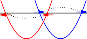
Figure 5: Band structure in the absence of magnetic field. Note the absence of the gap between the subbands at $k=0$.

In simpler terms, accounting for DM (or, equivalently, spin-orbit) term only amounts to working in the basis of eigenstates of operator $\sigma_{x}$. These eigenstates are described simply by two horizontally shifted parabolas in Figure 5. Denoting the right (left) subbands by index $1$ ($|1\rangle=|\rightarrow\rangle$) and $2$ ($|2\rangle=|\leftarrow\rangle$) we immediately observe that Cooper scattering discussed previously corresponds to the process like $R^{\dagger}_{1}L_{1}L^{\dagger}_{2}R_{2}$. (So that initial pair $L_{1}R_{2}$ scatters to final $R_{1}L_{2}$ state. Note that the other possibility, $L_{1}\to L_{2}$ and $R_{2}\to R_{1}$ is forbidden by orthogonality of single-particle basis states, $\langle 1|2\rangle=\langle\rightarrow|\leftarrow\rangle=0$.) Bosonizing this in a standard way we find that (recall $R^{\dagger}_{1}L_{1}\sim\exp[-i\sqrt{4\pi}(\phi_{1R}+\phi_{1L})]$) $R^{\dagger}_{1}L_{1}L^{\dagger}_{2}R_{2}\sim\exp[-i\sqrt{4\pi}(\varphi_{1}-\varphi_{2})]=\exp[-i\sqrt{8\pi}\varphi_{\sigma}]$. Thus indeed the Cooper process is written in terms of $\varphi_{\sigma}$ field in the new basis.

Observe that this conclusion is special to the limit of no magnetic field, $\Delta_{z}=0$. As soon as the field is on, $\Delta_{z}\neq 0$, the band structure changes and horizontally shifted subbands $(1,2)$ turn into vertically shifted pair $(-,+)$ used in this paper (Fig. 1): arbitrary small $B$ leads to the gap $\Delta_{z}$ at the point $k=0$, see (4). We thus conclude once again that $\Delta_{z}=0$ is a rather singular limit, not much suited for the consideration of general situation with both spin-orbit and Zeeman fields present.

VI.4 HAFM chain with staggered DM interaction and magnetic field

For the sake of completeness and uniformity of the presentation, we re-visit here the well-studied case of interplay between staggered DM interaction and Zeeman magnetic field, described in Refs. ao, and oshikawaJPSJ, .

Staggered DM interaction along $\hat{x}$-axis is described by

$$H_{\text{sDM}}^{(x)}=D\sum_{j}(-1)^{j}(S^{y}_{j}S^{z}_{j+1}-S^{z}_{j}S^{y}_{j+1}).$$ (143)

Its continuum limit requires the knowledge of

$$O_{JN}(x,x^{\prime}) = N^{y}(x)J^{z}(x^{\prime})+J^{z}(x)N^{y}(x^{\prime})$$ (144)

$$-J^{y}(x)N^{z}(x^{\prime})-N^{z}(x)J^{y}(x^{\prime}),$$

where, as before in (117), we set $x^{\prime}=x+a_{0}$. It is an easy calculation, using eq.26 of Ref.sfb, , to find that in the absence of magnetic field $O_{JN}=0$ identically. The situation changes when magnetic field (along $\hat{z}$-axis) is present. Using bosonization, magnetic field is accounted for (see (IV) and line above it) by the shift $\sqrt{2\pi K}\varphi\to\sqrt{2\pi K}\varphi+q_{0}x$. Moreover, the main effect of the field here is contained in $q_{0}=\Delta_{z}/v$ and we can keep $K=1$ in all calculations below. Observing that a shift in $\varphi$ implies equal shifts in $\phi_{R/L}$ fields (so that $\theta$ does not change) and working backward through (67), (86) and (26) we conclude, following Ref.ao, , that in the presence of the magnetic field, spin excitations along the field ($\hat{z}$-axis here) and transverse to it ($\hat{x},\hat{y}$ axis) have minima at different momenta. Namely, while $J^{z}$ is still centered at $q=0$, transverse components of spin current $J^{x,y}$ acquire minima at $q=\pm q_{0}=\pm 2\pi m$, where $m$ is the magnetization. In addition, $N^{z}$ shifts from $\pi$ to $q=\pi\pm 2\pi m$ while staggered transverse components $N^{x,y}$ remain at $2k_{F}=\pi$ point. As a result, the product $N^{y}J^{z}$ (first line in (144)) retains its zero-field structure and continues to remain at zero. At the same time the other combination, $J^{y}N^{z}$ (second line in (144)), splits into slow ($e^{iq_{0}(x-x^{\prime})}$) and fast ($e^{iq_{0}(x+x^{\prime})}$) oscillating pieces which do not cancel each other anymore. The remaining calculation is most conveniently performed using fermionic representations of spin currents (86) and longitudinal magnetization $N^{z}=\frac{1}{2}[R^{\dagger}_{\uparrow}L_{\uparrow}-L^{\dagger}_{\downarrow}R_{\downarrow}]e^{-iq_{0}x}+\text{h.c.}$. Fusing right (left) movers of like spin using (200) we obtain, for example,

$$(J^{+}_{R}(x)+J^{+}_{L}(x))N^{z}(x^{\prime})=-\frac{\sin[q_{0}(x-x^{\prime})]}{2\pi(x-x^{\prime})}(R^{\dagger}_{\uparrow}L_{\downarrow}+L^{\dagger}_{\uparrow}R_{\downarrow}).$$ (145)

Bosonizing this expression (note that it is not sensitive to the sign of the coordinate difference $(x-x^{\prime})$) we finally obtain

$$O_{JN}(x,x^{\prime})=-\frac{q_{0}\lambda}{2\pi^{2}a_{0}}\cos[\sqrt{2\pi}\theta(x)].$$ (146)

The same result can be obtained, after somewhat longer calculation, using bosonized forms of spin currents and magnetization from the very beginning. The continuum limit of staggered DM term then follows

$$H_{\text{sDM}}^{(x)}=\frac{Dq_{0}\lambda}{\pi^{2}a_{0}}\int dx~{}\cos[\sqrt{2\pi}\theta(x)].$$ (147)

This is a highly relevant operator (scaling dimension $1/2$), the coupling constant $G_{\text{s-dm}}$ of which grows as $G_{\text{s-dm}}(\ell)=G_{\text{s-dm}}(0)\exp[3\ell/2]$. This, and the dependence of its initial value on the combination $D\Delta_{z}$ (which enters via dependence on $q_{0}$), leads to the energy gap in the system that scales as $(D\Delta_{z})^{2/3}$, exactly as Ref.ao, found originally. Note finally that (147) and (67) implies that the spins order (in a staggered way) along $\hat{y}$-axis, orthogonal to both DM and magnetic field directions.

Note that although we have treated staggered DM term (143) as a perturbation to the spin chain subject to magnetic field (which comes in via the momentum $q_{0}$ here), we obtained the same strongly relevant result (147) as the authors of Ref. ao, did. But Ref. ao, arrived at it from a different limit: the authors used staggered version of (138) to account for DM piece (143) exactly and then added magnetic field as a perturbation. The outcome (147) is obtained in both cases simply because it is more relevant (dimension $1/2$) than the magnetic field (Zeeman) term (dimension $1$): no matter how small $G_{\text{s-dm}}$ initially is, it controls the physics. The $N^{y}$-order is present for any ratio of $G_{\text{s-dm}}/\Delta_{z}$ ratio.

VII Implications for ESR experiments

In recent years, electron spin resonance (ESR) technique has become a leading experimental candidate for probing anisotropic terms in the spin chain. Recent theoretical impetus to this field has been provided in an important work by Oshikawa and Affleck oa-esr ; oa who discussed limitations of earlier theoretical work kubo-tomita ; mori-kawasaki1 ; mori-kawasaki2 and improved and extended upon them by using powerful modern theoretical techniques. The emphasis in oa has been to study the role of anisotropic terms, in particular the staggered DM interaction, see Section VI.4, and exchange anisotropy terms, in modifying the resonance position and the line width. However, ESR in a spin chain with uniform DM interaction was not considered. We will follow a closely related work by De Martino et al. egger02 ; egger04 , who considered ESR for carbon nanotubes with spin-orbit coupling, to investigate the modifications brought upon by the uniform DM term on the ESR spectra.

We consider Faraday configuration in which the static magnetic field and oscillating field are orthogonal to each other. The oscillating driving field (of frequency $\omega$) is in the microwave frequency regime and for all practical purposes the spatial modulation of the field can be ignored. The ESR intensity is given by the transverse (to the static magnetic field) spin structure factor at $q=0$ and frequency $\omega$,

$$I(\omega)=\int dtdx~{}e^{i\omega t}\sum_{r,r^{\prime}=R/L}\langle J^{+}_{r}(x,t)J^{-}_{r^{\prime}}(0,0)\rangle.$$ (148)

As before, the Hamiltonian, $H=H_{0}+H_{bs}+V$, consists of the free part (106), the back scattering part (107), and the DM and Zeeman terms contained in the $V$ term (122). The angle between DM and magnetic field directions is $\pi/2-\beta$, see Section VI.2.

Our aim here is to present the basic picture of ESR response for the case of the spin chain with uniform DM interaction (equivalently, quantum wire with spin-orbit interaction). For this zeroth order description we omit the backscattering interaction (107) between the spin currents altogether. Under this drastic approximation right $\vec{J}_{R}$ and left $\vec{J}_{L}$ spin currents are decoupled. This implies the intensity (148) is the sum of right and left contributions, $I(\omega)=I_{R}(\omega)+I_{L}(\omega)$.

To account for the simultaneous presence of DM and Zeeman terms, we now rotate the right and left currents about the $y-$axis as described in Section VI.2, see in particular (125) and (129). As the backscattering (130) is neglected, the full Hamiltonian is given by

$$H = \int dx\sum_{a=x,y,z}\frac{2\pi v}{3}\Big{(}M^{a}_{R}M^{a}_{R}+M^{a}_{L}M^{a}_{L}\Big{)}$$ (149)

$$-\lambda_{R}M^{z}_{R}-\lambda_{L}M^{z}_{L},$$

where $\lambda_{R/L}=\sqrt{d_{R/L}^{2}+h_{1}^{2}}=v(t_{\varphi}\mp t_{\theta})$.

We now focus on the contribution of the right spin currents,

$$I_{R}(\omega)=\int dtdx~{}e^{i\omega t}\langle J^{+}_{R}(x,t)J^{-}_{R}(0,0)\rangle,$$ (150)

which, in terms of the rotated currents, reads

$$I_{R}(\omega) = \int dtdx~{}e^{i\omega t}\Big{(}\cos^{2}\theta_{R}\langle M^{x}_{R}(x,t)M^{x}_{R}(0)\rangle$$

$$+\langle M^{y}_{R}(x,t)M^{y}_{R}(0)\rangle+\sin^{2}\theta_{R}\langle M^{z}_{R}(x,t)M^{z}_{R}(0)\rangle\Big{)}.$$

The cross-terms of the kind $\langle M^{x}_{R}(x,t)M^{z}_{R}(0)\rangle=0$ due to the absence of coupling between $x$ and $z$ components in the Hamiltonian (149). Further, switching to $M^{\pm}_{R}$ combinations of the currents, the intensity becomes

$$I_{R}(\omega) = \int dtdx~{}e^{i\omega t}\Big{(}\sin^{2}\theta_{R}\langle M^{z}_{R}(x,t)M^{z}_{R}(0)\rangle$$

$$+\frac{(\cos^{2}\theta_{R}-1)}{4}\langle M^{+}_{R}(x,t)M^{+}_{R}(0)+\text{h.c.}\rangle$$

$$+\frac{(\cos^{2}\theta_{R}+1)}{4}\langle M^{+}_{R}(x,t)M^{-}_{R}(0)+\text{h.c.}\rangle\Big{)}.$$

The second line in this expression contributes zero as it requires anomalous averages of the kind $\langle\Psi_{R,\uparrow}(x,t)\Psi_{R,\uparrow}(0,0)\rangle$ which are absent in (149). We now absorb “right” magnetic field $\lambda_{R}$ via the shift of right boson so that $M^{+}_{R}\to M^{+}_{R}e^{-i\lambda_{R}x/v}$ (compare with (134)). It is worth noting that by rotating the spin currents we have mapped the problem of the spin chain with uniform DM and magnetic fields to that of the chain in field $\lambda_{R}$ ($\lambda_{L}$) for its right (left) moving components. This allows to borrow results of Ref. oa, and conclude that the first line in (VII) does not contribute to $I_{R}$ while the last line gives

$$I_{R}(\omega)=\frac{(\cos^{2}\theta_{R}+1)}{2}\omega\delta(\omega-|\lambda_{R}|).$$ (153)

Clearly the contribution of the left-moving sector is obtained by replacing $R\to L$ in the expression above. Thus the ESR signal consists of two sharp lines, as previously discussed for the case of carbon nanotube in Refs. egger02, ; egger04, ,

$$I(\omega) = (\cos^{2}\theta_{R}+1)\lambda_{R}\delta(\omega-|\lambda_{R}|)$$ (154)

$$+(\cos^{2}\theta_{L}+1)\lambda_{L}\delta(\omega-|\lambda_{L}|).$$

The distance between the lines is $\lambda_{L}-\lambda_{R}=2vt_{\theta}$. The relative strength of the two lines is

$$\frac{I_{R}(\lambda_{R})}{I_{L}(\lambda_{L})}=\sqrt{\frac{d_{L}^{2}+h_{1}^{2}}{d_{R}^{2}+h_{1}^{2}}}.$$ (155)

The ratio is always $1$ for $\beta=0$ (orthogonal orientation of DM and magnetic field axes), see (123). Note that this is exactly the configuration in which SDW order develops, as described in detail in Section III.2. The ordering is driven by the Cooper term, $H_{\sigma}^{C}$ in (49) (equivalently, the term proportional to $(\cos[\gamma]-1)$ in (VI.2)), which comes from the backscattering process as is made clear by the discussion in Section VI.2. The result (154), obtained by neglecting backscattering, is clearly not applicable at low temperature where the SDW (Cooper) instability develops. Well below the ordering temperature the system is described by the sine-Gordon model excitations of which are massive kinks zvyagin05 . But even above the ordering temperature in the disordered phase (which, for $\beta>0$ extends all way down to zero temperature, see Section IV.1) we expect the backscattering to affect the ESR signal. Whether or not it would lead to the finite linewidth of the two lines in (154) we do not understand yet and leave this interesting question (see Ref. oa, for detailed discussion of some technical subtleties) for future studies.

VIII Conclusions

Spin-orbital interactions result in reduction of spin-rotational symmetry from $SU(2)$ to $U(1)$ in one-dimensional quantum wires and spin chains. This reduction, however, is not sufficient to change the critical (Luttinger liquid) nature of the one-dimensional interacting fermions. The situation changes dramatically once external magnetic field is applied, as we have shown in this paper. Most interesting situation occurs when the applied field is oriented along the axis orthogonal to the spin-orbital (or, Dzyaloshinskii-Moriya, in case of spin chain) axis of the wire. The resulting combination of two non-commuting perturbations, taken together with electron-electron interactions, leads to a novel spin-density-wave order in the direction of the spin-orbital axis.

The physics of this order is elegantly described in terms of spin-non-conserving (Cooper) pair tunneling processes between Zeeman-split electron subbands. The tunneling matrix element is finite only due to the presence of the spin-orbit interaction, which allows for spin-up to spin-down (and vice versa) conversion.

The resulting SDW state affects both spin and charge properties of the wire. In particular, it suppresses effect of (weak) potential impurity, resulting in the interesting phenomena of negative magnetoresistance in one-dimensional setting, as described in Section V.

SDW ordering acquires true long-range nature in the case of spin chain, where charge fluctuations are absent. The staggered moment points along the DM axis and is orthogonal to the applied magnetic field.

Even when the magnetic field and spin-orbital directions are not orthogonal, an arrangement when the critical Luttinger state survives down to the lowest temperature (see Section IV.1), the problem remains interesting. In this geometry an ESR experiment should reveal two separate lines, which represent separate responses of right- and left-moving spin fluctuations in the system.

It is worth pointing out that unusual consequences of the interplay of spin-orbit and electron interactions are not restricted to one-dimensional systems only. We have recently shown vdW07 that Coulomb-coupled two-dimensional quantum dots acquire a novel van der Waals-like anisotropic interaction between spins of the localized electrons. The strength of this Ising interaction is determined by the forth power of the Rashba coupling $\alpha_{R}$.

We hope that our work will stimulate experimental search and studies of strongly interacting quasi-one-dimensional systems with sizable spin-orbital interaction, in particular regarding their response to the (both magnitude and direction) applied magnetic field and/or magnetization. ESR studies of spin chain materials with uniform DM interaction are very desirable as well.

We would like to thank I. Affleck, L. Balents, G. Fiete, C. Kane, D. Mattis, K. Matveev, E. Mishchenko, J. Moore, L. Levitov, J. Orenstein, M. Oshikawa, M. Raikh, K. Samokhin, and Y.-S. Wu for useful discussions and suggestions at various stages of this work. O.S. thanks the Petroleum Research Fund of the American Chemical Society for the financial support of this research under the grant PRF 43219-AC10.

Appendix A Derivation of intra-subband Hamiltonian (33)

Non-interacting (kinetic energy) part of the $\nu$-th subband ($\nu=\pm$) Hamiltonian reads

$$H^{0}_{\text{intra}}=\frac{v_{F}}{2}\int dx~{}(\partial_{x}\phi_{\nu})^{2}+(\partial_{x}\theta_{\nu})^{2}.$$ (156)

The intra-subband interaction term is given by the part of (16) which involves only densities from the $\nu$-th subband

$$H^{\prime}_{\text{intra}}=\frac{1}{2}\int dxdx^{\prime}U(x-x^{\prime})\rho_{\nu}(x)\rho_{\nu}(x^{\prime}),$$ (157)

where the density in the $\nu$-th subband is expressed with the help of (18) as

$$\rho_{\nu} = R^{\dagger}_{\nu}R_{\nu}+L^{\dagger}_{\nu}L_{\nu}+\cos[\gamma_{\nu}]$$ (158)

$$\times\Big{(}e^{-i2k_{\nu}x}R^{\dagger}_{\nu}L_{\nu}+e^{i2k_{\nu}x}L^{\dagger}_{\nu}R_{\nu}\Big{)}.$$

Its bosonized form follows

$$\rho_{\nu}=\frac{1}{\sqrt{\pi}}\partial_{x}\phi_{\nu}-\frac{\cos[\gamma_{\nu}]}{\pi a_{0}}\sin[\sqrt{4\pi}\phi_{\nu}+2k_{\nu}x],$$ (159)

where the first (second) term represents uniform ($2k_{\nu}$) parts of density. The interaction term (157) then naturally splits into a sum of two contributions

$$H^{\prime}_{\text{intra}}=H^{\prime}_{0}+H^{\prime}_{2k_{\nu}},$$

$$H^{\prime}_{0}=\frac{U(0)}{2\pi}\int dX~{}(\partial_{X}\phi_{\nu})^{2},$$ (160)

$$H^{\prime}_{2k_{\nu}}=\frac{\cos^{2}[\gamma_{\nu}]}{2(\pi a_{0})^{2}}\int dxdX~{}U(x)\sin[\sqrt{4\pi}\phi_{\nu}(X+x/2)+$$

$$+2k_{\nu}(X+x/2)]~{}\sin[\sqrt{4\pi}\phi_{\nu}(X-x/2)+$$

$$+2k_{\nu}(X-x/2)],$$ (161)

where $x\to x-x^{\prime}$ and $X=(x+x^{\prime})/2$ are the relative and center-of-mass coordinates, respectively.

Next, following Ref. giam00, , we fuse the two sines in (A) (the result is denoted as $S$ below) using (30) and OPE identities (165,166) to obtain

$$S(x,X) = \frac{a_{0}^{2}}{4x^{2}}\sum_{\mu=\pm}e^{i\mu 2k_{\nu}x}\times$$

$$\times\exp\{i\mu\sqrt{4\pi}[\phi(X+x/2)-\phi(X-x/2)]\}.$$

Performing gradient expansion in $x$, neglecting boundary contribution (equivalently, using periodic boundary conditions so that $\int dX~{}\partial_{X}\phi(X)=0$), and summing over $\mu=\pm 1$ leads to

$$H^{\prime}_{2k_{\nu}} = -\frac{\cos^{2}[\gamma_{\nu}]}{2\pi}\int dx~{}U(x)\cos[2k_{\nu}x]$$ (163)

$$\times\int dX~{}(\partial_{X}\phi_{\nu})^{2}.$$

The integral over relative distance gives backscattering component of the potential $U(2k_{\nu})$. Adding two contributions we find

$$H^{\prime}_{\text{intra}}=\frac{U(0)-\cos^{2}[\gamma_{\nu}]U(2k_{\nu})}{2\pi}\int dx~{}(\partial_{x}\phi_{\nu})^{2}.$$ (164)

The sum of (156) and (164) gives us the result (33).

Appendix B Perturbative Approach to Generate the Cooper term

Expansion (88) relies on the following operator product expansion (OPE)

$$:e^{i\alpha\phi_{R}(\bar{z})}::e^{i\beta\phi_{R}(\bar{z}^{\prime})}: = :e^{i[\alpha\phi_{R}(\bar{z})+\beta\phi_{R}(\bar{z}^{\prime})]}:$$

$$\times e^{-\alpha\beta\langle\phi_{R}(\bar{z})\phi_{R}(\bar{z}^{\prime})\rangle},$$

$$:e^{i\alpha\phi_{L}(z)}::e^{i\beta\phi_{L}(z^{\prime})}: = :e^{i[\alpha\phi_{L}(z)+\beta\phi_{L}(z^{\prime})]}:$$ (165)

$$\times e^{-\alpha\beta\langle\phi_{L}(z)\phi_{L}(z^{\prime})\rangle},$$

where $z=u_{\sigma}\tau+ix$ and $\bar{z}=u_{\sigma}\tau-ix$ and correlation functions of chiral bosons are defined by

$$\langle\phi_{L}(z)\phi_{L}(z^{\prime})\rangle = -\frac{1}{4\pi}\ln(\frac{z-z^{\prime}}{a_{0}}),$$

$$\langle\phi_{R}(\bar{z})\phi_{R}(\bar{z}^{\prime})\rangle = -\frac{1}{4\pi}\ln(\frac{\bar{z}-\bar{z}^{\prime}}{a_{0}}).$$ (166)

Both (165) and (166) follow from the harmonic $S_{0}$, see (89). We also employ Baker-Hausdorff formulae

$$e^{A}e^{B}=e^{B}e^{A}e^{[A,B]}~{},~{}e^{A}e^{B}=e^{A+B}e^{\frac{1}{2}[A,B]}$$ (167)

to convert expressions in terms of dual bosons $\varphi_{\sigma},\theta_{\sigma}$ into those in terms of chiral bosons $\phi_{R},\phi_{L}$,

$$\varphi_{\sigma}=\phi_{L}+\phi_{R}~{},~{}\theta_{\sigma}=\phi_{L}-\phi_{R}.$$ (168)

(Note that for brevity we suppress spin index $\sigma$ on the right-hand-side of the above equation.) Their commutation relations are given by (27) and (28) with $\nu=\nu^{\prime}=\sigma$.

Series (88) are conveniently formulated, using (167) and $K_{\sigma}\to K$, in terms of

$$A_{\mu\nu}(z,\bar{z})=:e^{i\sqrt{2\pi K}\mu\varphi_{\sigma}}e^{i\sqrt{\frac{2\pi}{K}}\nu\theta_{\sigma}}:e^{i\mu q_{0}x}=$$

$$=e^{i\frac{\pi}{4}(\frac{1}{K_{\sigma}}-K_{\sigma})-i\frac{\pi}{2}\mu\nu}\times:e^{i\sqrt{2\pi}(\mu\sqrt{K}+\frac{\nu}{\sqrt{K}})\phi_{L}(z)}$$

$$\times e^{i\sqrt{2\pi}(\mu\sqrt{K}-\frac{\nu}{\sqrt{K}})\phi_{R}(\bar{z})}:e^{i\mu q_{0}x}.$$ (169)

Indeed,

$$\hat{H}_{R}=\frac{\tilde{g}_{R}}{4i}\int dx~{}\sum_{\mu,\nu=\pm}\nu A_{\mu,\nu}.$$ (170)

In the second-order ($g_{R}^{2}$) term, we need to combine $A_{\mu\nu}(z,\bar{z})$ and $A_{\mu^{\prime}\nu^{\prime}}(z^{\prime},\bar{z}^{\prime})$. Using (165) and (166), we fuse field $\phi_{R/L}$ at different points $z,z^{\prime}=u_{\sigma}\tau^{\prime}+ix^{\prime}$ by setting $z^{\prime}\to z$ everywhere where this procedure does not cause divergence. This is just an OPE-based gradient expansion. In this way we obtain

$$A_{\mu\nu}(z)A_{\mu^{\prime}\nu^{\prime}}(z^{\prime})=\exp[i\frac{\pi}{2}(\frac{1}{K}-K)-i\frac{\pi}{2}(\mu\nu+\mu^{\prime}\nu^{\prime})]$$

$$\times\exp[i\frac{\pi}{2}(\mu\mu^{\prime}K-\frac{\nu\nu^{\prime}}{K}+\mu\nu^{\prime}-\nu\mu^{\prime})]\times e^{iq_{0}(\mu x+\mu^{\prime}x^{\prime})}$$

$$\times:\exp[i\sqrt{2\pi K}(\mu+\mu^{\prime})\phi_{L}(z)+i\sqrt{\frac{2\pi}{K}}(\nu+\nu^{\prime})\phi_{L}(z)]:$$

$$\times:\exp[i\sqrt{2\pi K}(\mu+\mu^{\prime})\phi_{R}(\bar{z})-i\sqrt{\frac{2\pi}{K}}(\nu+\nu^{\prime})\phi_{R}(\bar{z})]:$$

$$\times\exp[-\frac{1}{2}\ln(\frac{a_{0}}{z-z^{\prime}})(\mu\mu^{\prime}K+\frac{\nu\nu^{\prime}}{K}+\mu\nu^{\prime}+\nu\mu^{\prime})]$$

$$\times\exp[-\frac{1}{2}\ln(\frac{a_{0}}{\bar{z}-\bar{z}^{\prime}})(\mu\mu^{\prime}K+\frac{\nu\nu^{\prime}}{K}-\mu\nu^{\prime}-\nu\mu^{\prime})].$$ (171)

In the subsequent summation over $\mu,\mu^{\prime},\nu,\nu^{\prime}=\pm$ indices two combinations, with $\mu=\mu^{\prime},\nu=\nu^{\prime}$ and $\mu=-\mu^{\prime},\nu=-\nu^{\prime}$, produce highly irrelevant terms (of scaling dimension $\approx 4$) and are disregarded easily. The choice $\mu=\mu^{\prime}$ and $\nu=-\nu^{\prime}$ produces backscattering correction

$$A_{\mu\nu}(z)A_{\mu,-\nu}(z^{\prime})=\exp[i\pi(K+1/K-\mu\nu]$$

$$\times\Big{|}\frac{z-z^{\prime}}{a_{0}}\Big{|}^{K-1/K}e^{i\mu(\sqrt{8\pi K}\varphi_{\sigma}+2q_{0}x)}.$$ (172)

Finally, the choice $\mu=-\mu^{\prime}$ and $\nu=\nu^{\prime}$, yields the relevant Cooper term,

$$A_{\mu\nu}A_{-\mu\nu}=\exp[i\pi(\mu\nu-K-1/K)]$$

$$\times\Big{|}\frac{a_{0}}{z-z^{\prime}}\Big{|}^{K-1/K}e^{i\mu q_{0}(x-x^{\prime})}e^{i\nu\sqrt{8\pi/K}~{}\theta_{\sigma}}.$$ (173)

We then notice that for $K\equiv K_{\sigma}>1$ (see (45) with $\gamma_{F}\to 0$), the backscattering piece (172) is not singular as $z^{\prime}\to z$ limit is taken and simply disappears in this limit. Moreover, it is irrelevant (scaling dimension $2/K_{\sigma}>2$) and contains an oscillating phase factor $2q_{0}x$ which “averages” it to zero. The other, Cooper contribution (173) instead diverges in this limit and thus has to be retained.

Collecting everything together, we find for the second-order correction $Z^{(2)}$ to the unperturbed $Z^{(0)}=\int e^{-S_{0}}$

$$Z^{(2)}=\frac{1}{8}\frac{\tilde{g}_{R}^{2}}{u_{\sigma}}f(\kappa)\int dXdT\cos[\sqrt{8\pi/K}~{}\theta_{\sigma}(X,T)],$$ (174)

where $(X,T)=((x+x^{\prime})/2,(\tau+\tau^{\prime})/2)$ are the center of mass coordinates. Function $f(\kappa)$, with $\kappa\equiv(K-1/K)/2$, is given by the integral over the relative coordinates $(x,t)\to(x-x^{\prime},\tau-\tau^{\prime})$ (it comes from OPE result (173))

$$f(\kappa) = \int^{\infty}_{-\infty}dxdt~{}\frac{\cos[q_{0}x]}{(x^{2}+t^{2})^{\kappa}}=-2\sqrt{\pi}\cos(\pi\kappa)$$ (175)

$$\times q_{0}^{2\kappa-2}\Gamma(2-2\kappa)\Gamma(\kappa-1/2)/\Gamma(\kappa),$$

$$f(\kappa\rightarrow 0)=\frac{4\pi\kappa}{q_{0}^{2}}.$$

Because of its convergence, the integral can be extended to infinite limits, and this was done here. Re-exponentiating this contribution, we end up with the second-order correction $\delta S^{(2)}$ to the free action $S_{0}$

$$\delta S^{(2)} = -(\eta_{\uparrow}\eta_{\downarrow}\eta_{\uparrow}\eta_{\downarrow})\Big{(}\frac{\alpha_{R}k_{F}}{K_{\sigma}\Delta_{z}}\Big{)}^{2}\frac{U(2k_{F})}{(\pi a_{0})^{2}K_{\sigma}}$$ (176)

$$\times\int dXdT\cos[\sqrt{\frac{8\pi}{K_{\sigma}}}~{}\theta_{\sigma}].$$

Note that $U(2k_{F})/v_{F}$ comes from small-$\kappa$ limit of (175) while the ratio of spin-orbit to Zeeman energies appears from $g_{R}^{2}/q_{0}^{2}$ combination. Finally, observe that Klein factors combine to produce overall positive sign, as $(\eta_{\uparrow}\eta_{\downarrow})^{2}=\eta_{\uparrow}\eta_{\downarrow}\eta_{\uparrow}\eta_{\downarrow}=-\eta_{\uparrow}^{2}\eta_{\downarrow}^{2}=-1$, in perfect agreement with our two-subband result in (41).

Appendix C Momentum shell RG

This appendix is intended to provide self-consistent description of the standard momentum-shell RG to the problem and to highlight few seemingly tricky technical points that arise.

Similar to the Appendix B, our starting point here are equations (88,89) and (IV). Fields $\varphi_{\sigma},\theta_{\sigma}$ are split into slow (index $s$) and fast (index $f$) components

$$\varphi(k)=\sum_{r=s,f}\varphi_{r}(k)~{},~{}\theta(k)=\sum_{r=s,f}\theta_{r}(k),$$ (177)

where $k=(q,\omega)$ is a two-momentum. Fast components have finite support only in the narrow (two-) momentum shell of “width” $d\Lambda$, and are integrated over during the RG step. Precise shape of the momentum shell to be integrated out will be discussed near the end, most of the calculation relies on the fact that the area of that shell is small, $\propto d\Lambda$. Being quadratic, the free action splits into slow $S_{0,s}$ and fast $S_{0,f}$ parts as well and, integrating out fast modes in every order of the perturbation expansion, one converts (88) into a cumulant expansion for the effective action

$$S_{\text{eff}}=S_{0,s}-\langle S^{\prime}\rangle_{f}-\frac{1}{2}(\langle S^{\prime 2}\rangle_{f}-\langle S^{\prime}\rangle_{f}^{2})+...,$$ (178)

where the perturbation is $S^{\prime}=\int d\tau\hat{H}_{R}$ and $\langle O\rangle_{f}$ stands for the expectation value of $O$ evaluated with fast action $S_{0,f}$. The first order term just produces rescaling of the coupling constant

$$\tilde{g}_{R}\to\tilde{g}^{\prime}_{R}=\tilde{g}_{R}\times\exp[-\frac{1}{2}(K+1/K)\int^{\prime}\frac{dk}{k}],$$ (179)

where $\int^{\prime}$ denotes integration over the fast component support area. The factor in front of the integral is just the scaling dimension of the spin-orbit operator $\hat{H}_{R}$, $\frac{1}{2}(K+1/K)\approx 1$. Rescaling space-time back produces additional factor of $2$ in the exponent in (179): $\frac{1}{2}(K+1/K)\to 2-\frac{1}{2}(K+1/K)$. This, using $\int^{\prime}\frac{dk}{k}=d\Lambda/\Lambda=d\ell$, leads finally to the standard first-order RG equation for the running coupling constant, $d\tilde{g}_{R}/d\ell=(2-\frac{1}{2}(K+1/K))\tilde{g}_{R}$. Note that Klein factors $\eta_{\uparrow,\downarrow}$ do not affect the scaling in any way. The second-order contribution contains Cooper and backscattering terms,

$$\delta S^{(2)}=\frac{(\tilde{g}^{\prime}_{R})^{2}}{8}\int_{1}\int_{2}[B(r_{12})-1]\cos[\sqrt{2\pi K}(\varphi_{s,1}-\varphi_{s,2})$$

$$+q_{0}(x_{1}-x_{2})]\cos[\sqrt{\frac{2\pi}{K}}(\theta_{s,1}+\theta_{s,2})]-[B^{-1}(r_{12})-1]$$

$$\times\cos[\sqrt{2\pi K}(\varphi_{s,1}+\varphi_{s,2})+q_{0}(x_{1}+x_{2})]$$

$$\times\cos[\sqrt{\frac{2\pi}{K}}(\theta_{s,1}-\theta_{s,2})],$$ (180)

where $1(2)$ are short-hand notations for $\vec{r}_{1,2}=(x_{1,2},\tau_{1,2})$, $\vec{r}_{12}=\vec{r}_{1}-\vec{r}_{2}$, and, for example, $\varphi_{s,1}\equiv\varphi_{s}(x_{1},\tau_{1})$. Here

$$B(r_{12})=\exp\{(K-1/K)\int^{\prime}\frac{d^{2}\vec{k}}{2\pi}\frac{\cos[\vec{k}\cdot\vec{r}_{12}]}{k^{2}}\}$$ (181)

appears from integrating out fast components of bosonic fields. Performing gradient expansion of (180) we find two contributions

$$\delta S^{(2)}_{\text{C}}=\frac{(\tilde{g}^{\prime}_{R})^{2}}{8}B_{C}\int d^{2}\vec{R}\cos[\sqrt{\frac{8\pi}{K}}\theta_{s}(R)]$$ (182)

$$\delta S^{(2)}_{\text{bs}}=\frac{-(\tilde{g}^{\prime}_{R})^{2}}{8}B_{\text{bs}}\int d^{2}\vec{R}\cos[\sqrt{8\pi K}\varphi_{s}(R)+$$

$$+2q_{0}X],$$ (183)

where the center-of-mass coordinates are as usual $\vec{R}=(X,T)=(\vec{r}_{1}+\vec{r}_{2})/2$. Their amplitudes are given by

$$B_{C}=\int d^{2}\vec{r}~{}[B(r)-1]\cos[q_{0}x],$$ (184)

$$B_{\text{bs}}=\int d^{2}\vec{r}~{}[B^{-1}(r)-1],$$ (185)

and differ by the absence of cosine factor in the second, backscattering-related amplitude (185). The final step is to expand $B(r)$ as according to its definition (181) the expression in the exponential is proportional to small $d\Lambda$ thanksLB . One then finds that (184) is proportional to the product of the integral over the relative coordinate, $\int d^{2}\vec{r}$ and the integral over fast mode support, $\int^{\prime}d^{2}\vec{k}$, coming from (181). The coordinate integral is performed first to obtain

$$B_{C}=\pi(K-1/K)\int^{\prime}d\omega dq\frac{\delta(\omega)[\delta(q-q_{0})+\delta(q+q_{0})]}{\omega^{2}+q^{2}}.$$ (186)

We finally argue that magnetic field, which determines $q_{0}$ (IV), breaks the symmetry between space $x$ and time $\tau$ and this allows us to choose an asymmetric prescription for $\int^{\prime}$. Namely, we integrate over all frequencies while the $q$-integration is restricted to the $\pm|\Lambda-\Lambda^{\prime}|$ interval. This gives

$$B_{C}=\left\{\begin{array}[]{cc}2\pi(K-1/K)/q_{0}^{2}&\text{if}~{}q_{0}\in(\Lambda-d\Lambda,\Lambda){}{}{}\\ 0&\text{otherwise}.\end{array}\right.$$ (189)

Note that the result does not contain $d\ell=d\Lambda/\Lambda$ which serves to emphasize its meaning as a fluctuation-degenerated initial value of the Cooper term. Let us now see what this approach predicts for the backscattering term (185). Expanding $B(r)$ as in (186) we get

$$B_{\text{bs}}=-2\pi(K-1/K)\int^{\prime}d\omega dq\frac{\delta(\omega)\delta(q)}{\omega^{2}+q^{2}}$$

$$+\frac{1}{2}(K-1/K)^{2}\int^{\prime}d\omega dq\frac{1}{(\omega^{2}+q^{2})^{2}}+...$$ (190)

While the first term is clearly zero, the second, which originates from the second order expansion of (181), is clearly finite for any shape of the fast modes support. This, quadratic in $U(2k_{F})/v_{F}\ll 1$ result, is in agreement with a non-singular structure of the similar correction found during the real-space calculation in (172). Note finally that in the absence of magnetic field ($q_{0}=0$) this scheme predicts similar in structure (but different in signs) corrections to the Cooper (182) and backscattering (183) terms, in agreement with the result of real-space OPE calculations, see Chap.20 in Ref.[ gnt-book, ] and papers nersesyan, ; yakovenko, .

Now we return to the original problem with finite $q_{0}\neq 0$. Combining (189) with (182) we have

$$\delta S^{(2)}_{\text{C}}=-\Big{(}\frac{\alpha_{R}k_{F}}{\Delta_{z}K_{\sigma}}\Big{)}^{2}\frac{U(2k_{F})}{4(\pi a_{0})^{2}}\int d^{2}\vec{R}\cos[\sqrt{\frac{8\pi}{K}}\theta_{s}(R)],~{}~{}~{}~{}~{}~{}~{}$$ (191)

which agrees with (176) and (41) in everything but sign! That sign comes from the Klein factors in $\tilde{g}_{R}$ (note that at this stage the difference between $\tilde{g}_{R}$ and $\tilde{g}^{\prime}_{R}$ is of higher order in $d\ell$ and not important) and is a consequence of the identity $(\eta_{\uparrow}\eta_{\downarrow})^{2}=-1$. This puzzling discrepancy between (41,176) and (191) is worth figuring out in detail.

We note that within the functional integral approach, which is the framework for the momentum shell RG described here, all information on commutation relations of dual fields $\varphi$ and $\theta$ is contained in $(-i\partial_{\tau}\varphi\partial_{x}\theta)$ term in the bare action (89). This is nothing but field-theoretic version of the canonical $p\dot{x}$ term in quantum mechanics wen-book . It identifies $\varphi$ as a “coordinate” and $\partial_{x}\theta$ as a “momentum”: $[\varphi(x),\partial_{x^{\prime}}\theta(x^{\prime})]=i\delta(x-x^{\prime})$. While fully consistent with our basic commutation relation (83), this canonical bracket does not contain information on the non-trivial commutation relation (27) of chiral right and left bosons. Indeed, it is a simple exercise to see that replacing (27) with commuting chiral bosons $[\tilde{\phi}_{R},\tilde{\phi}_{L}]=0$ changes our (83) into $[\tilde{\varphi}(x),\tilde{\theta}(x^{\prime})]=i~{}\text{sign}(x^{\prime}-x)/2$ which still satisfies “coordinate-momentum” identification for the pair $\tilde{\varphi}$ and $\partial_{x}\tilde{\theta}$. To put things differently, an analog of bosonic action (89) expressed in terms of “tilded” fields $\tilde{\varphi}$ and $\tilde{\theta}$ is identical to the current one in terms of our $\varphi$ and $\theta$ fields satisfying equations (27, 28) and (83). This simply means: bosonic action $S_{0}$, (89), does not enforce anticommutation relations between right $R$ and left $L$ moving fermions (26). This shortcoming of bosonic functional integral is well known, see for example Appendix C in Ref. giamarchi-book, , and several “fixes” were proposed in the literature. Our approach consists in enlarging the role of Klein factors: instead of (26) we bosonize fermions here as

$$R_{s}=\frac{\kappa_{Rs}}{\sqrt{2\pi a_{0}}}e^{i\sqrt{4\pi}\tilde{\phi}_{Rs}},\ \ L_{s}=\frac{\kappa_{Ls}}{\sqrt{2\pi a_{0}}}e^{-i\sqrt{4\pi}\tilde{\phi}_{Ls}}.$$ (192)

The Klein factors $\kappa_{R/L,s}$ now carry double index: chirality ($R$ or $L$) and spin ($s$). Even though the chiral bosons $\tilde{\phi}_{Rs}$ and $\tilde{\phi}_{Ls}$ now commute, the anticommutation of $R_{s}$ and $L_{s}$ is enforced by the Klein factors: $\{\kappa_{\lambda,s},\kappa_{\lambda^{\prime},s^{\prime}}\}=2\delta_{\lambda,\lambda^{\prime}}\delta_{s,s^{\prime}}$, with $\lambda=R/L$.

As a result of the proposed modification the spin-orbit term (IV) has to be modified. It is convenient, following Ref. marston, , to introduce

$$\hat{\Gamma}=\kappa_{R\uparrow}\kappa_{R\downarrow}\kappa_{L\uparrow}\kappa_{L\downarrow}.$$ (193)

This product satisfies $\hat{\Gamma}^{2}=1$, from where it follows that its eigenvalues are $\Gamma=\pm 1$. One also checks that $[\hat{\Gamma},\kappa_{R\uparrow}\kappa_{R\downarrow}]=0$ and $\kappa_{R\uparrow}\kappa_{R\downarrow}\hat{\Gamma}=-\kappa_{L\uparrow}\kappa_{L\downarrow}$. These properties allow us to represent $\hat{H}_{R}$ as

$$\hat{H}_{R}=G_{R}\int dx\{\frac{(1+\hat{\Gamma})}{2}\cos[\sqrt{2\pi K}\tilde{\varphi}+q_{0}x]\sin[\sqrt{\frac{2\pi}{K}}\tilde{\theta}]$$

$$-\frac{(1-\hat{\Gamma})}{2}\sin[\sqrt{2\pi K}\tilde{\varphi}+q_{0}x]\cos[\sqrt{\frac{2\pi}{K}}\tilde{\theta}]\},$$ (194)

$$G_{R}=\frac{2\alpha_{R}k_{F}}{\pi a_{0}}(i\kappa_{R\uparrow}\kappa_{R\downarrow}).$$ (195)

Finally one observes that $\hat{\Gamma}$ commutes with the Hamiltonian of the problem, which implies that its eigenvalues represent integrals of motion. That is, the choice $\Gamma=+1$ or $\Gamma=-1$ is the gauge choice, and one can replace operator $\hat{\Gamma}$ in (194) by its eigenvalue $\Gamma$. Comparing (194) with our original (IV) we observe that the latter corresponds to $\Gamma=+1$ gauge: with $\Gamma=+1$, equation (194) transforms into (IV) by replacing $(\tilde{\varphi},\tilde{\theta})\to(\varphi_{\sigma},\theta_{\sigma})$. Repeating steps that led us to (191) we arrive at

$$\delta\tilde{S}^{(2)}_{\text{C}}=\frac{\pi}{4}\Big{(}\frac{G_{R}}{q_{0}}\Big{)}^{2}(K-1/K)\int d^{2}\vec{R}\cos[\sqrt{\frac{8\pi}{K}}\tilde{\theta}].$$ (196)

The only, but key, difference with (191) is that now $(i\kappa_{R\uparrow}\kappa_{R\downarrow})^{2}=-(\kappa_{R\uparrow}\kappa_{R\downarrow})^{2}=\kappa_{R\uparrow}^{2}\kappa_{R\downarrow}^{2}=+1$, which implies that the amplitude of the Cooper term is positive in (196), in final agreement with our previous and independently derived results in (41,176). This amusing exercise illustrates the importance of Klein factors, and, more generally, of preserving correct (anti)commutation relations when implementing convenient but tricky bosonization formalism. We conclude by noting that results of the other gauge choice, $\Gamma=-1$ in (194), while equivalent in principle to the one made above, are most conveniently understood as following from the global shift of bosonic fields: $\tilde{\varphi}\to\varphi+\sqrt{\pi/(8K)}$ and $\tilde{\theta}\to\theta+\sqrt{\pi K/8}$. This shift must be made in all bosonized expressions: it changes overall sign in (196) but this is “compensated” by the effect of the global shift described here. As a result, the physical meaning of the Cooper instability as that of the SDW_x instability remains intact.

Appendix D Perturbative Approach to Generate the Impurity Term

The purpose of this section is to show that inter-subband contribution to impurity potential, second term in Eq. 101, can be obtained as a result of interference between local impurity backscattering (first term in (101)) and bulk spin-orbit (85). Being interested in the interference between two single-particle terms, we perform the calculation directly in fermion fields and specialize to the limit $\Delta_{z}\gg E_{\text{s-o}}$ ($\gamma_{F}\to 0$) for simplicity.

The lowest order in the perturbative expansion involving these two terms is obtained by the following correction to partition function (compare with (88))

$$\delta Z_{\text{imp}} = \frac{1}{2}\int e^{-S_{0}}\int d\tau d\tau^{\prime}\hat{H}_{R}(\tau)V^{B}(\tau^{\prime})$$ (197)

$$\to\int e^{-S_{0}}\int d\tau~{}\delta V^{B},$$

where the second line identifies correction to the impurity backscattering term we are after. Here $S_{0}$ is the action of two Zeeman-split $\{\uparrow,\downarrow\}$ subbands, and $V^{B}$ is the intra-subband term due to the impurity, located at $x=0$, given by

$$V^{B}=V_{0}\sum_{s=\uparrow,\downarrow}\Big{(}R^{\dagger}_{s}L_{s}+L^{\dagger}_{s}R_{s}\Big{)}_{x=0}.$$ (198)

The spin-orbit term $\hat{H}_{R}$ in the presence of magnetic field (so that $k_{\uparrow}-k_{\downarrow}=\delta k_{F}$) reads

$$\hat{H}_{R}=\alpha_{R}k_{F}\int dx\sum_{s=\uparrow,\downarrow}\Big{(}R^{\dagger}_{s}R_{-s}e^{-is\delta k_{F}x}-L^{\dagger}_{s}L_{-s}e^{is\delta k_{F}x}\Big{)},$$ (199)

where we neglected terms $\propto\delta k_{F}/k_{F}=\Delta_{z}/E_{F}\ll 1$.

We calculate (197) by fusing fermions with like spin index, that is by making the replacement $\Psi_{R/Ls}(x,\tau)\Psi^{\dagger}(x^{\prime},\tau^{\prime})\to G_{R/L}(x-x^{\prime},\tau-\tau^{\prime})$ where possible. Here $G_{R/L}$ stands for fermions Green’s functions. To lowest (zeros) order in the interaction these are given by the free fermion Green’s functions sfb

$$G_{R}(x,\tau) = \langle\Psi_{Rs}(x,\tau)\Psi^{\dagger}_{Rs^{\prime}}(0)\rangle=\frac{\delta_{s,s^{\prime}}}{2\pi(v\tau-ix)}$$

$$G_{L}(x,\tau) = \langle\Psi_{Ls}(x,\tau)\Psi^{\dagger}_{Ls^{\prime}}(0)\rangle=\frac{\delta_{s,s^{\prime}}}{2\pi(v\tau+ix)}.$$ (200)

In this way we find

$$\int d\tau~{}\delta V^{B} = \frac{\alpha_{R}k_{F}V_{0}}{4\pi}\int d\tau\Big{(}(R^{\dagger}_{\uparrow}L_{\downarrow}-L^{\dagger}_{\uparrow}R_{\downarrow})P_{1}$$ (201)

$$+(R^{\dagger}_{\downarrow}L_{\uparrow}-L^{\dagger}_{\downarrow}R_{\uparrow})P_{2}\Big{)},$$

where

$$P_{1} = \int dxdt(\frac{e^{-i\delta k_{F}x}}{\bar{z}}+\frac{e^{i\delta k_{F}x}}{z})$$ (202)

$$P_{2} = \int dxdt(\frac{e^{i\delta k_{F}x}}{\bar{z}}+\frac{e^{-i\delta k_{F}x}}{z}),$$ (203)

and $z=v_{F}t+ix,\bar{z}=v_{F}t-ix$ as usual. These integrals are easily calculated

$$P_{1}=-P_{2}=\frac{4\pi}{\delta k_{F}v_{F}^{2}}.$$ (204)

Expressing $\delta k_{F}=\Delta_{z}/v_{F}$ we obtain the correction

$$\delta V^{B}=\frac{\alpha_{R}k_{F}V_{0}}{\Delta_{z}}\Big{(}R^{\dagger}_{\uparrow}L_{\downarrow}-R^{\dagger}_{\downarrow}L_{\uparrow}+L^{\dagger}_{\downarrow}R_{\uparrow}-L^{\dagger}_{\uparrow}R_{\downarrow}\Big{)}.$$ (205)

We observe that $\delta V^{B}$ is odd under spatial inversion ${\cal P}$ (with respect to impurity location) when $x\to-x$ and right- and left-movers get interchanged, $R_{s}\leftrightarrow L_{s}$. Of course, it must be odd under ${\cal P}$ as it is obtained from fusing even (198) and odd (199) in ${\cal P}$ terms. The oddness of (205) is the reason for the relative minus signs in this equation.

Bosonization of (205), following Sec. III.1, results in

$$\delta V^{B}=\frac{2\alpha_{R}k_{F}V_{0}}{\Delta_{z}}\frac{i\eta_{\uparrow}\eta_{\downarrow}}{\pi a_{0}}\sin[\sqrt{2\pi}\varphi_{\rho}]\cos[\sqrt{2\pi}\theta_{\sigma}],$$ (206)

which confirms our previous result (100,101). The generated impurity potential describes intra-subband impurity backscattering.

The absence of the potentially dangerous term with $\sin[\sqrt{2\pi}\theta_{\sigma}]$ in place of $\cos[\sqrt{2\pi}\theta_{\sigma}]$ in (206) is now clear: such a term would require no minus signs in (205) which is forbidden by the oddness of $\delta V^{B}$ under inversion ${\cal P}$.

References

- (1) S. Datta and B. Das, Appl. Phys. Lett. 56, 665 (1990).
- (2) Yu.A. Bychkov and E.I. Rashba, J. Phys. C 17, 6039 (1984).
- (3) A.V. Moroz and C.H.W. Barnes, Phys. Rev. B60, 14272 (1999), Phys. Rev. B61, R2464 (2000).
- (4) P. Streda and P. Seba, Phys. Rev. Lett. 90, 256601 (2003).
- (5) L.S. Levitov and E.I. Rashba, Phys. Rev. B 67, 115324 (2003).
- (6) R.G. Pereira and E. Miranda, Phys. Rev. B71, 085318 (2005).
- (7) H.A. Engel, E.I. Rashba, and B.I. Halperin, Handbook of Magnetism and Advanced Magnetic Materials, Vol. 5, Wiley-Interscience 2007; cond-mat/0603306.
- (8) T. Kimura, K. Kuroki, and H. Aoki, Phys. Rev. B53, 9572 (1996).
- (9) W. Häusler, Phys. Rev. B63, 121310 (2001).
- (10) A.V. Moroz, K.V. Samokhin and C.H.W. Barnes, Phys. Rev. B62, 16900 (2000).
- (11) A. Iucci, Phys. Rev. B68, 075107 (2003).
- (12) M. Governale and U. Zülicke, Solid State Comm. 131, 581 (2004).
- (13) Y. Yu, Y. Wen, J. Li, Z. Su, and S.T. Chui, Phys. Rev. B69, 153307 (2004).
- (14) V. Gritsev, G. Japaridze, M. Pletyukhov, and D. Baeriswyl, Phys. Rev. Lett. 94, 137207 (2005).
- (15) H.C. Lee and S.-R. Eric Yang, Phys. Rev. B72, 245338 (2005).
- (16) T. Hikihara, A. Furusaki, and K.A. Matveev, Phys. Rev. B72, 035301 (2005).
- (17) G. Dresselhaus, Phys. Rev. 100, 580 (1955).
- (18) A. Mugarza, A. Mascaraque, V. Repain, S. Rousset, K.N. Altmann, F.J. Himpsel, Yu.M. Koroteev, E.V. Chulkov, F.J. Garc a de Abajo, and J.E. Ortega, Phys. Rev. B66, 245419 (2002).
- (19) J.N. Crain and F.J. Himpsel, Appl. Phys. A 82, 431 (2006).
- (20) A. Mugarza and J.E. Ortega, J. Phys.: Condens. Matter 15, S3281 (2003).
- (21) J.E. Ortega, M. Ruiz-Osés, J. Gordón, A. Mugarza, J. Kuntze, and F. Schiller, New J. Phys. 7, 101 (2005).
- (22) S. LaShell, B.A. McDougall, and E. Jensen, Phys. Rev. Lett. 77, 3419 (1996).
- (23) O. Krupin, G. Bihlmayer, K. Starke, S. Gorovikov, J.E. Prieto, K. Döbrich, S. Blügel, and G. Kaindl, Phys. Rev. B71, 201403 (2005).
- (24) Yu. S. Dedkov, M. Fonin, U. Rüdiger, and C. Laubschat, Phys. Rev. Lett. 100, 107602 (2008).
- (25) J. Sun, S. Gangadharaiah, and O.A. Starykh, Phys. Rev. Lett. 98, 126408 (2007).
- (26) D.C. Dender, P.R. Hammar, D.H. Reich, C. Broholm, and G. Aeppli, Phys. Rev. Lett. 79, 1750 (1997).
- (27) I. Affleck and M. Oshikawa, Phys. Rev. B60, 1038 (1999).
- (28) D. V. Zakharov, J. Deisenhofer, H.-A. Krug von Nidda, P. Lunkenheimer, J. Hemberger, M. Hoinkis, M. Klemm, M. Sing, R. Claessen, M. V. Eremin, S. Horn, and A. Loidl, Phys. Rev. B73, 094452 (2006).
- (29) O.A. Starykh, D.L. Maslov, W. Häusler, and L.I. Glazman, Lecture Notes in Physics 544, 37 (2000).
- (30) A.O. Gogolin, A.A. Nersesyan, and A.M. Tsvelik, Bosonization and strongly correlated systems, Cambridge University Press, 1999.
- (31) T. Giamarchi. Quantum physics in one dimension, Oxford University Press, 2004.
- (32) H.-H. Lin, L. Balents, and M.P.A. Fisher, Phys. Rev. B56, 6569-6593 (1997).
- (33) T. Giamarchi and H.J. Schulz, J. Physique 49, 819 (1988).
- (34) C.L. Kane and M.P.A. Fisher, Phys. Rev. B46, 15233 (1992).
- (35) E. Orignac and T. Giamarchi, Phys. Rev. B56, 7167 (1997).
- (36) R. Egger and A.O. Gogolin, Eur. Phys. J. B 3, 281 (1998).
- (37) C.L. Kane and E.J. Mele, Phys. Rev. Lett. 95, 226801 (2005).
- (38) C. Xu and J.E. Moore, Phys. Rev. B73, 045322 (2006).
- (39) C. Wu, B.A. Bernevig, and S.-C. Zhang, Phys. Rev. Lett. 96, 106401 (2006).
- (40) S. Eggert, Phys. Rev. B54, 9612 (1996).
- (41) O.A. Starykh, A. Furusaki, and L. Balents, Phys. Rev. B72, 094416 (2005).
- (42) M. Bocquet, F.H.L. Essler, A.M. Tsvelik, A.O. Gogolin, Phys. Rev. B64, 094425 (2001).
- (43) J.-S. Caux, F.H.L. Essler, and U. Löw, Phys. Rev. B68, 134431 (2003).
- (44) A.P. Schnyder, O.A. Starykh, and L. Balents, arXiv:0807.0285 (2008).
- (45) M. Oshikawa, K. Ueda, H. Aoki, A. Ochiai, and M. Kohgi, J. Phys. Soc. Jpn 68, 3181 (1999).
- (46) M. Oshikawa and I. Affleck, Phys. Rev. Lett. 82, 5136 (1999).
- (47) M. Oshikawa and I. Affleck, Phys. Rev. B65, 134410 (2002).
- (48) R. Kubo and K. Tomita, J. Phys. Soc. Jpn. 9, 888 (1954).
- (49) H. Mori and K. Kawasaki, Prog. Theor. Phys. 27, 529 (1962).
- (50) H. Mori and K. Kawasaki, Prog. Theor. Phys. 28, 971 (1962).
- (51) A. De Martino, R. Egger, K. Hallberg, and C.A. Balseiro, Phys. Rev. Lett. 88, 206402 (2002).
- (52) A. De Martino, R. Egger, F. Murphy-Armando, and K. Hallberg, J. Phys.: Condens. Matter 16, S1437 (2004).
- (53) S.A. Zvyagin, A.K. Kolezhuk, J. Krzystek, and R. Feyerherm, Phys. Rev. Lett. 95, 017207 (2005).
- (54) S. Gangadharaiah, J. Sun, and O.A. Starykh, Phys. Rev. Lett. 100, 156402 (2008); arXiv:0709.3521 (2007).
- (55) S. Caponi, D. Poilblanc, and T. Giamarchi, Phys. Rev. B61, 13410 (2000).
- (56) We thank L. Balents for sharing this trick.
- (57) A.A. Nersesyan, A. Luther, and F.V. Kusmartsev, Phys. Lett. A 176, 363 (1993).
- (58) V.M. Yakovenko, JETP Lett. 56, 5101 (1992).
- (59) X.G. Wen, Quantum Field Theory of Many-Body Systems, Oxford University Press, 2004.
- (60) J.O. Fjærestad and J.B. Marston, Phys. Rev. B65, 125106 (2002).