Quantum formalism to describe binocular rivalry

Abstract

On the basis of the general character and operation of the process of perception, a formalism is sought to mathematically describe the subjective or abstract/mental process of perception. It is shown that the formalism of orthodox quantum theory of measurement, where the observer plays a key role, is a broader mathematical foundation which can be adopted to describe the dynamics of the subjective experience. The mathematical formalism describes the psychophysical dynamics of the subjective or cognitive experience as communicated to us by the subject. Subsequently, the formalism is used to describe simple perception processes and, in particular, to describe the probability distribution of dominance duration obtained from the testimony of subjects experiencing binocular rivalry. Using this theory and parameters based on known values of neuronal oscillation frequencies and firing rates, the calculated probability distribution of dominance duration of rival states in binocular rivalry under various conditions is found to be in good agreement with available experimental data. This theory naturally explains an observed marked increase in dominance duration in binocular rivalry upon periodic interruption of stimulus and yields testable predictions for the distribution of perceptual alteration in time.
Keywords: Binocular rivalry, multi-stable perception, temporal perception, psychophysical dynamics

I Introduction

Several authors London and Bauer, (1983); Stapp, (1980, 2003); Schwartz et al., (2005); Stapp, (2007); Mavromatos and Nanopoulos, (1998); Penrose, (1989); Manousakis, (2006) including the founders of quantum mechanics Von-Neumann, (1955); Schroedinger, (1967); Wigner, (1983); Jung and Pauli, (2001) have discussed the possible relation of consciousness to quantum theory. It has also been argued that the mathematical formulation of quantum mechanics is a broader foundation Manousakis, (2006) which can be adopted to describe the most elementary mental events, i.e., the subjective experience of the process of perception. In the present paper, on the basis of the general character and operation of the process of perception, it is suggested that the formalism of orthodox quantum theory can be adopted to mathematically describe the subjective or mental process of perception. We stress that the mathematical formalism presented here does not aim at describing the brain dynamics of the observer as measured by an observing instrument or by a second external observer observing the brain of the first, but rather its aim is to describe the dynamics of the subjective or mental experience as communicated by the first observer himself. Namely, we seek a formulation to describe the dynamics of the abstract or mental process of the subjective experience or the process of perception, for example, the testimony of observers quantified by the recordings of a time series of events occurring in their experience of binocular rivalry. What is meant by these statements is clarified in the following section by means of a simple example.

As described in the following section, an attempt is made to give a precise mathematical description of the character and operational nature of the process of perception as experienced by subjects; it is argued and demonstrated in Sec. II by means of examples that the mathematical formalism of standard quantum mechanics, as we currently know it, may be sufficient to quantitatively describe aspects of our conscious experience and abstract mental processes. The difference between the earlier work on the connection between quantum theory and consciousness and the present work is that, here, we postulate and we present arguments to justify it, that the formalism of quantum theory can be used to describe mathematically the subjective or mental processes, such as the operation of perception in binocular rivalry. The formalism is constructed with the goal to describe empirical data which are recordings of the experience of observers to various stimuli, without a need to identify a material system where the function of perception is manifested. Namely, the aim is to describe the inner or mental experiences of observers, and, the goal is not to describe an objectively existing physical system. In the present paper, we explore further the quantitative connection of the formalism of quantum theory using the formalism of standard quantum theory Von-Neumann, (1955); Stapp, (1980, 2003, 2007); Manousakis, (2006) and by applying the formulation to the well-known psycho-physical phenomenon of binocular rivalry Leopold and Logothetis, (1999); Blake and Logothetis, (2002); Tong et al., (2006). The theory presented here should find application in psycho-physical phenomena where elementary aspects of the process of perception are demonstrated.

The problem of binocular rivalry has a long history, and there are successful models Freeman, (2005) to describe it using concepts and tools of the classical computational neuroscience. The aim of the present paper is not to show that the quantum formalism is the only way to describe the experimental results on binocular rivalry or that the above mentioned classical approach is insufficient. Its purpose is, rather, to examine whether or not the available empirical data pertaining to binocular rivalry fit well with the results of a model where the formalism of quantum theory is applied to a simple two state system. It is demonstrated that the application of orthodox quantum theory works well and, therefore, might constitute a useful foundation for understanding the connection of the central nervous system to the subjective perception and qualia. It might, therefore, be complementary to models of classical neuroscience. The basic formalism used in the present paper is identical to that of standard quantum theory in conjunction with the ideas and the interpretation presented in the works of Von Neumann Von-Neumann, (1955) Stapp Stapp, (2003) and Manousakis Manousakis, (2006). However, the reader does not necessarily have to resort to these works because we have made an attempt to make this document self-contained. Namely, all the necessary mathematical apparatus is introduced here in the following section and is adopted to describe binocular rivalry.

II General Formulation

II.1 Potentiality and actuality

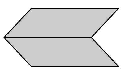
Figure 1: An ambiguous drawing: It can be interpreted as a folded paper with its edge inward or outward of the plane of the drawing.

In Fig.1 we present an ambiguous drawing in order to provide a simple example of the utility of the concept of potential consciousness which will be used in describing perception. Notice that our consciousness offers two potential interpretations of this ambiguous figure: We can perceive it as a folded paper with its edge below or above the plane of the drawing. The reader is encouraged (a) first to try to perceive each of these two interpretations separately, and (b) while watching the drawing to try to stick to one of the two interpretations. Notice that the suggestion (b) is difficult to follow because the two different interpretations alternate in perception every few seconds. Therefore, there are two different potential perceptions of this figure, let us say, symbolically 1 and 2, the one in which the edge is below and the one in which the edge is above the plane respectively. If we ask: “what is the actual figure, is one in which the edge is above or below the plane?” The answer to this question is: “neither” or, equivalently, the answer can be also: “both”. This reminds us of the question: “where is the electron in the atom?”

One of the claims of the present paper is that the best way to describe the state of our consciousness between such perceptual events can be written as:

$$|v\rangle=c_{1}|1\rangle+c_{2}|2\rangle=\left(\begin{array}[]{c}c_{1}\\ c_{2}\end{array}\right),$$ (3)

where $|1\rangle$ and $|2\rangle$ denote two orthogonal unit vectors spanning a vector space and the coefficients $c_{1}$, $c_{2}$, in general, are complex numbers. The reason for using this notation (known in physics as Dirac notation) is for a notational convenience which will become clear in the following few steps. The unit vector $|1\rangle$ corresponds to one of the perceptions and the unit vector $|2\rangle$ to the other perception. The vector $|v\rangle$ given by the linear combination in Eq. 3 describes the state of potential consciousness which corresponds to the stimulus which is neither 1 nor 2; it becomes (or it is realized as) 1 or 2 through the event of a particular perception. In a similar sense the process of measurement in quantum theory (which, in the problem discussed here, corresponds to the conscious realization or conscious event) brings into existence a particular “reality” through the so-called wave-function “collapse”. We will see in the following subsection that the coefficients $c_{1}$, $c_{2}$ are related to the likelihood that the state 1 or 2 will be realized at a given time. Notice that, as special cases the state described by Eq. 3 includes the “pure” states 1 and 2, but the state of potential consciousness is neither; it corresponds to the linear combination given by Eq. 3. This vector $|v\rangle$, which corresponds to the state of potential consciousness, changes in time and we will discuss the equation which gives its time evolution in Sec. II.3. When we perceive the stimulus as either 1 or 2, a perceptual event occurs which brings into perception one or the other experience. We may use the expression that, when state (or interpretation) 1 occurs, the state of potential consciousness $|v\rangle$ “collapses” to $|1\rangle$. In order to describe the dynamics of such perceptual or mental events we will use the notion of potential consciousness and we will show that such a tool is very useful in describing the evolution and distribution of dominance durations in binocular rivalry. In order to achieve that, we need an equation to describe the time-evolution of this state. However, before we discuss this, we should introduce a few other prerequisites.

Given two vectors

$$|v\rangle=\left(\begin{array}[]{c}c_{1}\\ c_{2}\end{array}\right),\hskip 21.68121pt|v^{\prime}\rangle=\left(\begin{array}[]{c}c^{\prime}_{1}\\ c^{\prime}_{2}\end{array}\right),$$ (8)

describing two different states of potential consciousness, we define the inner product in a Hilbert space, in the familiar way, as

$$\langle v|v^{\prime}\rangle=(c^{*}_{1},c^{*}_{2})\left(\begin{array}[]{c}c^{\prime}_{1}\\ c^{\prime}_{2}\end{array}\right)\equiv c^{*}_{1}c^{\prime}_{1}+c^{*}_{2}c^{\prime}_{2}.$$ (11)

Notice that in a Hilbert space, the complex conjugate of the first vector in the inner product is used. This allows us to define a norm, a measure, in this space, namely, the inner product of a vector with itself is a positive real number and can be used as the measure of the “length” of the vector. Also notice in the above notation that we may regard the vector $|v^{\prime}\rangle$ as a $2\times 1$ matrix and we may regard the entity $\langle v|\equiv(c^{*}_{1},c^{*}_{2})$ as a $1\times 2$ matrix obtained as the transpose of $|v\rangle$, i.e., by converting its rows into columns and taking the complex conjugate of its elements. In this way, the inner product of two vectors is the matrix multiplication of a $1\times 2$ with a $2\times 1$ matrix as shown in Eq. 11 above. In addition, this justifies the origin of the notation $\langle v|v^{\prime}\rangle$ used for the inner product.

Now, the absolute magnitude of the inner product between two vectors can also be used to measure how “close” to one another these vectors are. For example, two vectors having zero inner product, implies that these two vectors are orthogonal to each other and this is the largest possible difference between two vectors. Two vectors, each normalized to unity (the norm of each of the vectors is 1), with inner product equal to 1, implies that these two vectors are identical. The inner product will be used in the next subsection where we need to compare two states of potential consciousness.

Therefore, in order to provide a description for the process of perception as a mental (as opposed to a physical) process we introduce a state of potential consciousness which includes the potentialities and the likelihoods for all possible conscious experiences. This state evolves in time and it drastically changes by actual conscious events. To describe this mathematically, for the general case, we write the state of potential consciousness as a vector or a linear superposition of all potential events $|i\rangle$, i.e.,

$$|\psi\rangle=\sum_{i=1}^{N}c_{i}|i\rangle=\left(\begin{array}[]{c}c_{1}\\ .\\ .\\ .\\ c_{N}\end{array}\right),$$ (17)

where $c_{i}$ are, in general, complex numbers and they are related to the probability to actualize the event $i$ whose potentiality is represented by the basis vector $|i\rangle$. The set of all possible potential events $|i\rangle$ forms a complete basis in a Hilbert space describing all potential outcomes.

II.2 Operation of Consciousness and observation

The previous example tells us, that the stimuli have in some sense an “unfathomable” existence, or they exist as potentialities, namely, we can not talk about them directly but only of how they are perceived, i.e., after they have been operated upon by the process of conscious perception. The cake is not sweet before we experience the taste produced through the reaction of our sensory apparatus; before it is tasted, it is potentially sweet. Hence, these potentialities can be actualized directly through the action of the corresponding “organ” of perception in the brain. This operation of consciousness called perception or measurement causes an actual experience and an actual conscious event.

The state of potential consciousness becomes an actuality, i.e., a conscious event occurs, through the operation of conscious attention. For example, imagine that you are having dinner with a number of friends in a round table and several conversations between sub-groups take place simultaneously. When you pay attention or participate in one of the discussions, while the other physical stimuli such as voices come to your instruments of perception, these other stimuli fade and you become aware only of the discussion to which you are paying conscious attention. One can voluntarily switch from one conversation to another by making an effort to enhance the probability of having a “collapse” in a particular desired sector of potential events.

In order to describe this operative process of consciousness we conceptualize consciousness (the thinker) as an actor (or operator) which acts on the state of potential consciousness and makes actual one of the various potentialities. For example, consciousness can only perceive change, i.e., differences, variations, alterations. Imagine an observer who had no prior experiences at all and, suddenly, the observer begins to have a stream of experiences. The observer compares his new observation with a bank of prior experiences and this makes observation a comparative process. The comparative character of the perceptual measurement process is also demonstrated by psychophysical evidence for contextual effects Schwartz et al., (2007). Namely, the perception of a target input depends strongly on both its spatial context (what surrounds a given object) and its temporal context (what has been observed in the recent past). At first, this idea that we only observe change, might be difficult to accept because we know that we are able to observe a static object. In actuality, however, we are able to observe the object because of the constant change caused on our retina by the light coming from the object. This change produces an electric potential difference which will cause a neuron to fire. In order to be able to see the same static object “continuously”, the neuron has to be charged anew and when it “fires”, it causes a perception. Therefore, one of the functions or operations of consciousness is to be able to perceive a change. The operator which measures change in space is the differential operator $\nabla$, while the operator which measures temporal changes is $\partial_{t}$ and both act on the state of potential consciousness $|v\rangle$.

However, we need to answer the following fundamental question: how does consciousness see or measure a change in the absence of an a priori content of memory to be used for comparison? What is the standard, or the measure, which consciousness should use in order to measure the new state? Namely, consciousness operates an inquiry (a question) which is represented by a particular operator $\hat{Q}$ (a matrix) which acts on the state of potential consciousness $|v\rangle$ and during this operation a new, transient, state of potential consciousness results which we represent as $|v^{\prime}\rangle=\hat{Q}|v\rangle$ . Only one state from the set of the various potentialities will be actualized after the measurement; which one?

Let us analyze this question in terms of the example given above regarding the ambiguous figure. In this case, consciousness poses the question: Q = “Is the observed in state $|1\rangle$ ?” ($|1\rangle$ and $|2\rangle$ represent the two alternative states corresponding to the alternative percepts observed when observing the folded paper in Fig.1). The projection operator associated with the above inquiry Q is

$$\hat{Q}=\left(\begin{array}[]{cc}1&0\\ 0&0\end{array}\right),$$ (20)

i.e., depending on the state, it acts as follows:

$$(a) \mathrm{if}\hskip 7.22743pt|v\rangle=|1\rangle=\left(\begin{array}[]{c}1\\ 0\end{array}\right),\hskip 7.22743pt\mathrm{then},\hskip 7.22743pt\hat{Q}|1\rangle=|1\rangle,$$ (23)

$$(b) \mathrm{if}\hskip 7.22743pt|v\rangle=|2\rangle=\left(\begin{array}[]{c}0\\ 1\end{array}\right),\hskip 7.22743pt\mathrm{then},\hskip 7.22743pt\hat{Q}|2\rangle=0.$$ (26)

Now, how does consciousness measures the outcome of this inquiry? It has no measure or standard by which to carry out the measurement, other than the state of potential consciousness just before the inquiry, i.e., $|v\rangle$ given by Eq. 11. Namely, the likelihood that the answer to this question is “yes” should be given by the comparison of the state $|v^{\prime}\rangle=\hat{Q}|v\rangle$ with the state $|v\rangle$ itself. Mathematically, this is evaluated by the inner product between theses two potential states, i.e., $\langle v|v^{\prime}\rangle$ and this notation is defined by Eq. 11. As discussed in the previous subsection the inner product measures how close to each other two states of potential consciousness are. Thus, during the mental event or experience or “collapse” of the state of potential consciousness, the expected value of an observable $\hat{Q}$ is

$$\langle\hat{Q}\rangle=\langle v|\hat{Q}|v\rangle.$$ (27)

Namely, this is the probability for the answer to the above inquiry to be “yes”.

II.3 Evolution of potential consciousness

When we consider the time evolution of any vector $|\psi(t)\rangle$ it is useful to define a different set of vectors forming a complete basis of the same Hilbert space. Such a basis set is formed by all the periodic states $|\nu\rangle_{t}$ characterized by frequency $\omega_{\nu}$ (and period $T_{\nu}=2\pi/\omega_{\nu}$), i.e., $|\nu\rangle_{t+T_{\nu}}=|\nu\rangle_{t}$; the time evolution of these states is given by

$$|\nu\rangle_{t}=e^{\pm i\omega_{\nu}t}|\nu\rangle;\hskip 21.68121pt|\nu\rangle=|\nu\rangle_{0},$$ (28)

and we define an operator $\hat{\omega}$ which is a diagonal matrix in the basis $|\nu\rangle$ with eigenvalues $\omega_{\nu}$, i.e.,

$$\hat{\omega}|\nu\rangle=\omega_{\nu}|\nu\rangle.$$ (29)

The matrix $\hat{\omega}$ is Hermitian, namely, $\langle i|\hat{\omega}|j\rangle=(\langle j|\hat{\omega}|i\rangle)^{*}$ because it has real eigenvalues. The time-dependent state of potential consciousness can be expanded in a Fourier transformation as follows:

$$|\psi(t)\rangle=\sum_{\nu}e^{i\omega_{\nu}t}c_{\nu}|\nu\rangle,$$ (30)

where $c_{\nu}$ are Fourier expansion coefficients and, here, the sum is over both negative and positive $\omega_{\nu}$.

Using the definition of $\hat{\omega}$, Eq. 30 can be written as follows:

$$|\psi(t)\rangle=e^{i\hat{\omega}t}\sum_{\nu}c_{\nu}|\nu\rangle,$$ (31)

which implies that

$$|\psi(t)\rangle=e^{i\hat{\omega}t}|\psi(0)\rangle,$$ (32)

and this is equivalent to the following evolution equation:

$$\hat{\omega}|\psi_{t}\rangle=i\partial_{t}|\psi_{t}\rangle.$$ (33)

We have, therefore, transformed our original problem into one in which we seek an operator $\hat{\omega}$ for the particular perception problem at hand. In the example discussed previously $\hat{\omega}$ is a general $2\times 2$ Hermitian matrix.

This is a Schrödinger-like equation of motion describing the dynamics of cognitive processes. Hence, the state of potential consciousness evolves in a similar way as the state vector evolves in standard quantum mechanics Von-Neumann, (1955), namely, as given by Eq. 32 where the time displacement (or evolution operator) $\hat{U}$ is related to the frequency operator $\hat{\omega}=\hat{H}/\hbar$ (where $\hat{H}$ is the Hamiltonian in quantum mechanics and $\hbar$ is Planck’s constant) as follows

$$\hat{U}=e^{i\int_{0}^{t}\hat{\omega}(t^{\prime})dt^{\prime}},$$ (34)

namely, the frequency operator (which in general can change as a function of time) is the generator of infinitesimal translations in time. In our approach, Planck’s constant does not enter in our equation of motion.

Conscious events that occur are identified with the quantum mechanical “collapses” of the wave function, as specified by the orthodox quantum theory and the meaning of this concept was explained in subsection II.1 above. The wave function, between such perceptual events, describes a state of potential consciousness which evolves via the Schrödinger equation. When a perceptual event is observed, where a wave-function “collapse” occurs through the process of measurement, it actualizes the corresponding neural correlate of consciousness (NCC) brain state.

III Application to Binocular Rivalry

III.1 Time evolution of potential consciousness

In binocular rivalry Blake and Logothetis, (2002); Leopold and Logothetis, (1999); Tong, (2003), which is an example of multi-stable perception Orbach et al., (1966), two different images are presented dichoptically to awareness. These two images are the stimuli for two different potential percepts and form the basis vectors in terms of which to express the general state of potential consciousness. The action of consciousness, i.e., through conscious attention, at a higher level causes the perception of a particular potentiality as a real event in consciousness by activating one particular percept. Through this operation of consciousness, the conscious percept (or symbol) acts and activates the corresponding neural correlates of consciousness (NCC) in the nervous system. Furthermore, a sequence of ordered events arise in consciousness as a time series $t_{1},t_{2},...,t_{n}$ , at each one of which a perceptual change occurs and this defines a flow in consciousness.

State vector formulation: For clarity, we begin with the state vector formulation and below, the problem is also discussed using the density matrix formalism for completeness. We imagine two potential states of consciousness denoted as $|1\rangle$ and $|2\rangle$ which correspond to the two states which can be realized in the case of binocular rivalry, which are associated with two distinct NCC brain states. An arbitrary state of potential consciousness will be written as in Eq. 3 with

$$|c_{1}|^{2}+|c_{2}|^{2}=1,$$ (35)

such that, after the process of projection, the probability for either distinct state to become actual, is unity. Therefore, in binocular rivalry, we have two rival states of consciousness associated with percepts $|1\rangle$ and $|2\rangle$ which, in turn, correspond to two different NCC states.

For binocular rivalry, and more generally for a two-state problem $\hat{\omega}$ is a $2\times 2$ matrix,

$$\hat{\omega}=\left(\begin{array}[]{cc}\langle 1|\hat{\omega}|1\rangle&\langle 1|\hat{\omega}|2\rangle\\ \langle 2|\hat{\omega}|1\rangle&\langle 2|\hat{\omega}|2\rangle\end{array}\right)=\left(\begin{array}[]{cc}\epsilon_{1}&h_{12}\\ h_{21}&\epsilon_{2}\end{array}\right).$$ (40)

As discussed in Sec. II.3, the operator $\hat{\omega}$ must be a Hermitian operator, therefore, $h_{21}=h_{12}^{*}$. To simplify the problem, let us consider, the case where $\epsilon_{1}=\epsilon_{2}=\epsilon$ (namely, the two rival states are “degenerate”, i.e., there is no preference for or bias against one or the other).

In order to solve Eq. 33 in the case where $\hat{\omega}$ is time-independent, we generally proceed Von-Neumann, (1955); Bohm, (1979) by finding the eigenvalues $\omega_{\nu}$ and the eigenstates $|\nu\rangle$ of the operator $\hat{\omega}$ and by expanding the initial state $|\psi(0)\rangle$ in the basis formed by the eigenstates, i.e.,

$$|\psi(0)\rangle=\sum_{\nu}c_{\nu}|\nu\rangle,$$ (41)

and the general time-dependent solution is given by Eq. 30.

Let us suppose that the initial state is just one of the two states, for example state $|1\rangle$. As long as there is no observation (conscious or involuntary attempts to project), the state of potential consciousness as a function of time is in a state given as follows:

$$|\psi_{t}\rangle=\cos(\bar{\omega}t)|1\rangle-ie^{-i\phi}\sin(\bar{\omega}t)|2\rangle.$$ (42)

The frequency $\bar{\omega}=|h_{12}|$ and it is given as $\bar{\omega}=2\pi/T$; $T$ is the characteristic period of the instrument of consciousness. The phase $\phi$ characterizes the off-diagonal matrix elements $h_{12}=\bar{\omega}e^{i\phi}$. The diagonal elements $\epsilon$ of $\hat{\omega}$, in the case where $\epsilon_{1}=\epsilon_{2}=\epsilon$, only contribute to an overall phase which has no observable effects.

Let us consider the inquiry Q: “is the observed in state $|1\rangle$?”, which, for the binocular rivalry case, is represented by the same operator $\hat{Q}$ given by Eq. 20. The expected answer to the inquiry Q is obtained by Eq. 27, and by straightforward substitution of Eq. 42 for the state $|\nu\rangle$ we find that:

$$\langle\hat{Q}\rangle=\cos^{2}(\bar{\omega}t).$$ (43)

Density matrix formulation: Now, let us turn our discussion to the formulation of the problem using the density matrix formalism. The density matrix for a general two state system is given by

$$\hat{\rho}=\left(\begin{array}[]{cc}\langle 1|\hat{\rho}|1\rangle&\langle 1|\hat{\rho}|2\rangle\\ \langle 2|\hat{\rho}|1\rangle&\langle 2|\hat{\rho}|2\rangle\end{array}\right)=\left(\begin{array}[]{cc}\rho_{11}&\rho_{12}\\ \rho_{21}&\rho_{22}\end{array}\right).$$ (48)

The equation of motion satisfied by the density matrix operator is

$$i\partial_{t}\hat{\rho}=[\hat{\omega},\hat{\rho}],$$ (49)

where $\hat{\omega}$ is the frequency operator ($\hat{\omega}=\hat{H}/\hbar$) given by Eq. 40 for the binocular rivalry case. A measurement or observation takes place by means of a conscious inquiry which is represented by a projection operator $\hat{Q}$ (i.e., $\hat{Q}^{2}=\hat{Q}$). For our case of the binocular rivalry the projection operator is given by Eq. 20. The result of a measurement is given as

$$\langle\hat{Q}\rangle=\frac{{Tr(\hat{\rho}\hat{Q})}}{{Tr(\hat{\rho})}}.$$ (50)

If after such a measurement occurs and the answer is “yes” the state of potential consciousness is represented by a density matrix which equals the above projection operator $\hat{Q}$. If after the measurement is “no” the state of potential consciousness is represented by a density matrix given by $\hat{1}-\hat{Q}$.

Let us assume that at time $t=0$ the state of potential consciousness corresponds to the state $|1\rangle$, i.e., to a density matrix $\hat{\rho}=\hat{Q}$. It is straightforward to show that the density matrix $\hat{\rho}(t)$, which satisfies the equation of motion (49) for any time $t$, is given by

$$\hat{\rho}=\left(\begin{array}[]{cc}\cos^{2}(\bar{\omega}t)&-i\sin(\bar{\omega}t)cos(\bar{\omega}t)\\ i\sin(\bar{\omega}t)cos(\bar{\omega}t)&\sin^{2}(\bar{\omega}t)\end{array}\right).$$ (53)

By substituting this expression for the density matrix in Eq. 50 and using the expression given by Eq. 20 for the operator $\hat{Q}$, we obtain the same result for $\langle\hat{Q}\rangle$ as in Eq. 43 above.

III.2 Measurement/projection in Binocular Rivalry

In order for an event to enter the stream of consciousness, a projection/measurement (see Sec. II.2 in the introduction of this paper) must occur. Let us now assume that after time $\delta t$ an observation or measurement is carried out where the state of consciousness is observed by operating (operationally asking) the question Q: “is the observed in state $|1\rangle$?”

This is asked by applying the operator $\hat{Q}=|1\rangle\langle 1|$ (Eq. 20) on the state of potential consciousness $|\psi_{t}\rangle$ and the probability to observe the state $|1\rangle$ is given by $\langle\psi_{t}|\hat{Q}|\psi_{t}\rangle=\cos^{2}(\bar{\omega}\delta t)$ (See Eq. 43). The operation of the inquiry on the state of potential consciousness actualizes the state $|1\rangle$ (or $|2\rangle$) with probability $\cos^{2}(\bar{\omega}\delta t)$ (or $\sin^{2}(\bar{\omega}\delta t/T)$). If $\delta t<<T/4$ there is high probability to observe the state $|1\rangle$. Therefore, if we keep making conscious or involuntary attempts to observe frequently, the same state is projected (the quantum Zeno effect).

We will assume that in an interval $0<t<t_{max}$ a series of observing events occur each one of which causes the neurons to fire in bursts as illustrated in Fig. 2. Let us assume that the observations take place at time instants $t_{1},t_{2},...,t_{n},...,$ and these instances have been picked from a given distribution, an example of which is given in Fig. 2. The probability that the initial state during the first $i-1$ observations at the instances $t_{1},t_{2},...,t_{i-1}$ was repeatedly found to be $|1\rangle$ and found to switch to $|2\rangle$ at time $t_{i}$, is

$$w_{i}=\sin^{2}(\bar{\omega}(t_{i}-t_{i-1}))\prod_{j=1}^{i-1}\cos^{2}(\bar{\omega}(t_{j}-t_{j-1}))).$$ (54)

In this case the dominance duration of the initial state is $t_{i}$. Therefore, the probability density of dominance duration $t$ is given as $P(t)=\sum_{i=1}^{n}w_{i}\delta(t-t_{i})$. This probability density can be calculated using a random walk Monte Carlo process where the time instants of the measurement events $t_{1}$, $t_{2}$,…,$t_{n}$, are chosen from a desired distribution similar to that of Fig. 2. One simple choice of such a sampling technique is to select the first $N_{f}$ events which constitute the first burst as $t_{i}=t_{i-1}+\delta t$ (with $t_{0}=0$) where the variable $\delta t$ is chosen from a Gaussian distribution with variance $T_{f}$ (or as a random variable uniformly distributed in the interval $[0,T_{f}]$). Similarly, the beginning of the next burst is chosen from a Gaussian distribution with variance $T_{b}$ (or as a uniform random variable in the interval $[0,T_{b}]$). A sample train of three such bursts produced using Gaussian distributions with $T_{f}=5msec$, $N_{f}=60$ and $T_{b}=0.9sec$ is shown in Fig. 2.

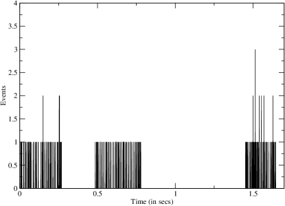
Figure 2: Illustration of the neuronal activity or measurement events needed to understand the distribution of dominance duration in binocular rivalry. Notice that there are the following time scales. (a) A long time scale $T_{b}$, the average time between neuronal firing bursts, (b) the duration of the burst $\delta T$, and (c) the average firing rate $r_{f}=1/T_{f}$ within each burst. Notice that $T_{b}$ is of the order of 1 sec, $\delta T$ is a fraction of a second and $f_{s}$ of the order of $100Hz$. Engel et al., (1992); Gray, (1994); Gray and Singer, (1989); Singer and Gray, (1995)

In Section IX(Appendix) we present a detailed study of this model and how the results differ by changing the neuron firing rates.

IV Results and comparison with experiment

IV.1 Probability distribution of dominance duration

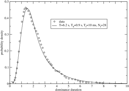
Figure 3: Comparison with the data from Lehky is made using $T=6.2sec$, $T_{b}=0.9sec$ and $T_{f}=10msec$ and $N_{f}=28$ (only the combination $\delta T=T_{f}N_{f}=0.28sec$ is relevant).

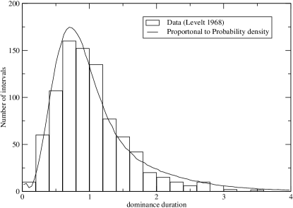
Figure 4: Comparison with the data from Levelt using $T_{b}=0.5$, $\delta T=0.1$, and $T=3$. Time in Ref. Levelt, (1968) is in units of the mean dominance duration. The time scale $T$ is the period characterizing the evolution of the state of potential consciousness (See Section II.3).

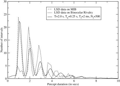
Figure 5: Comparison of the theoretical distribution of dominance duration (solid line) with the data from subjects under the influence of the hallucinogen LSD. The theoretical curve is obtained using $T=2.0sec$, $T_{b}=0.25sec$ and $\delta T=T_{f}N_{f}=1sec$.

In Fig. 3, the distribution of dominance duration obtained using the present model is compared with the data obtained by Lehky Lehky, (1995) and in Fig. 4 it is compared with the data obtained by Levelt Levelt, (1968). The values of the parameters used in the fit, which are given in the figure captions, are reasonable. Neuron firing frequencies of the order of $100Hz$ have been used in these calculations. As discussed in the appendix the probability distribution of dominance duration is not sensitive to the precise value of the spike frequency as long as the burst duration is kept constant. Namely, by varying the spike frequency by even a factor of two or more (within the observed range of neuron firing frequency for the mammalian brain Fries et al., (2002)) and keeping the burst duration constant, we obtain the same probability distribution of dominance duration. The value of the frequency $T$ is determined by setting the scale of time for the graph; the other parameters, which define the neuron firing pattern, are the average time between bursts $T_{b}$ and the burst duration $\delta T$ and their values are consistent with the neuron firing pattern observed for the alert cat Engel et al., (1992); Gray and Singer, (1989); Singer and Gray, (1995). The firing pattern of single cells in the striate cortex of macaque monkeys Martinez-Conde et al., (2000) indicate similar neuron firing patterns. The firing patterns might be somewhat different for neurons of the human cerebral or extra striate cortex, which is the case of our interest; therefore, the values found, in order to achieve good agreement with the observed PDDD, are reasonable.

The value of the oscillation period $T$ is of similar magnitude to a value known as a characteristic time scale for a low-frequency mechanism that binds successive events into perceptual units Pöppel, (1997); Peterson and Peterson, (1959). In a study of the human auditory sensory system by examining the mismatch negativity (MMN) using SQUID magnetometry Sams et al., (1993) it was found that the amplitude of the MMN as a function of the inter-stimulus interval becomes large at a time scale of the order of $3sec$. More recently direct functional MRI measurements Tong et al., (1998); Lumer et al., (1998); Polonsky et al., (2000); Tong and Engel, (2001) demonstrate that the perceived alteration is accompanied by responses in extra-striate cortex areas which are characterized by such time scales. In addition, oscillations at such very low frequencies which correspond to a fraction of a $Hz$ have been observed in EEG patterns during the deep stages of sleep of humans Achermann and Borbely, (1997); Hobson, (2005); Ferri et al., (2005) and of the cat cerebral cortex Destexhe et al., (1999).

In studies Carter and Pettigrew, (2003) with a subject who took the hallucinogenic drug LSD an oscillatory behavior of the distribution of dominance duration was revealed. In Fig. 5, the distribution obtained for the case of binocular rivalry and motion-induced blindness (MIB) from the subject under the influence of LSD is compared with the present model when we use the values of the parameters shown in the inset. Therefore, we conclude that, within the context of our model, the hallucinogenic drug changes the burst frequency and the characteristic period $T$ significantly, which places the observing conscious apparatus into a regime where oscillations are transparent. More recent studies on the influence of hallucinogenic drugs Carter et al., (2005, 2007) indicate that it might be in the “rebound-phase” (a phase reached several hours after the peak of the drug influence) that a state of the type indicated in Fig. 5 and in Ref. Carter and Pettigrew, (2003) may be realized and that this state may not be related at all to the state of consciousness reached at the peak of the LSD influence. More specifically, in Ref. Carter et al., (2005), it was found that the response of subjects at the peak of the drug influence was found to be significantly slower; however, switches for all subjects became increasingly faster, such that six hours later some subjects were switching at intervals that were shorter, more regular and more rhythmic than their pretest levels. Therefore, this is also consistent with the results of Ref. Carter and Pettigrew, (2003) where the subject was tested many hour later than the peak of the drug influence.

We would like to comment about the so-called weak quantum theory (WQT) Atmanspacher et al., (2002) which is an attempt to generalize the formal framework of quantum theory in such a way that complementarity and entanglement might be useful in a broader context. The WQT has been used to describe ambiguous perception Atmanspacher et al., (2004, 2008). There are the following important differences between the present work and WQT and its applications Atmanspacher et al., (2004, 2008): (a) The formalism used in the present paper to describe the dynamics of the mental processes, is identical to that of orthodox quantum theory and we found no need to resort to some other mathematical foundation in the present paper. In addition, there are important differences between the two mathematical models, as applied to the problem of multi-stable perception, namely between the application of WQT and our work. (b) In the present paper the problem of binocular rivalry is studied rather than the problem of ambiguous perception.

IV.2 Periodic removal of stimulus

Next, we discuss the results of Ref. Leopold et al., (2002) where the stimulus was periodically removed as shown in Fig. 6. Namely, the stimulus appears and disappears periodically and both rival images are presented to awareness for a time interval $T_{on}$, and for a time interval $T_{off}$ both images are removed. It was found that the frequency of perceptual alterations can be slowed down, and even brought to almost a standstill. These experimental results are very important because they provide clear support for the present theory.

Here, we are dealing with a frequency operation and a time-evolution operator which changes with time as measured by an external clock. Namely, the frequency operator is given by a constant operator $\hat{\omega}(t)=\hat{\omega}$ (which is a $2\times 2$ matrix), in the on-stimulus time intervals and $\hat{\omega}(t)=0$ in the off-stimulus intervals. When the rival images are presented, the evolution occurs according to the frequency operator $\hat{\omega}$ given by Eq. 40 and when they are totally absent the frequency operator is a constant $C$ (which can be taken to be zero). The general solution of the Schrödinger-like equation, when $\hat{\omega}(t)$ is time dependent, is given by $|\psi_{t}\rangle=e^{i\int_{0}^{t}dt^{\prime}\hat{\omega}(t^{\prime})}|\psi_{0}\rangle$, which implies that $|\psi(t)\rangle$ in the on-stimulus intervals evolves as before and during the off-stimulus interval the state of potential consciousness “freezes”.

In Fig. 7 the probability distribution of the dominance duration is shown. Notice that the probability distribution which corresponds to continuous presentation of the stimulus (solid line), splits into separate parts (gray-shaded) with duration $T_{on}$, when the stimulus is presented intermittently. However, if we eliminate these blank intervals (as if they did not exist) and the separate parts are placed side by side, the result is the same as the distribution obtained with continuous presentation of the stimulus. This result has a number of consequences and we would like to mention the following two: (a) For fixed $T_{on}$, the average dominance duration grows linearly with the blank duration $T_{off}$. (b) For fixed blank duration $T_{off}$, the average dominance duration decreases with increasing $T_{on}$. These conclusions agree well with the available experimental results Orbach et al., (1966); Leopold et al., (2002).

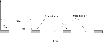
Figure 6: The periodic switching on and off of the rival stimuli. The rival figures are dichoptically presented to awareness for an interval $T_{on}$ and they are removed for a blank interval $T_{off}=T_{ext}-T_{on}$ where $T_{ext}$ is the period of the externally modulated stimulus. Random observations take place during the on-intervals with an average frequency $f_{s}=1/T_{s}$.

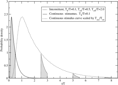
Figure 7: Probability distribution of dominance duration in binocular rivalry with intermittent stimulus. The average time between bursts $T_{b}/T$ is taken to be $0.1$ and the width of the burst is $\delta t/T=0.05$. (a) Solid line: Continuous stimulus. (b) Gray-shaded: Intermittent presentation of stimulus. (c) Doted-line: The distribution of part (a) where the time axis is scaled by a factor $(T_{on}+T_{off})/T_{on}$.

We would like to note that when the stimulus turns on after the blank duration, the change itself is expected to cause a measurement. Our simulation shows that, if at the beginning of the “stimulus on” periods we always start with a burst of $N_{f}$ measurements and the bursts which follow this initial burst are selected according to the same probability distribution, there is additional broadening of the distribution, thus, further increasing the dominance duration. In this case the above mentioned features (a) and (b) are only approximately valid.

V Discussion

The present explanation of the phenomenon observed, when the stimulus was periodically removed, is based on the fact that our theory places the attention of consciousness higher, in the hierarchy of consciousness, than the two stimulated neural correlates in the brain. If we interrupt the external process which presents to awareness the mixture of the two potential states, the state of potential consciousness remains (as memory, with no oscillatory evolution) on the most recently collapsed percept; namely, because of the interruption of the external stimulation of the rival state, there is no reason for alterations of the state of potential consciousness because there is no likelihood associated with the other percept. Therefore, when a new stimulation occurs, where both conscious symbols are presented to awareness, evolution of the state of potential consciousness begins starting from the previously collapsed state. Thus, shortly afterwards, the state of potential consciousness will collapse again in the previously collapsed state with high probability. Hence, when the external presentation to awareness of the stimulus is halted, the time evolution of the state of potential consciousness stops, and the perceived time stands still.

Role of Attention: There are recent studies Ooi and He, (1999); Mitchell et al., (2004); Chong and Blake, (2005) where attention can bias the initial selection of state in binocular rivalry toward the attended state (or stimulus). In our formulation attention is a fundamental aspect of consciousness. Attention is the voluntary or involuntary preparation of the state of potential consciousness with increased likelihood, which causes biased preference, for a certain event or events to occur. If the initial state of potential consciousness is prepared in such a way to be the state $|1\rangle$, this state will be a preferred state when an event occurs soon afterwards.

There are two types of factors which can enhance attention. 1) Bottom-up factors: If we make the diagonal terms of the operator $\hat{\omega}$ different, the probability distribution of dominance durations for state $|1\rangle$ and for $|2\rangle$ would be equal. However, the transition rates would be smaller, a fact that prolongs dominance durations (because there is a potential barrier to be crossed for the oscillations to occur). This is in agreement with the experimental conclusions Chong et al., (2005); Meng and Tong, (2004). 2) Top-down factors: Instructing the observer to pay attention to one particular perceptual state influences and modulates the frequency of measurements. When one eye’s stimulus is strengthened (e.g. by increasing contrast), the mean dominance duration of the other (unaffected) eye decreases Levelt, (1968). In this case the rate of observations $f_{s}$ is different for each of the two eyes. The contrast difference causes the “observer” to increase the rate of observations of one of the states when that state is being experienced.

VI The issue of decoherence

If we consider the formalism of quantum theory as a mathematical foundation that describes the microscopic world, it is very difficult to make a convincing argument that the brain dynamics is governed by quantum theory because of the issue of decoherence Zeh, (1970); Joos and Zeh, (1985); Giulini et al., (1996); Tegmark, (2000). In this work, however, we argued that quantum theory is a broader foundation and it can describe the subjective experience of our thought process and more generally, the perception process. We have reasoned that we can use the formalism of quantum mechanics to describe the testimony of observers where their subjective experience is recorded.

Taking this work seriously, we may postulate that the formalism of quantum theory primarily describes the process of perception and thought. According to such an approach, the reason for the applicability of quantum theory in the microscopic phenomena is because the character of our interaction with the microscopic world can be viewed in the same way as was done here for the case of the perception/thought process. The stimuli from the external world reach our consciousness only through the application of the abstract process of thought and perception Von-Neumann, (1955). Therefore, in order to describe the external world as it is perceived by our conscious apparatus, we need to treat it using the same formulation used to describe the process of perception and thought. Otherwise we would use two different ways of describing our interaction with the external stimuli and this would be inconsistent.

The experimental activity to determine the properties of matter at the atomic or subatomic level can be regarded as an application of the process of perception and thought through the elaborate extension of our sensory apparatus, i.e., using the experimental instruments which are made using the thought process. The questions we ask, when probing the microscopic world, are based on mentally conceived notions while the “object of observation” behaves as “stimulus” to the observing device which is an extension to our sensory apparatus. Furthermore, when we operationally apply our mental constructs through the observing instruments to the microscopic world, they cause significant effects on the nature of the outcome of the perception or measurement process. Namely, the nature of the questions raised in this case have a determining effect on the observed and, this clearly forces us to use more explicitly and more clearly the formalism which describes the process of the operation of thought and perception. Classical mechanics is just a limit of quantum theory when the perturbation caused on the observed as a result of the measurement process is relatively small.

Therefore, in order to describe the operation of consciousness and of thought one does not have to explain how the decoherence is avoided in the brain Tegmark, (2000). This becomes an issue only in the case where one believes that quantum theory is a theory only describing microscopic particles and, thus, when one tries to explain the brain activity starting from such a belief it is difficult to understand how decoherence effects do not become important. Here, however, a very different argument is used, namely, that the mental/abstract process of thought and consciousness is mathematically described by the formalism of quantum theory as described in Sec. II; the fact that the formalism of quantum theory is applicable in the microscopic world follows from this assertion. According to this scenario, in order to describe the process of throught using the formalism of quantum theory, we do not need to identify microscopic processes and to show that they survive the effects of environmental decoherence. It is simply the wrong basis, the wrong level to begin in order to describe the operation of consciousness.

VII Conclusions

In summary, the present theory accurately describes: (a) the distribution of dominance duration in binocular rivalry; (b) the qualitative change in distribution of dominance duration and the appearance of oscillations in subjects which were studied under the influence of hallucinogenic drugs which, as is found, increase the neuron firing rates and decrease the potential frequency; (c) the marked increase in dominance duration by periodic removal of the stimulus.

Furthermore, for binocular rivalry experiments where the stimulus is periodically removed, a distribution of perceptual alterations as a function of time is predicted and this can be tested in future experiments.

VIII Acknowledgements

I wish to thank Henry Stapp for very illuminating discussions. In addition, thanks are due to Sean Barton for proof-reading the manuscript and to Stanley Klein and Olivia Carter for their critical comments.

IX Appendix

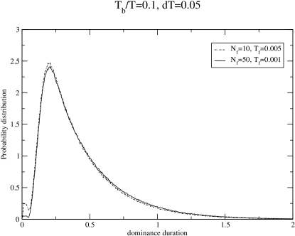
Figure 8: Comparison of $P(t)$ obtained for different firing rates but keeping the duration of firing and everything else constant.

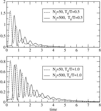
Figure 9: Comparison of $P(t)$ obtained for $T_{f}/T=0.001$ and $N_{f}=50$ and $N_{f}=500$. Top: $T_{b}/T=0.5$. Bottom $T_{b}/T=1.0$.

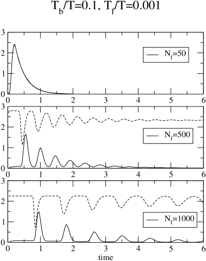
Figure 10: Comparison of $P(t)$ obtained for $T_{b}/T=0.1$ and $T_{f}/T=0.001$. Top: $N_{f}=50$. Middle: $N_{f}=500$. Bottom: $N_{f}=1000$.

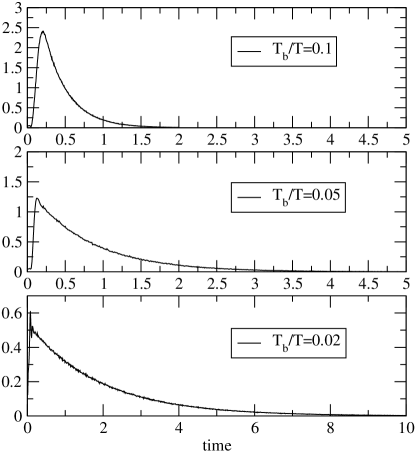
Figure 11: Comparison of $P(t)$ obtained for different small values of $T_{b}/T$ (0.1 (top), 0.05 (center), and 0.02 (bottom)) for $T_{f}/T=0.005$ and $N_{f}=10$. The decay time constant increases by decreasing $T_{b}$. Notice the difference in the scale of time used in the graphs.

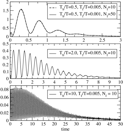
Figure 12: Comparison of $P(t)$ obtained for different values of $T_{b}/T$ (0.5 (top), 2.0 (center), and 10 (bottom)) for $T_{f}/T=0.005$ and $N_{f}=10$. Notice the difference in the scale of time used in the plots.

In this appendix we study the role of the parameters which control the neuron firing rates and the various qualitative different regimes of the present model.

In Fig. 8 we study the effect of changing the firing frequency within any given burst. Therefore we keep the other parameters, namely, the average interval between the end of a burst and the beginning of the next burst $T_{b}/T=0.1$ and the burst duration $\delta T\equiv N_{f}T_{f}=0.1$, fixed. Notice that if we change the number of measurements (which result to neuron firings) within each burst from 10 to 50 the calculated probability distribution of dominance duration $P(t)$ changes significantly only for $0<t\leq\delta T$. This means that when the average interval between measurements is reduced the probability for perceptual change is significantly reduced. The reason for that change is the so-called quantum Zeno effect. This can be easily understood if we consider that the measurements are done at equally spaced intervals $\delta t=\delta T/N_{f}$. The expression given for the transition probability gives

$$P_{N_{f}}(t)=(\cos(\bar{\omega}\delta T/N_{f}))^{2N_{f}}\sin^{2}(\bar{\omega}\delta T/N_{f})$$ (55)

and for large $N_{f}$ the leading term is

$$P_{N_{f}\to\infty}(t)=\Bigl{(}\frac{{\bar{\omega}\delta T}}{{N_{f}}}\Bigr{)}^{2}.$$ (56)

In Fig. 9 and Fig. 10 we demonstrate the effect of increasing the burst duration $\delta T$. We need to distinguish two regimes:

1. When $\delta T\leq T_{b}$. In Fig. 9 it is demonstrated that, by increasing $N_{f}$ from 50 to 500, the initial interval where $P(t)$ is small (of the order of that given by Eq. 56) is extended and it is of the order of $\delta T$. The oscillatory behavior of the function $P(t)$ which is controlled by the period $T$ is unchanged but with the onset delayed by $\delta T$.

2. When $\delta T>T_{b}$, as in the example of Fig. 10. In this case an increase of $\delta T$ leads to an oscillatory behavior with period given approximately by $\delta T$. In Fig. 10 (middle and bottom) the dashed line is the average measurement probability density. Notice the oscillatory behavior of the measurement probability density matches the oscillatory behavior of $P(t)$.

In Fig. 11 the function $P(t)$ calculated for small values of $T_{b}/T$ (and $\delta T/T=0.05$) is plotted. The function $P(t)$ for large $t$ decays exponentially with a decay time constant which increases by decreasing $T_{b}$ as in the quantum Zeno case.

In Fig. 12 the function $P(t)$ calculated for larger values of $T_{b}/T$ (and $\delta T/T=0.05$) is plotted. The function $P(t)$ is oscillating with period $T$ and with envelop of the oscillation decays exponentially with a decay time constant which increases by increasing $T_{b}$.

References

- Achermann and Borbely, (1997) Achermann, P. and Borbely, A. A. (1997). Low frequency ( hz) oscillations in the human sleep electroencephalogram. Neurosci., 81(1):213.
- Atmanspacher et al., (2008) Atmanspacher, H., Bach, M., Filk, T., Kornmeier, J., and Roemer, H. (2008). Cognitive time scales in a necker-zeno model for bistable perception. Open Cybernetics and Systemics Journal, 2:234–251.
- Atmanspacher et al., (2004) Atmanspacher, H., Filk, T., and Roemer, H. (2004). Quantum zeno features of bistable perception. Biol. Cybern., 90:33.
- Atmanspacher et al., (2002) Atmanspacher, H., Roemer, H., and Walach, H. (2002). Weak quantum theory: complementarity and entanglement in physics and beyond. Found. Phys., 32:379.
- Blake and Logothetis, (2002) Blake, R. and Logothetis, N. (2002). Visual competition. Nature Rev. Neurosci., 3:13.
- Bohm, (1979) Bohm, D. (1979). Quantum Mechanics. Dover, New York.
- Carter and Pettigrew, (2003) Carter, O. I. and Pettigrew, J. D. (2003). A common oscillator for perceptual rivalries? Perception, 32:295.
- Carter et al., (2007) Carter, O. L., Hasler, F., Pettigrew, J. D., Wallis, G. M., Liu, G. B., and Vollenweider, F. X. (2007). Psilocybin links binocular rivalry switch rate to attention and subjective arousal levels in humans. Psychopharmacology, 195:415–424.
- Carter et al., (2005) Carter, O. L., Pettigrew, J. D., Hasler, F., Wallis, G. M., Liu, G. B., Hell, D., and Vollenweider, F. X. (2005). Modulating the rate and rhythmicity of perceptual rivalry alternations with the mixed 5-ht2a and 5-ht1a agonist psilocybin. Neuropsychopharmacology, 30:1154.
- Chong and Blake, (2005) Chong, S. C. and Blake, R. (2005). Exogenous and endogenous attention influence initial dominance in binocular rivalry. J. Vision, 5(8):1045a.
- Chong et al., (2005) Chong, S. C., Tadin, D., and Blake, R. (2005). Endogenous attention prolongs dominance durations in binocular rivalry. J. Vision, 5:1004.
- Destexhe et al., (1999) Destexhe, A., Conteras, D., and Steriade, M. (1999). Spatiotemporal analysis of local field potentials and unit discharges in cat cerebral cortex during natural wake and sleep states. J. Neurosci., 19(11):4595.
- Engel et al., (1992) Engel, A. K., Konig, P., Kreiter, A., Schillen, T. B., and Singer, W. (1992). Temporal coding in the visual cortex: new vistas on integration in the nervous system. Trends Neurosci., 15:218.
- Ferri et al., (2005) Ferri, R., Bruni, O., Miano, S., Plazzi, G., and Terzano, M. G. (2005). All-night eeg power spectral analysis of the cyclic alternating pattern components in young adult subjects. Clin. Neurophys., 116:2429.
- Freeman, (2005) Freeman, A. W. (2005). Multistage model for binocular rivalry. J. Neurophysiol., 94:4412.
- Fries et al., (2002) Fries, P., Schröder, J.-H., Roelfsema, P. R., Singer, W., and Engel, A. K. (2002). Oscillatory neuronal synchronization in primary visual cortex as a correlate of stimulus selection. J. Neurosci., 22:3739.
- Giulini et al., (1996) Giulini, D., Joos, E., Kieffer, C., Kupsch, J., Stamatescu, I. O., and Zeh, H. D. (1996). Decoherence and the Appearance of a Classical World in Quantum Theory. Springer New York.
- Gray, (1994) Gray, C. M. (1994). Synchronous oscillations in neuronal systems: Mechanisms and functions. J. Comp. Neurosci., 1:11–38.
- Gray and Singer, (1989) Gray, C. M. and Singer, W. (1989). Stimulus-specific neuronal oscillations in orientation columns of cat visual cortex. Proc. Natl. Acad. Sci. USA, 86:1698.
- Hobson, (2005) Hobson, J. A. (2005). Sleep is of the brain, by the brain and for the brain. Nature, 437:1254.
- Joos and Zeh, (1985) Joos, E. and Zeh, H. D. (1985). The emergence of classical properties through interaction with the environment. Z. Phys., B59:223–243.
- Jung and Pauli, (2001) Jung, C. G. and Pauli, W. (2001). Atom and the Archetype: Pauli/Jung Letters, 1932-1958. ed. C. A. Meier, (Princeton University Press, Princeton).
- Lehky, (1995) Lehky, S. R. (1995). Binocular rivalry is not chaotic. Proc, R, Soc, Lond., B 259:71.
- Leopold and Logothetis, (1999) Leopold, D. A. and Logothetis, N. K. (1999). Multistable phenomena: changing views in perception. Trends of Cogn. Sci., 3:254.
- Leopold et al., (2002) Leopold, D. A., Wilke, M., Mair, A., and Logothetis, N. (2002). Stable perception of visually ambiguous patterns. Nature Neurosci., 5:605.
- Levelt, (1968) Levelt, W. J. M. (1968). Psychological Studies on Binocular Rivalry. Mouton, Hague.
- London and Bauer, (1983) London, F. and Bauer, E. (1983). Quantum Theory and Measurement. J. A. Wheeler and W. H. Zurek eds., pg 217 (Princeton University Press, Princeton).
- Lumer et al., (1998) Lumer, E. D., Friston, K. J., and Rees, G. (1998). Neural correlates of perceptual rivalry in the human brain. Science, 280:1930.
- Manousakis, (2006) Manousakis, E. (2006). Founding quantum theory on the basis of consciousness. Found. Phys., 36(6):795.
- Martinez-Conde et al., (2000) Martinez-Conde, S., Macknik, S. L., and Hubel, D. H. (2000). Microsaccadic eye movements and firing of single cells in the striate cortex of macaque monkeys. Nature Neurosci, 3:251.
- Mavromatos and Nanopoulos, (1998) Mavromatos, N. E. and Nanopoulos, D. V. (1998). On quantum mechanical aspects of microtubules. J. Mod. Phys., B 12:517.
- Meng and Tong, (2004) Meng, M. and Tong, F. (2004). Can attention selectively bias bistable perception? differences between binocular rivalry and ambiguous figures. J. Vision, 4:539–551.
- Mitchell et al., (2004) Mitchell, J. F., Stoner, G. R., and Reynolds, J. H. (2004). Object-based attention determines dominance in binocular rivalry. Nature, 429:410.
- Ooi and He, (1999) Ooi, T. L. and He, Z. J. (1999). Binocular rivalry and visual awareness: The role of attention. Perception, 28:551.
- Orbach et al., (1966) Orbach, J., Zucker, E., and Olson, R. (1966). Reversibility of the necker cube vii. reversal time as a function of figure-on and figure-off durations. Perceptual and Motor Skills, 22:615.
- Penrose, (1989) Penrose, R. (1989). The emperor’s new mind. Oxford University Press, NY.
- Peterson and Peterson, (1959) Peterson, L. R. and Peterson, M. J. (1959). Shortterm retention of individual verbal items. J. Exp. Psychol., 58(3):193.
- Polonsky et al., (2000) Polonsky, A., Blake, R., Braun, J., and Heeger, D. J. (2000). Neuronal activity in human primary visual cortex correlates with perception during binocular rivalry. Nat. Neurosci., 3(11):1153.
- Pöppel, (1997) Pöppel, E. (1997). A hierarchical model of temporal perception. Trends Cognit. Sci., 1:56–61.
- Sams et al., (1993) Sams, M., Hari, R., Rif, J., and Knuutila, J. (1993). The human auditory sensory memory trace persists about 10 sec: neuromagnetic evidence. J. Cogn. Neurosci., 5(3):363.
- Schroedinger, (1967) Schroedinger, E. (1967). What is life? and Mind and Matter. Cambridge University Press, Cambridge.
- Schwartz et al., (2005) Schwartz, J. M., Stapp, H. P., and Beauregard, M. (2005). Quantum physics in neuroscience and psychology: a neurophysical model of mind-brain interaction. Phil. Tran. Royal Soc., B 360(1458):1306.
- Schwartz et al., (2007) Schwartz, O., Hsu, A., and Dayan, P. (2007). Space and time in visual context. Nature Rev. Neurosci., 8:522.
- Singer and Gray, (1995) Singer, W. and Gray, C. M. (1995). Visual feature integration and the temporal correlation hypothesis. Annu. Rev. Neurosci., 18:555.
- Stapp, (1980) Stapp, H. P. (1980). Locality and reality. Found. Phys., 10:767.
- Stapp, (2003) Stapp, H. P. (2003). Mind, Matter and Quantum Mechanics. Springer-Verlag, Berlin.
- Stapp, (2007) Stapp, H. P. (2007). Mindful Universe: Quantum Mechanics and the Participaring Observer. Springer-Verlag, Berlin.
- Tegmark, (2000) Tegmark (2000). The importance of quantum decoherence in brain processes. Phys. Rev. E., 61:4194–4206.
- Tong, (2003) Tong, F. (2003). Primary visual cortex and visual awareness. Nature Rev. Neurosci., 4:219.
- Tong and Engel, (2001) Tong, F. and Engel, S. A. (2001). Interocular rivalry revealed in the human cortical blind-spot representation. Nature, 411:195.
- Tong et al., (2006) Tong, F., Meng, M., and Blake, R. (2006). Neural bases of binocular rivalry. Trends Cogn Sci, 10:512.
- Tong et al., (1998) Tong, F., Nakayama, K., Vaughan, J. T., and Kanwisher, N. (1998). Binocular rivalry and visual awareness in human extrastriate cortex. Neuron, 21:753.
- Von-Neumann, (1955) Von-Neumann, J. (1955). Mathematical Foundations of Quantum Mechanics, Chap. VI, pg. 417. Princeton University Press, Princeton.
- Wigner, (1983) Wigner, E. P. (1983). Quantum Theory and Measurement. J. A. Wheeler and W. H. Zurek eds., pg 260 and 325 (Princeton University Press, Princeton).
- Zeh, (1970) Zeh, H. D. (1970). Toward a quantum theory of observation. Found. Phys., 1:69–76.