Faddeev calculation of pentaquark $\Theta^{+}$
in the Nambu-Jona-Lasinio model-based
diquark picture

Abstract

A Bethe-Salpeter-Faddeev (BSF) calculation is performed for the pentaquark $\Theta^{+}$ in the diquark picture of Jaffe and Wilczek in which $\Theta^{+}$ is a diquark-diquark-${\bar{s}}$ three-body system. Nambu-Jona-Lasinio (NJL) model is used to calculate the lowest order diagrams in the two-body scatterings of ${\bar{s}}D$ and $DD$. With the use of coupling constants determined from the meson sector, we find that ${\bar{s}}D$ interaction is attractive in $s$-wave while $DD$ interaction is repulsive in $p$-wave. With only the lowest three-body channel considered, we do not find a bound $\frac{1}{2}^{+}$ pentaquark state. Instead, a bound pentaquark $\Theta^{+}$ with $\frac{1}{2}^{-}$ is obtained with a unphysically strong vector mesonic coupling constants.

1 Introduction

The report of the observation of a very narrow peak in the $K^{+}n$ invariant mass distribution [1, 2] around 1540 MeV in 2003, a pentaquark predicted in a chiral soliton model [3], triggered considerable excitement in the hadronic physics community. It has been labeled as $\Theta^{+}$ and included by the PDG in 2004 [4] under exotic baryons and rated with three stars. Very intensive research efforts, both theoretically and experimentally, ensued.

On the experimental side, practically all studies conducted after the first sightings were confirmed by several other groups produced null results, casting doubt on the existence of the five-quark state [5, 6]. Subsequently, PDG in 2006 reduced the rating from three to one stars [4]. More recently, the ZEUS experiment at HERA [7] observed a signal for $\Theta^{+}$ in a high energy reaction, while H1 [7], SPHINX [8] and CLAS [9] did not see it. This disagreement between the LEPS [1] and other experiments could possibly originate from their differences of experimental setups and kinematical conditions. So the experimental situation is presently not completely settled [10, 11, 12].

Many theoretical approaches have been employed, in addition to the chiral soliton model [3], including quark models [13], QCD sum rules [15], and lattice QCD [16] to understand the properties and structure of $\Theta^{+}$. Several interesting ideas were also proposed on the pentaquark production mechanism. Review of the theoretical activities in the last couple of years can be found in Refs. [17, 18].

One of the most intriguing theoretical ideas suggested for $\Theta^{+}$ is the diquark picture of Jaffe and Wilczek (JW) [19] in which $\Theta^{+}$ is considered as a three-body system consisted of two scalar, isoscalar, color $\bf{\bar{3}}$ diquarks ($D$’s) and a strange antiquark $(\bar{s})$. It is based, in part, on group theoretical consideration. It would hence be desirable to examine such a scheme from a more dynamical perspective.

The idea of diquark is not new. It is a strongly correlated quark pair and has been advocated by a number of QCD theory groups since 60’s [20, 21, 22]. It is known that diquark arises naturally from an effective quark theory in the low energy region, the Nambu-Jona-Lasinio (NJL) model [23, 24]. NJL model conveniently incorporates one of the most important features of QCD, namely, chiral symmetry and its spontaneously breaking which dictates the hadronic physics at low energy. Models based on NJL type of Lagrangians have been very successful in describing the low energy meson physics [25, 26]. Based on relativistic Faddeev equation the NJL model has also been applied to the baryon systems [27, 28]. It has been shown that, using the quark-diquark approximation, one can explain the nucleon static properties reasonably well [29, 30]. If one further take the static quark exchange kernel approximation, the Faddeev equation can be solved analytically. The resulting forward parton distribution functions [31] successfully reproduce the qualitative features of the empirical valence quark distribution. The model has also been used to study the generalized parton distributions of the nucleon [32]. Consequently, we will employ NJL model to describe the dynamics of a diquark-diquark-antiquark system. To describe such a three-particle system, it is necessary to resort to Faddeev formalism.

Since the NJL model is a covariant-field theoretical model, it is important to use relativistic equations to describe both the three-particle and its two-particle subsystems. To this end, we will adopt Bethe-Salpeter-Faddeev (BSF) equation [33] in our study. For practical purposes, Blankenbecler-Sugar (BbS) [34] reduction scheme will be followed to reduce the four-dimensional integral equation into three-dimensional ones.

In Sec II, NJL model in flavor $SU(3)$ will be introduced with focus on the diquark. The NJL model is then used to investigate the antiquark-diquark and diquark-diquark interaction with Bethe-Salpeter equation in Sec. III. In Sec. IV, we introduce the Bethe-Salpeter-Faddeev equation and solve it for the system of strange antiquark-diquark-diquark with the interaction obtained in Sec. III. Results and discussions are presented in Sec. V, and we summarize in Sec. VI.

2 $\bf SU(3)_{f}$ NJL model and the diquark

The flavor $SU(3)_{f}$ NJL Lagrangian takes the form

$${\cal L}={\bar{\psi}}(i\mbox{$\!\not\!\partial$}-m)\psi+{\cal L}_{I},$$ (1)

where $\psi^{T}=(u,d,s)$ is the SU(3) quark field, and $m=diag(m_{u},m_{d},m_{s})$ is the current quark mass matrix. ${\cal L}_{I}$ is a chirally symmetric four-fermi contact interaction. By a Fierz transformation, we can rewrite ${\cal L}_{I}$ into a Fierz symmetric form ${\cal L}_{I,q{\bar{q}}}=\frac{1}{2}({\cal L}_{I}+{\cal F}({\cal L}_{I}))$, where ${\cal F}$ stands for the Fierz rearrangement. It has the advantage that the direct and exchange terms give identical contribution.

In the $q{\bar{q}}$ channel, the chiral invariant ${\cal L}_{I,q{\bar{q}}}$, is given by [35]

$${\cal L}_{I,q{\bar{q}}} = G_{1}\left[({\bar{\psi}}\lambda^{a}_{f}\psi)^{2}-({\bar{\psi}}\gamma^{5}\lambda^{a}_{f}\psi)^{2}\right]-G_{2}\left[({\bar{\psi}}\gamma^{\mu}\lambda^{a}_{f}\psi)^{2}+({\bar{\psi}}\gamma^{\mu}\gamma^{5}\lambda^{a}_{f}\psi)^{2}\right]$$ (2)

$$- G_{3}\left[({\bar{\psi}}\gamma^{\mu}\lambda^{0}_{f}\psi)^{2}+({\bar{\psi}}\gamma^{\mu}\gamma^{5}\lambda^{0}_{f}\psi)^{2}\right]-G_{4}\left[({\bar{\psi}}\gamma^{\mu}\lambda^{0}_{f}\psi)^{2}-({\bar{\psi}}\gamma^{\mu}\gamma^{5}\lambda^{0}_{f}\psi)^{2}\right]$$

$$+ \cdots,$$

where $a=0\sim 8$, and $\lambda_{f}^{0}=\sqrt{\frac{2}{3}}I$. If we define $G_{5}$ by $-G_{5}({\bar{\psi}}_{i}\gamma^{\mu}\psi_{j})^{2}=-(G_{2}+G_{3}+G_{4})({\bar{\psi}}_{i}\gamma^{\mu}\lambda^{0}_{f}\psi_{j})^{2}-G_{2}({\bar{\psi}}_{i}\gamma^{\mu}\lambda^{8}_{f}\psi_{j})^{2}$ where $i,j=u,d$, then $G_{3},G_{4},G_{5}$ are related by $G_{5}=G_{2}+\frac{2}{3}G_{v},$ with $G_{v}\equiv G_{3}+G_{4}.$ In passing, we mention that the conventionally used $G_{\omega}$ and $G_{\rho}$ are related to $G_{5},G_{v}$ by $G_{\omega}=2G_{5}$ and $G_{\rho}=2G_{5}-\frac{4}{3}G_{v}$.

For the diquark channel we rewrite ${\cal L}_{I}$ into an form $({\bar{\psi}}A{\bar{\psi}}^{T})(\psi^{T}B\psi)$, where $A$ and $B$ are totally antisymmetric matrices in Dirac, isospin and color indices. We will restrict ourselves to scalar, isoscalar diquark with color and flavor in $\bf\bar{3}$ as considered in the JW model. The interaction Lagrangian for the scalar-isoscalar diquark channel [36, 37] is given by

$${\cal L}_{I,s}=G_{s}\left[{\bar{\psi}}(\gamma^{5}C)\lambda_{f}^{2}\beta^{A}_{c}{\bar{\psi}}^{T}\right]\left[\psi^{T}(C^{-1}\gamma^{5})\lambda_{f}^{2}\beta^{A}_{c}\psi\right],$$ (3)

where $\beta^{A}_{c}=\sqrt{\frac{3}{2}}\lambda^{A}(A=2,5,7)$ corresponds to one of the color ${\bar{3}}_{c}$ states. $C=i\gamma^{0}\gamma^{2}$ is the charge conjugation operator, and $\lambda^{\prime}s$ are the Gell-Mann matrices.

The Bethe-Salpeter (BS) equation for the scalar diquark channel [36, 37] is given by

$$\tau_{s}(q)=4iG_{s}-2iG_{s}\int\frac{d^{4}k}{(2\pi)^{4}}tr[(C^{-1}\gamma^{5}\tau_{f}^{2}\beta^{A}))S(k+q)(\gamma^{5}C\tau_{f}^{2}\beta^{A})S^{T}(-q)]\tau_{s}(q),$$ (4)

where the factors $4$ and $2$ arise from Wick contractions. $S(k)=(\mbox{$\!\not\!k$}-M+i\epsilon)^{-1}$ with $M\equiv M_{u}=M_{d}$, the constituent quark mass of u and d quarks, generated by solving the gap equation. $\tau_{s}(q)$ is the reduced t-matrix which is related to the t-matrix by $t_{s}(q)=(\gamma^{5}C\tau_{f}^{2}\beta^{A}_{c})\tau_{s}(q)(C^{-1}\gamma^{5}\tau_{f}^{2}\beta^{A}_{c})$. The solution to Eq. (4) is

$$\tau_{s}(q)=\frac{4iG_{s}}{1+2G_{s}\Pi_{s}(q^{2})},$$ (5)

with

$$\Pi_{s}(q^{2})=6i\int\frac{d^{4}k}{(2\pi)^{4}}tr_{D}[\gamma^{5}S(q)\gamma^{5}S(k+q)].$$ (6)

The gap equation for u, d and s quarks are given by

$$M_{i}=m_{i}-8G_{1}<{\bar{q}}_{i}q_{i}>,$$ (7)

with

$$<{\bar{q}}_{i}q_{i}>\equiv-iN_{c}\int\frac{d^{4}k}{(2\pi)^{4}}tr_{D}(S(k)),$$ (8)

where $i=u,d,s$.

The loop integrals in Eqs. (6) and (8) diverge and we need to regularize the four-momentum integral by adopting some cutoff scheme. With regularization, we can solve the gap equation and t-matrix of the diquark in Eqs. (5) and (8) to determine the constituent quark and diquark masses. However, since our purpose in this work is not an exact quantitative analysis but rather a qualitatively study of the interactions inside $\Theta^{+}$, we will not adopt any regularization scheme and simply use the empirical values of the constituent quark masses $M=M_{u,d}=400$ MeV, $M_{s}=600$ MeV, and the diquark mass $M_{D}=600$ MeV as obtained in the study of the nucleon properties [27, 28, 29, 31, 32].

3 Two-body interactions for strange antiquark-diquark $(\bf\bar{s}D)$ and diquark-diquark ($DD$) channels

In the JW model for $\Theta^{+}$, the two scalar-isoscalar, color $\bf\bar{3}$ diquarks must be in a color $\bf 3$ in order to combine with $\bar{s}$ into a color singlet. Since $\bf 3$ is the antisymmetric part of $\bf\bar{3}\times\bar{3}=3\oplus\bar{6}$, the diquark-diquark wave function must be antisymmetric with respect to the rest of its labels. For two identical scalar-isoscalar diquarks $[ud]_{0}$, only spatial labels remain so that the spatial wave function must be antisymmetric under space exchange and the lowest possible state is $p$-state. Since in JW’s scheme, $\Theta^{+}$ has the quantum number of $J^{P}={\frac{1}{2}}^{+}$, $\bar{s}$ would be in relative $s$-wave to the $DD$ pair. Accordingly, we will consider only the configurations where $\bar{s}D$ and $DD$ are in relative $s$- and $p$-waves, respectively.

We will employ Bethe-Salpeter-Faddeev equation [33] to describe such a three-particle system of $\bar{s}DD$. For consistency, we will use Bethe-Salpeter equation to describe two-particles subsystems like $\bar{s}D$ and $DD$, which reads as,

$$T=B+BG_{0}T,$$ (9)

where B is the sum of all two-body irreducible diagrams and $G_{0}$ is the free two-body propagator. In momentum space, the resulting Bethe-Salpeter equation can be written as

$$T(k^{\prime},k;P)=B(k^{\prime},k;P)+\int d^{4}k^{{}^{\prime\prime}}B(k^{\prime},k^{{}^{\prime\prime}};P)G_{0}(k^{{}^{\prime\prime}};P)T(k^{{}^{\prime\prime}},k;P),$$ (10)

where $G_{0}$ is the free two-particle propagator in the intermediate states. $k$ and $P$ are, respectively, the relative and total momentum of the system.

In practical applications, B is commonly approximated by the lowest order diagrams prescribed by the model Lagrangian and will be denoted by V hereafter. In addition, it is often to further reduce the dimensionality of the integral equation (10) from four to three, while preserving the relativistic two-particle unitarity cut in the physical region. It is well known (for example, Ref. [38]) that such a procedure is rather arbitrary and we will adopt, in this work, the widely employed Blankenbecler-Sugar (BbS) reduction scheme [34] which, for the case of two spinless particles, amounts to replacing $G_{0}$ in Eq. (10) by

$$G_{0}(k,P) = \frac{1}{(P/2+k)^{2}-m_{1}^{2}}\frac{1}{(P/2-k)^{2}-m_{2}^{2}}$$ (11)

$$\rightarrow -i(2\pi)^{4}\frac{1}{(2\pi)^{3}}\int\frac{ds^{\prime}}{s-s^{\prime}+i\epsilon}$$

$$\times \delta^{(+)}\left((P^{\prime}/2+k)^{2}-m_{1}^{2}\right)\delta^{(+)}\left((P^{\prime}/2-k)^{2}-m_{2}^{2}\right)$$

$$= -2\pi i\delta\left(k_{0}-\frac{E_{1}(|\vec{k}|)-E_{2}(|\vec{k}|)}{2}\right)G^{BbS}(|\vec{k}|,s),$$

with

$$G^{BbS}(|\vec{k}|,s)=\frac{E_{1}(|\vec{k}|)+E_{2}(|\vec{k}|)}{2E_{1}(|\vec{k}|)E_{2}(|\vec{k}|)}\frac{1}{s-(E_{1}(|\vec{k}|)+E_{2}(|\vec{k}|))^{2}+i\epsilon},$$ (12)

where $s=P^{2}$ and $P^{\prime}=\sqrt{s^{\prime}/s}P$. The superscript (+) associated with the delta functions mean that only the positive energy part is kept in the propagator, and $E_{1,2}(|\vec{k}|)\equiv\sqrt{\vec{k}^{2}+m_{1,2}^{2}}$.

3.1 $\bf{\bar{s}}$D potential and the t-matrix

In Fig. 1 we show the lowest order diagram, i.e., first order in ${\cal L}_{I,q{\bar{q}}}$ in ${\bar{s}}D$ scattering. Due to the trace properties for Dirac matrices, only the scalar-isovector $({\bar{\psi}}\lambda^{a}_{f}\psi)^{2}$, the vector-isoscalar $({\bar{\psi}}\gamma^{\mu}\lambda^{0}_{f}\psi)^{2}$, and the vector-isovector $({\bar{\psi}}\gamma^{\mu}\lambda^{a}_{f}\psi)^{2}$ will contribute to the vertex $\Gamma$.

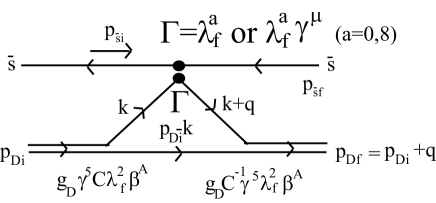
Figure 1: ${\bar{s}}$D potential of the lowest order in ${\cal L}_{I,q{\bar{q}}}$.

Furthermore, the isovector vertex $(\bar{\psi}\Gamma\lambda_{f}^{a}\psi)^{2}$ will not contribute since the trace in flavor space vanishes, $\sum_{a=0}^{8}(\lambda_{f}^{a})_{33}tr_{f}(\lambda_{f}^{2}\lambda_{f}^{a}\lambda_{f}^{2})=0$. Thus only the vector-isoscalar term, $({\bar{\psi}}\gamma^{\mu}\lambda^{0}_{f}\psi)^{2}$, remains.

For the on-shell diquarks, the lower part of Fig. 1 which corresponds to the scalar diquark form factor, can be calculated as

$$(p_{Di}+p_{Df})^{\mu}F_{v}(q^{2}) = i\int\frac{d^{4}k}{(2\pi)^{4}}tr[(g_{D}C^{-1}\gamma^{5}\lambda_{f}^{2}\beta^{A}_{c})S(k+q)\gamma^{\mu}S(k)(g_{D}\gamma^{5}C\lambda_{f}^{2}\beta^{A}_{c})S^{T}(k-p_{Di})]$$ (13)

$$= 6ig_{D}^{2}\int\frac{d^{4}k}{(2\pi)^{4}}tr[S(k+q)\gamma^{\mu}S(k)S(p_{Di}-k)],$$

where we have made use of the relations $C^{-1}(\gamma^{\mu})^{T}C=-\gamma^{\mu}$, $tr_{c}[\beta^{A}_{c}\beta^{A}_{c}]=3$. $g_{D}$ is defined by

$$g_{D}^{-2}=-\left.\frac{\partial\Pi_{D}(p^{2})}{\partial p^{2}}\right|_{p^{2}=M_{D}^{2}},$$ (14)

with

$$\Pi_{D}(p^{2})\equiv 6i\int\frac{d^{4}k}{(2\pi)^{4}}tr[S(k)S(p-k)],$$ (15)

and $M_{D}$ is the diquark mass. $F_{v}(0)$ is normalized as $2p^{\mu}F_{v}(0)=-g_{D}^{2}\frac{\partial\Pi_{D}(p^{2})}{\partial p_{\mu}}$, such that $F_{v}(0)=1$.

Then the matrix element of the potential $V_{\bar{s}D}$ can be expressed as

$$<{\bar{s}}_{f}D_{f}|V|{\bar{s}}_{i}D_{i}> = (-{\bar{v}}(p_{{\bar{s}}i}))(-iV_{{\bar{s}}D})(p_{Di},p_{Df})v(p_{{\bar{s}}f})$$ (16)

$$= (+16i)(-G_{v})(-{\bar{v}}(p_{{\bar{s}}i}))\gamma_{\mu}v(p_{{\bar{s}}f})\left[(\lambda^{0}_{f})_{33}\cdot tr_{f}\left(\lambda^{0}_{f}(\lambda_{f}^{2})^{2}\right)\right]$$

$$\times (p_{Di}+p_{Df})^{\mu}\frac{F_{v}(q^{2})}{tr_{f}((\lambda_{f}^{2})^{2})},$$

i.e.,

$${V}_{{\bar{s}}D}=\frac{64}{3}G_{v}F_{v}(q^{2})\tilde{V}_{{\bar{s}}D}(p_{Di},p_{Df}),$$ (17)

with

$$\tilde{V}_{{\bar{s}}D}({p}_{Di},{p}_{Df})=(\mbox{$\!\not\!p$}_{Di}+\mbox{$\!\not\!p$}_{Df})/2.$$ (18)

Here the factor $+16i$ in Eq. (16) arises from the Wick contractions, and the factor $tr_{f}((\lambda_{f}^{2})^{2})$ in Eq. (16) is introduced to divide $F_{v}(q^{2})$, since the factor $tr_{f}((\lambda_{f}^{2})^{2})$ is already included in the expression of $F_{v}(q^{2})$ by a trace in flavor $SU(3)_{f}$ space.

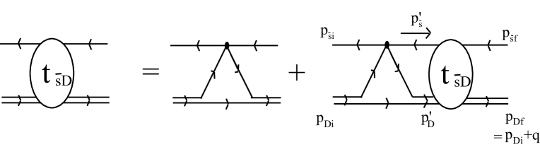
Figure 2: The BS equation for ${\bar{s}}$D.

The three-dimensional scattering equation for the ${\bar{s}}D$ system is now given by

$$t_{{\bar{s}}D}(p_{Di},p_{Df}) = V_{{\bar{s}}D}(p_{Di},p_{Df})$$

$$+ 4\pi\int\frac{d|\vec{p}^{\,\,{}^{\prime}}_{D}||\vec{p}^{\,\,{}^{\prime}}_{D}|^{2}}{(2\pi)^{3}}\frac{1}{2}\int_{-1}^{1}dx_{i}G_{{\bar{s}}D}^{BbS}(|\vec{p}^{\,\,{}^{\prime}}_{D}|,s_{2})K_{{\bar{s}}D}(|\vec{p}_{Di}|,|\vec{p}^{\,\,{}^{\prime}}_{D}|,x_{i})t_{{\bar{s}}D}(\vec{p}^{\,\,{}^{\prime}}_{D},p_{Df}),$$

where $x_{i}\equiv\hat{p}_{Di}\cdot\hat{p}_{D}^{\,\,{}^{\prime}}$, $\hat{p}\equiv\vec{p}/|p|$, $s_{2}=(p_{Di}+p_{{\bar{s}}i})^{2}=(p_{Df}+p_{{\bar{s}}f})^{2}$, $p_{Di}^{0}=\sqrt{\vec{p}_{Di}^{\,\,2}+M_{D}^{2}}$, $p_{Df}^{0}=\sqrt{\vec{p}_{Df}^{\,\,2}+M_{D}^{2}}$ and

$$K_{{\bar{s}}D}(|\vec{p}_{Di}|,|\vec{p}^{\,\,{}^{\prime}}_{D}|,x_{i}) \equiv \frac{64}{3}G_{v}F_{v}((p^{\prime}_{D}-p_{Di})^{2})\tilde{K}_{{\bar{s}}D}(p_{Di},p^{\prime}_{D})|_{{p^{\prime}_{D}}^{0}=\sqrt{{\vec{p}}^{\,\,{}^{\prime}2}_{D}+M_{D}^{2}}},$$

$$\tilde{K}_{{\bar{s}}D}(p_{Di},p^{\prime}_{D}) = (\mbox{$\!\not\!p$}_{Di}+\mbox{$\!\not\!p$}_{D}^{\,\,{}^{\prime}})(-\mbox{$\!\not\!p$}_{\bar{s}}^{\,\,{}^{\prime}}+M_{s})/2,$$

with $M_{s}$ being the constituent quark mass of ${\bar{s}}$ and $s$.

We also present the results for the interactions between diquark and $\bar{u}$ or $\bar{d}$, which would be of interest when we study non-strange pentaquarks. One can just repeat the derivations we describe in the above and easily obtain

$${V}_{{\bar{u}}D}={V}_{{\bar{d}}D}=\\ -16G_{1}F_{s}(q^{2})+32G_{5}F_{v}(q^{2})\tilde{V}_{{\bar{s}}D}(p_{Di},p_{Df}),$$ (20)

in analogous to Eqs. (17) and (18).

We add in passing that, within tree approximation, the sign of the potential for $sD$ is opposite to that of $V_{{\bar{s}}D}$ due to charge conjugation, i.e.,

$$V_{sD}(p_{Df},p_{Di})=-V_{{\bar{s}}D}(p_{Di},p_{Df}).$$ (21)

We can immediately write down the scattering equation for the $sD$ as,

$$t_{sD}(p_{Df},p_{Di}) = V_{sD}(p_{Df},p_{Di})$$

$$+ 4\pi\int\frac{d|\vec{p}^{\,\,{}^{\prime}}_{D}||\vec{p}^{\,\,{}^{\prime}}_{D}|^{2}}{(2\pi)^{3}}\frac{1}{2}\int_{-1}^{1}dx_{f}G_{sD}^{BbS}(|\vec{p}^{\,\,{}^{\prime}}_{D}|,s_{2})K_{sD}(|\vec{p}_{Df}|,|\vec{p}^{\,\,{}^{\prime}}_{D}|,x_{f})t_{sD}(\vec{p}^{\,\,{}^{\prime}}_{D},p_{Di}),$$

where $x_{f}\equiv\hat{p}_{Df}\cdot\hat{p}_{D}^{\,\,{}^{\prime}}$, $G_{sD}^{BbS}(|\vec{p}^{\,\,{}^{\prime}}_{D}|,s_{2})=G_{{\bar{s}}D}^{BbS}(|\vec{p}^{\,\,{}^{\prime}}_{D}|,s_{2})$, and

$$K_{sD}(|\vec{p}_{Df}|,|\vec{p}^{\,\,{}^{\prime}}_{D}|,x_{f}) \equiv \frac{64}{3}G_{v}F_{v}((p^{\prime}_{D}-p_{Df})^{2})\tilde{K}_{sD}(p_{Df},p^{\prime}_{D})|_{{p^{\prime}_{D}}^{0}=\sqrt{{\vec{p}}^{\,\,{}^{\prime}2}_{D}+M_{D}^{2}}},$$

$$\tilde{K}_{sD}(p_{Df},p^{\prime}_{D}) = -(\mbox{$\!\not\!p$}_{Df}+\mbox{$\!\not\!p$}_{D}^{\,\,{}^{\prime}})(\mbox{$\!\not\!p$}_{s}^{\,\,{}^{\prime}}+M_{s})/2,$$ (23)

with $p^{\prime}_{s}=p^{\prime}_{\bar{s}}$.

3.2 Representation in $\rho$-spin notation

In the ${\bar{s}}D$ (or $sD$) center of mass system the wave function which describes the relative motion in $J=\frac{1}{2}$, is given by the Dirac spinor of the following form (see [39, 40]),

$$\Psi_{sD,m_{s}}(p_{s}^{0},\vec{p}_{s}) = \left(\begin{array}[]{c}\phi_{s1}(p_{s}^{0},|\vec{p}_{s}|)\\ \vec{\sigma}\cdot\hat{p}_{s}\,\phi_{s2}(p_{s}^{0},|\vec{p}_{s}|)\\ \end{array}\right)\chi_{m_{s}},$$ (26)

$$\Psi_{{\bar{s}}D,m_{s}}(p_{\bar{s}}^{0},\vec{p}_{\bar{s}}) = \left(\begin{array}[]{c}\vec{\sigma}\cdot\hat{p}_{\bar{s}}\,\phi_{{\bar{s}}2}(p_{\bar{s}}^{0},|\vec{p}_{\bar{s}}|)\\ \phi_{{\bar{s}}1}(p_{\bar{s}}^{0},|\vec{p}_{\bar{s}}|)\\ \end{array}\right)\chi_{m_{s}},$$ (29)

$$= \gamma^{5}\left(\begin{array}[]{c}\phi_{{\bar{s}}1}(p_{\bar{s}}^{0},|\vec{p}_{\bar{s}}|)\\ \vec{\sigma}\cdot\hat{p}_{\bar{s}}\,\phi_{{\bar{s}}2}(p_{\bar{s}}^{0},|\vec{p}_{\bar{s}}|)\\ \end{array}\right)\chi_{m_{s}},$$ (32)

$${\bar{\Psi}}_{sD}(p_{s}^{0},\vec{p}_{s}) \equiv \Psi_{sD}^{\dagger}(p_{s}^{0},\vec{p}_{s})\gamma^{0},$$ (33)

$${\bar{\Psi}}_{{\bar{s}}D}(p_{\bar{s}}^{0},\vec{p}_{\bar{s}}) \equiv \Psi_{{\bar{s}}D}^{\dagger}(p_{\bar{s}}^{0},\vec{p}_{\bar{s}})\gamma^{0},$$ (34)

where $\vec{p}_{D}=-\vec{p}_{s}=-\vec{p}_{\bar{s}}$, i.e., $\Psi_{sD}(p_{s}^{0},\vec{p}_{s})=\Psi_{sD}(p_{s}^{0},-\vec{p}_{D})$ and $\Psi_{{\bar{s}}D}(p_{\bar{s}}^{0},\vec{p}_{\bar{s}})=\Psi_{{\bar{s}}D}(p_{\bar{s}}^{0},-\vec{p}_{D})$. In the following we simply write $p^{\prime}_{Q}=|\vec{p}^{\,\,{}^{\prime}}_{Q}|,p^{\prime}_{Qi(f)}=|\vec{p}^{\,\,{}^{\prime}}_{Qi(f)}|$ , $Q=s,{\bar{s}}$ or $D$. Note that the index 1 (2) corresponds to large (small) components for both ${\bar{s}}$ and $s$ quark spinors.

For a discretization in spinor space, we define the complete set of $\rho$-spin notation ([39, 41]) for the operators ${\cal O}_{sD}=V_{sD},t_{sD},\tilde{V}_{sD}$ and ${\cal K}_{sD}=K_{sD},\tilde{K}_{sD}$ of $sD$:

$${\cal O}_{sD,nm}(p_{Df},p_{Di}) \equiv tr[\Omega^{\dagger}_{n}(p_{sf}){\cal O}_{sD}(p_{Df},p_{Di})\Omega_{m}(p_{si})],$$ (35)

$${\cal K}_{sD,nm}(p_{Df},p_{D}^{\prime},x_{f}) \equiv tr[\Omega^{\dagger}_{n}(p_{sf}){\cal K}_{sD}(p_{Df},p_{D}^{\prime},x_{f})\Omega_{m}(p^{\prime}_{s})],$$ (36)

where $n,m=1,2$, $\Omega_{1}(p)=\frac{\Omega}{\sqrt{2}}$ and $\Omega_{2}(p)=\vec{\gamma}\cdot\hat{p}\frac{\Omega}{\sqrt{2}}$, $\Omega=\frac{1+\gamma_{0}}{2}$. $\Omega_{1}(p)$ and $\Omega_{2}(p)$ satisfy $tr[\Omega^{\dagger}_{n}(p)\Omega_{m}(p^{\prime})]=\delta_{n1}\delta_{m1}+\hat{p}\cdot\hat{p}^{\,\,{}^{\prime}}\delta_{n2}\delta_{m2}$.

Concerning the ${\bar{s}}D$ spinor, the large and small components can be reversed by $\gamma^{5}$, with the minus sign which comes from the definitions Eqs. (32) and (34): ${\bar{\Psi}}_{{\bar{s}}D}{\cal O}\Psi_{{\bar{s}}D}=-{\bar{\Psi}}_{sD}\gamma^{5}{\cal O}\gamma^{5}\Psi_{sD}$. Then we can define $\rho$-spin notation for ${\bar{s}}D$ i.e., ${\cal O}_{{\bar{s}}D}=V_{{\bar{s}}D},t_{{\bar{s}}D},\tilde{V}_{{\bar{s}}D}$ and ${\cal K}_{{\bar{s}}D}=K_{{\bar{s}}D},\tilde{K}_{{\bar{s}}D}$,

$${\cal O}_{{\bar{s}}D,nm}(p_{Di},p_{Df}) \equiv -tr[\Omega^{\dagger}_{n}(p_{{\bar{s}}i})\gamma^{5}{\cal O}_{{\bar{s}}D}(p_{Di},p_{Df})\gamma^{5}\Omega_{m}(p_{{\bar{s}}f})],$$ (37)

$${\cal K}_{{\bar{s}}D,nm}(p_{Di},p_{D}^{\prime},x_{i}) \equiv -tr[\Omega^{\dagger}_{n}(p_{{\bar{s}}i})\gamma^{5}{\cal K}_{{\bar{s}}D}(p_{Di},p_{D}^{\prime},x_{i})\gamma^{5}\Omega_{m}(p_{\bar{s}}^{\prime})].$$ (38)

From Eqs. (LABEL:tsbD,LABEL:tsD,35-38), each component $n$ $(n=1,2)$ of spinors for the ${\bar{s}}$D satisfy the following quadratic equation:

$$\phi^{\dagger}_{{\bar{s}}n}(p_{{\bar{s}}i})t_{{\bar{s}}D,nm}(p_{Di},p_{Df})\phi_{{\bar{s}}m}(p_{{\bar{s}}f})=\phi^{\dagger}_{{\bar{s}}n}(p_{{\bar{s}}i})\Bigl{[}V_{{\bar{s}}D,nm}(p_{Di},p_{Df})$$

$$+4\pi\sum_{l=1}^{2}\int\frac{dp_{D}^{\prime}}{(2\pi)^{3}}p_{D}^{{}^{\prime}2}\frac{1}{2}\int_{-1}^{1}dx_{i}G_{{\bar{s}}D}^{BbS}(p_{D}^{\prime},s_{2})K_{{\bar{s}}D,nl}(p_{Di},p_{D}^{\prime},x_{i})t_{{\bar{s}}D,lm}(p_{D}^{\prime},p_{Df})\Bigr{]}\phi_{{\bar{s}}m}(p_{{\bar{s}}f}).$$

(39)

A similar equation can be obtained for the $sD$ by exchanging $i\leftrightarrow f$ and $s\leftrightarrow{\bar{s}}$ in Eq. (39).

The explicit expressions of the $\rho$-spin notation for $\tilde{V}_{{\bar{s}}(s)D}$ and $\tilde{K}_{{\bar{s}}(s)D}$ are given in appendix B. We note that there are important relations:

$$V_{{\bar{s}}D,nm}(p,q) = -V_{sD,nm}(p,q),$$

$$V_{{\bar{s}}D}(p,q) = -V_{sD}(p,q),$$

$$K_{{\bar{s}}D,nm}(|\vec{p}^{\,}|,|\vec{q\,}|,x_{pq}) = -K_{sD,nm}(|\vec{p}^{\,}|,|\vec{q}^{\,}|,x_{pq}),$$

$$K_{{\bar{s}}D}(|\vec{p}^{\,}|,|\vec{q}^{\,}|,x_{pq}) = -K_{sD}(|\vec{p}^{\,}|,|\vec{q}^{\,}|,x_{pq}).$$

By the partial wave expansion in Eq. (75) in appendix A, the BS equation for $t_{{\bar{s}}D,nm}$ in Eq. (39) for $s$-wave can be written as

$$t_{{\bar{s}}D,nm}^{l_{{\bar{s}}D}=0}(p_{Di},p_{Df})=V_{{\bar{s}}D,nm}^{l_{{\bar{s}}D}=0}(p_{Di},p_{Df})+4\pi\int\frac{dp_{D}^{\,{}^{\prime}}}{(2\pi)^{3}}p_{D}^{\,{}^{\prime}2}\sum_{l=1}^{2}G_{{\bar{s}}D}^{BbS}(p_{D}^{\,{}^{\prime}},s_{2})K^{l_{{\bar{s}}D}=0}_{{\bar{s}}D,nl}(p_{Di},p_{D}^{\,{}^{\prime}})t_{{\bar{s}}D,lm}^{l_{{\bar{s}}D}=0}(p_{D}^{\,{}^{\prime}},p_{Df}).$$ (40)

3.3 $DD$ potential and t-matrix

In the case of $DD$ interaction, the lowest order diagrams are depicted in Figs. 3(a) and (b), with (a) the quark rearrangement diagram and (b) of the first order in ${\cal L}_{I,q\bar{q}}$, respectively.

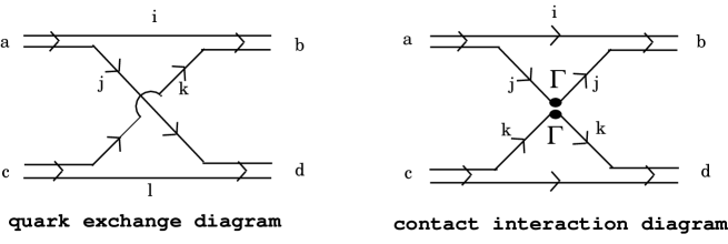
Figure 3: Lowest order diagrams in $DD$ scattering.

We first show that the quark exchange diagram in Fig. 3(a) does not contribute due to its color structure, where $a\sim d$ and $i\sim l$ denote the color indices of the diaquarks and quarks, respectively. Since each diquark is in the color ${\bf\bar{3}}$ [19, 36], the color factor for the $qqD$ vertex is proportional to $\epsilon_{aij}$. Hence the color factor of the quark exchange diagram is given by

$$\epsilon_{aij}\epsilon_{bik}\epsilon_{clk}\epsilon_{dlj}=\delta_{ab}\delta_{cd}+\delta_{ad}\delta_{bc}.$$ (41)

As we discussed earlier, the color of the $DD$ pair inside $\Theta^{+}$ is of ${\bf 3}$ in order to combine with ${\bar{s}}$ to form a color singlet pentaquark. As color ${\bf 3}$ state is antisymmetric under the exchange between diquarks in the initial and final states, the matrix element of Eq. (41) vanishes.

For the contact interaction diagram Fig. 3(b), only the direct term is shown since the exchange term does not contribute as it has the same color structure as the quark rearrangement diagram of Fig 3(a). It is easy to see that the color structure of Fig. 3(b) is proportional to $\delta_{ab}\delta_{cd}$. Then the terms in the interaction Lagrangian in Eq. (2) that can give rise to non-vanishing contributions are:

$$G_{1}({\bar{\psi}}\lambda^{a}_{f}\psi)^{2},\,\,-G_{2}({\bar{\psi}}\gamma^{\mu}\lambda^{a}_{f}\psi)^{2},\,\,-G_{v}({\bar{\psi}}\gamma^{\mu}\lambda^{0}_{f}\psi)^{2},$$ (42)

with $a=0\sim 8$.

We next calculate the form factors, which diagrammatically correspond to the lower part of diagram in Fig. 1. For $\Gamma=\gamma^{\mu}\lambda_{f}^{a}$, we obtain

$${tr_{f}\left(\lambda_{f}^{a}(\lambda_{f}^{2})^{2}\right)}(p_{Di}+p_{Df})^{\mu}\frac{F_{v}(q^{2})}{tr_{f}((\lambda_{f}^{2})^{2})}$$ (43)

$$= \left(\sqrt{\frac{2}{3}}\delta_{a0}+\sqrt{\frac{1}{3}}\delta_{a8}\right)(p_{Di}+p_{Df})^{\mu}F_{v}(q^{2}),$$

and for $\Gamma=\lambda_{f}^{a}$, we get

$${tr_{f}\left(\lambda_{f}^{a}(\lambda_{f}^{2})^{2}\right)}\frac{F_{s}(q^{2})}{tr_{f}((\lambda_{f}^{2})^{2})}\\ =\left(\sqrt{\frac{2}{3}}\delta_{a0}+\sqrt{\frac{1}{3}}\delta_{a8}\right)F_{s}(q^{2}),$$

where the factor ${tr_{f}((\lambda_{f}^{2})^{2})}$ in Eqs. (43) and (3.3) is introduced by the same reason for Eq. (16), and we have used $tr(\lambda_{f}^{2}\lambda_{f}^{a}\lambda_{f}^{2})=2(\sqrt{\frac{2}{3}}\delta_{a0}+\sqrt{\frac{1}{3}}\delta_{a8})$.

For the on-shell diquarks, $F_{s}(q^{2})$ is calculated as

$$F_{s}(q^{2}) = i\int\frac{d^{4}k}{(2\pi)^{4}}tr[(g_{D}C^{-1}\gamma^{5}\lambda_{f}^{2}\beta^{A})S(k+q)S(k)(g_{D}\gamma^{5}C\lambda_{f}^{2}\beta^{A})S^{T}(k-p_{Di})]$$ (44)

$$= 6ig_{D}^{2}\int\frac{d^{4}k}{(2\pi)^{4}}tr[S(k+q)S(k)S(k-p_{Di})].$$

With the form factors $F_{v}(q^{2})$ and $F_{s}(q^{2})$ obtained in the above, $V_{DD}$ is given by

$$-iV_{DD}(\vec{p}_{Di},\vec{p}_{Df}) = +128i\left[G_{1}F_{s}^{2}(q^{2})-\left(G_{2}+\frac{2}{3}G_{v}\right)(p_{D1i}+p_{D1f})\cdot(p_{D2i}+p_{D2f})F_{v}^{2}(q^{2})\right]$$ (45)

$$= 128i\left[G_{1}F_{s}^{2}(q^{2})-G_{5}(p_{D1i}+p_{D1f})\cdot(p_{D2i}+p_{D2f})F_{v}^{2}(q^{2})\right],$$

where the factor $+128i$ in a first line of Eq. (45) comes from the Wick contractions, and in a second line we have used the relation between couplling constants in meson sectors; $G_{5}=G_{2}+\frac{2}{3}G_{v}$ which is explained in section 2. The momenta of the diquarks in the initial and final states in Fig. 4 are given by

$$p_{D1i(f)} = (\sqrt{s_{2}}/2,\vec{p}_{Di(f)}),$$

$$p_{D2i(f)} = (\sqrt{s_{2}}/2,-\vec{p}_{Di(f)}),$$ (46)

with $q=p_{D1f}-p_{D1i}=p_{D2i}-p_{D2f}$. $s_{2}=4(\vec{p}_{Di}^{\,2}+M_{D}^{2})=4(\vec{p}_{Df}^{\,2}+M_{D}^{2})$ is the $DD$ center of mass energy squared.

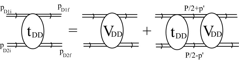
Figure 4: BS equation for $DD$.

As in the case of $\bar{s}D$ scattering, we use the BbS three-dimensional reduction scheme and the resulting equation for $DD$ scattering reads as

$$t_{DD}(\vec{p}_{Df},\vec{p}_{Di})=V_{DD}(\vec{p}_{Df},\vec{p}_{Di})+\int\frac{d^{3}p^{\prime}}{(2\pi)^{3}}V_{DD}(\vec{p}_{Df},\vec{p}^{\,\,{}^{\prime}})G_{DD}^{BbS}(|\vec{p}^{\,\,{}^{\prime}}|,s_{2})t_{DD}(\vec{p}^{\,\,{}^{\prime}},\vec{p}_{Di}),$$ (47)

with

$$G_{DD}^{BbS}(|\vec{p}^{\,\,{}^{\prime}}|,s_{2}) = \frac{1}{4E_{D}(|\vec{p}^{\,\,{}^{\prime}}|)(s_{2}/4-E_{D}(|\vec{p}^{\,\,{}^{\prime}}|)^{2}+i\epsilon)}$$ (48)

$$= \frac{1}{4E_{D}(|\vec{p}^{\,\,{}^{\prime}}|)(\vec{p}_{Df}^{\,\,2}-\vec{p}^{\,\,{}^{\prime}2}+i\epsilon)},$$

with $E_{D}(|\vec{p}^{\,\,{}^{\prime}}|)=\sqrt{\vec{p}^{\,\,{}^{\prime}2}+M_{D}^{2}}$.

In the JW model for $\Theta^{+}$, the diquark-diaquark spatial wave function must be antisymmetric and we will consider here only the lowest configuration, namely, $DD$ are in relative $p$-wave. Partial wave expansion of Eq. (75) then gives

$$t_{DD}^{l=1}(p_{f},p_{i})=V_{DD}^{l=1}(p_{f},p_{i})+4\pi\int\frac{dp^{\prime}}{(2\pi)^{3}}p^{\prime 2}G_{DD}^{BbS}(p^{\prime},s_{2})V_{DD}^{l=1}(p_{f},p^{\prime})t_{DD}^{l=1}(p^{\prime},p_{i}),$$ (49)

with $p_{i(f)}\equiv|\vec{p}_{Di(f)}|,p^{\prime}\equiv|\vec{p}^{\,\,{}^{\prime}}|$.

4 Relativistic Faddeev equation

4.1 3-body Lippmann-Schwinger equation

For a system of three particles with momenta $\vec{k}_{i}^{\prime}s\,(i=1,2,3)$, we introduce the Jacobi momenta with particle 3 as a special choice:

$$\vec{k}_{1} = \mu_{1}\vec{P}+\vec{\tilde{p}}+\alpha_{1}\,\,\vec{\tilde{q}}_{3}$$

$$\vec{k}_{2} = \mu_{2}\vec{P}-\vec{\tilde{p}}+\alpha_{2}\,\,\vec{\tilde{q}}_{3}$$

$$\vec{k}_{3} = \mu_{3}\vec{P}+\alpha_{3}\,\,\vec{\tilde{q}}_{3},$$ (50)

with $\sum\mu_{n}=1$ and $\alpha_{3}=-\alpha_{1}-\alpha_{2}$. For the coefficients we find $\mu_{n}=m_{n}/M$,   $M=m_{1}+m_{2}+m_{3}$,   and $\alpha_{1}=m_{1}/m_{12},\,\,\alpha_{2}=m_{2}/m_{12},\,\,\alpha_{3}=-1$, where $m_{ij}=m_{i}+m_{j}\,\,(i\neq j).$ In terms of the Jacobi momenta the total kinetic energy is given by:

$$K_{tot}=\frac{P^{2}}{2M}+\frac{\tilde{p}\,^{2}}{2m_{12}}+\frac{{\tilde{q}_{3}}^{2}}{2m_{(12)3}},$$ (51)

where $m_{(ij)k}={m_{k}m_{ij}}/{M}$.

New integration variables are chosen to be: $\tilde{p}=f_{p3}\,\,p$ with $f_{p3}=\sqrt{2m_{12}}$ and $\tilde{q_{3}}=f_{q3}\,\,q$ with $f_{q3}=\sqrt{2m_{(12)3}}$, and in general for cyclic $(ijk)$, $f_{pi}=\sqrt{2m_{jk}}$ and $f_{qi}=\sqrt{2m_{(jk)i}}$. In terms of the new integration variables we have

$$K_{tot}=\frac{P^{2}}{2M}+p^{2}+q^{2},$$ (52)

and the 3-body Lippmann-Schwinger equation for the T-matrix becomes:

$$T(\vec{p},\vec{q})=V+{f_{p3}}^{3}{f_{q3}}^{3}\int\,\,\frac{d^{3}p^{\prime}}{(2\pi)^{3}}\int\,\,\frac{d^{3}q^{\prime}}{(2\pi)^{3}}\,\,V\,\,G_{3}(p^{\prime},q^{\prime})\,\,T(\vec{p}\,^{\prime},\vec{q}\,^{\prime}),$$ (53)

with $G_{3}(p,q)=1/(z-K_{tot})$. The parameter $z$ is implicit in the arguments of $T$ and $G_{3}$ in Eq. (53), a convention to be followed hereafter.

Similarly we define the Jacobi momenta $\vec{p}_{i},\vec{q}_{i}$ with particle $i$ as the special choice. The momenta are related to each other as

$$\vec{p}_{i}=a_{ij}\vec{p}_{j}+b_{ij}\vec{q}_{j},\hskip 56.9055pt\vec{q}_{i}=c_{ij}\vec{p}_{j}+d_{ij}\vec{q}_{j},$$ (54)

where $(ijk)$ are cyclic, and $a_{ij}=-[m_{i}m_{j}/(m_{i}+m_{k})(m_{j}+m_{k})]^{1/2}$, $b_{ij}=\sqrt{1-a_{ij}^{2}}=-b_{ji}$, $c_{ij}=-b_{ij}$ and $d_{ij}=a_{ij}$.

It can be shown that the total angular momentum is related to the angular momentum $\vec{l}_{pi}$ and $\vec{l}_{qi}$ by

$$\vec{L}=\sum\limits_{i=1}^{3}{\left({\vec{r}_{i}\times\vec{k}_{i}}\right)}=\sum\limits_{i=1}^{3}{\left({\vec{l}_{pi}+\vec{l}_{qi}}\right)}+\vec{l}_{c}.$$ (55)

With these three choices of Jacobi momenta we may introduce corresponding 3-particle states $|>_{n}$ where particle $n$ plays a special role. For the 3-particle T-matrix we have

$$<\vec{k}_{1},\vec{k}_{2},\vec{k}_{3}|T|\alpha>=_{n}<\vec{p}_{n},\vec{q}_{n}|T|\alpha>,$$ (56)

or in terms of the Faddeev amplitudes $T_{n}$,

$$<\vec{k}_{1},\vec{k}_{2},\vec{k}_{3}|T|\alpha>=T_{1}(\vec{p}_{1},\vec{q}_{1})+T_{2}(\vec{p}_{2},\vec{q}_{2})+T_{3}(\vec{p}_{3},\vec{q}_{3}),$$ (57)

with $T_{n}(\vec{p}_{n},\vec{q}_{n})=_{n}<\vec{p}_{n},\vec{q}_{n}|T_{n}|\alpha>$.

For the pentaquark system we now chose particles 1 and 3 as the diquark and particle 2 to be the ${\bar{s}}$. The Faddeev equations for $T=T_{1}+T_{2}+T_{3}$ with $T_{i}=t_{i}+\sum\limits_{j\neq i}{t_{i}}G_{2}(s)T_{j}\,\,\,(i=1,2,3)$, with $t_{i}$ denoting the two-body t-matrix between particle pair $(jk)$, become

$$T_{1}(\vec{p}_{1},\vec{q}_{1}) = {f_{p3}}^{3}{f_{q3}}^{3}\int\frac{d^{3}p^{\prime}_{3}}{(2\pi)^{3}}\int\frac{d^{3}q^{\prime}_{3}}{(2\pi)^{3}}\,\,K_{13}\,\,G_{3}(p^{\prime}_{3},q^{\prime}_{3})\,\,T_{3}(\vec{p}_{3}\,^{\prime},\vec{q}_{3}\,^{\prime})$$ (58)

$$+ {f_{p2}}^{3}{f_{q2}}^{3}\int\frac{d^{3}p^{\prime}_{2}}{(2\pi)^{3}}\int\frac{d^{3}q^{\prime}_{2}}{(2\pi)^{3}}\,\,K_{12}\,\,G_{3}(p^{\prime}_{2},q^{\prime}_{2})\,\,T_{2}(\vec{p}_{2}\,^{\prime},\vec{q}_{2}\,^{\prime}),$$

where the channels 1 and 3 correspond to $D({\bar{s}}D)$ states and channel 2 to the ${\bar{s}}(DD)$ states. Since diquarks obey Bose-Einstein statistics, we have $T_{3}(\vec{p}_{3},\vec{q}_{3})=T_{1}(-\vec{p}_{3},\vec{q}_{3})$ and $T_{3}(\vec{p}_{3},\vec{q}_{3})=T_{1}(-\vec{p}_{1},\vec{q}_{1})$. We note that the symmetry property which requires the amplitude $T$ be anti-symmetric with respect to interchange of the 2 diquarks is automatically satisfied by the angular momentum content $L=l_{q1}=l_{p2}=1,l_{p1}=l_{q2}=0$.

The ${\bar{s}}(DD)$ T-matrix $T_{2}$ satisfies

$$T_{2}(\vec{p}_{2},\vec{q}_{2})=2fp^{3}_{1}fq^{3}_{1}\int\frac{d^{3}p^{\prime}_{1}}{(2\pi)^{3}}\int\frac{d^{3}q^{\prime}_{1}}{(2\pi)^{3}}\,\,K_{21}\,\,G_{3}({p}_{1}^{\prime},{q}_{1}^{\prime})\,\,T_{1}(\vec{p}_{1}\,^{\prime},\vec{q}_{1}\,^{\prime}).$$ (59)

The kernels $K_{13}$ and $K_{12}$ are expressed in terms of the ${\bar{s}}D$ t-matrix

$$K_{13}=K_{12}=t_{{\bar{s}}D}(\vec{p}_{1},{\vec{p}_{1}}\,^{\prime};z-q_{1}^{2})\,\,\frac{{(2\pi)^{3}}}{f_{q_{1}}\,^{3}}\delta^{(3)}[\vec{q}_{1}-\vec{q}_{1}\,^{\prime}].$$ (60)

Similarly the kernel $K_{21}$ is given by

$$K_{21}=t_{DD}(\vec{p}_{2},\vec{p}_{2}\,^{\prime};z-q_{2}^{2})\,\,\frac{{(2\pi)^{3}}}{f_{q_{2}}\,^{3}}\delta^{(3)}[\vec{q}_{2}-\vec{q}_{2}\,^{\prime}].$$ (61)

The term with $K_{13}$ can be worked out by making use of the $\delta$-function relation

$$\delta^{(3)}\left[{\vec{q}_{1}-{\vec{q}}_{1}\,^{\prime}}\right]=\frac{2}{q_{1}}\delta\left({q_{1}^{2}-{{q}_{1}^{\prime}}^{2}}\right)\delta\left({\cos\theta_{q_{3}}-\cos\theta_{{q}_{3}^{\prime}}}\right)\delta\left({\phi_{{q}_{3}^{\prime}}-\phi_{q_{3}}}\right),$$ (62)

and the linear relation $\vec{q}_{1}\,^{\prime}=c_{13}\vec{p}_{3}\,^{\prime}+d_{13}\vec{q}_{3}\,^{\prime}$, which lead to

$$\delta^{(3)}\left[{\vec{q}_{1}-\vec{q}_{1}\,^{\prime}}\right] = \frac{1}{q_{1}c_{13}d_{13}{p}_{3}^{\prime}{q}_{3}^{\prime}}\delta\left({\cos\theta_{p_{3}^{\prime}q_{3}^{\prime}}-\frac{q_{1}^{\prime 2}-c_{13}^{\prime 2}p_{3}^{\prime 2}-d_{13}^{2}q_{3}^{\prime 2}}{2c_{13}d_{13}p_{3}^{\prime}q_{3}^{\prime}}}\right)$$ (63)

$$\times \delta\left({\cos\theta_{q_{3}}-\cos\theta_{q_{3}^{\prime}}}\right)\delta\left({\phi_{q_{3}^{\prime}}-\phi_{q_{3}}}\right).$$

We mention that similar expression for a delta function in the term $K_{12}$ can also be obtained by replacing $3\rightarrow 2$.

Performing a partial wave expansion for the $D({\bar{s}}D)$ amplitude

$$T_{1}(\vec{p}_{1},\vec{q}_{1})=4\pi Y_{lp_{1}0}^{*}(\Omega_{p_{1}})Y_{lq_{1}0}(\Omega_{q_{1}})T_{1}^{L}(p_{1},q_{1}),$$ (64)

and for the $\bar{s}D$ t-matrix $t_{\bar{s}D}(\vec{p}_{1},\vec{p}_{1}\,^{\prime};z-q_{1}^{2})$,

$$t_{\bar{s}D}(\vec{p}_{1},\vec{p}_{1}\,^{\prime};z-q_{1}^{2})=4\pi{Y_{l{p_{1}}0}^{*}(\Omega_{p_{1}})Y_{lp_{1}0}(\Omega_{p^{\prime}_{1}})}t_{\bar{s}D}^{(l_{p1})}({p}_{1},{p}_{1}^{\prime};z-q_{1}^{2}),$$ (65)

yield

$$T_{1}^{L}(p_{1},q_{1})$$

$$=c_{3}\int_{0}^{\infty}{q^{\prime}_{3}}^{2}dq^{\prime}_{3}\int_{A_{13}}^{B_{13}}{p^{\prime}_{3}}^{2}dp^{\prime}_{3}\,\,t^{(lp_{1})}_{{\bar{s}}D}(p_{1},p^{\prime}_{1};z-q_{1}^{2})\,\,X_{13}\,\frac{1}{c_{13}\,d_{13}\,q_{1}\,p^{\prime}_{3}\,q^{\prime}_{3}}\,\,G_{3}(p^{\prime}_{3},q^{\prime}_{3})\,\,T_{3}^{L}(p^{\prime}_{3},q^{\prime}_{3})$$

$$+c_{2}\int_{0}^{\infty}{q^{\prime}_{2}}^{2}dq^{\prime}_{2}\int_{A_{12}}^{B_{12}}{p^{\prime}_{2}}^{2}dp^{\prime}_{2}\,\,t_{{\bar{s}}D}^{(lp_{1})}(p_{1},p^{\prime}_{1};z-q_{1}^{2})\,\,X_{12}\,\frac{1}{c_{12}\,d_{12}\,q_{1}\,p^{\prime}_{2}\,q^{\prime}_{2}}\,\,G_{3}(p^{\prime}_{2},q^{\prime}_{2})\,\,T_{2}^{L}(p^{\prime}_{2},q^{\prime}_{2}),$$

with

$$c_{3}=\frac{2}{\sqrt{\pi}}({f_{p3}f_{q3}}/{f_{q1}})^{3},\,\,c_{2}=\frac{2}{\sqrt{\pi}}({f_{p2}f_{q2}}/{f_{q1}})^{3},$$ (67)

and where the boundaries $A,B$ for the $p^{\prime}$ integration can easily be found from the condition $q^{2}_{1}={q^{\prime}_{1}}^{2}$ in Eq. (63), given by

$$A_{ij} = \left|\frac{c_{ij}{q}^{\prime}_{j}+q_{i}}{d_{ij}}\right|$$ (68)

$$B_{ij} = \left|\frac{c_{ij}{q}^{\prime}_{j}-q_{i}}{d_{ij}}\right|,$$ (69)

For the ${\bar{s}}(DD)$ amplitude $T_{2}$, partical wave expansion gives,

$$T_{2}^{L}(p_{2},q_{2}) = 2c_{1}\int_{0}^{\infty}{q^{\prime}_{1}}^{2}dq^{\prime}_{1}\int_{A_{21}}^{B_{21}}{p^{\prime}_{1}}^{2}dp^{\prime}_{1}\,\,$$ (70)

$$\times t_{DD}^{(lp_{2})}(p_{2},p^{\prime}_{2};z-q^{2}_{2})\,\,X_{21}\,\,\frac{1}{c_{21}\,d_{21}\,q_{2}\,p^{\prime}_{1}\,q^{\prime}_{1}}\,\,G_{3}(p^{\prime}_{1},q^{\prime}_{1})\,\,T_{1}^{L}(p_{1}^{\prime},q_{1}^{\prime}),$$

where $A_{21}$ and $B_{21}$ are given by Eq. (69), and

$$c_{1}=\frac{2}{\sqrt{\pi}}({f_{p1}f_{q1}}/{f_{q2}})^{3}.$$ (71)

In the above equations $X_{ij}$ are angular momentum functions depending on the states we consider. In our case, the ${\bar{s}}D$ 2-body channel is a s-wave, $lp=0$, and the $DD$ channel a p-wave, $lp=1$. Hence, for the 3-body channel with total angular momentum $L=1$ we have for the $D({\bar{s}}D)$ 3-body channnel $lp_{1}=0,lq_{1}=L$ and $lp_{3}=0,lq_{3}=L$, while for ${\bar{s}}(DD)$ $lp_{2}=1,lq_{2}=0$. The obtained $X_{ij}$ have the form

$$X_{13}=\frac{1}{4\pi\sqrt{3}}Y_{lq_{3}0}(\theta_{q_{3}\,q_{1}}),\,\,X_{12}=\frac{1}{4\pi\sqrt{3}}Y_{lq_{2}0}(\theta_{q_{2}\,q_{1}}),\,\,X_{21}=\frac{1}{4\pi\sqrt{3}}Y_{lp_{2}0}(\theta_{p_{2}\,p_{1}}).$$ (72)

4.2 Relativistic Faddeev equations

Following Amazadeh and Tjon [42] (see also [33]) we adopt the relativistic quasi-potential prescription based on a dispersion relation in the 2-particle subsystem. Then the 3-body Bethe-Salpeter-Faddeev equations have essentially the same form as the non relativistic version.Taking the representation with particle 3 as special choice we may write down for the 3-particle Green function a dispersion relation of the (1,2)-system, i.e.,

$$G_{3}(p_{3},q_{3};s_{3})=\frac{E_{1}(k_{1})+E_{2}(k_{2})}{E_{1}(k_{1})\,E_{2}(k_{2})}\,\frac{1}{s_{3}-q_{3}^{2}-(E_{1}(k_{1})+E_{2}(k_{2}))^{2}},$$ (73)

with $E_{1}(k_{1})=\sqrt{k_{1}^{2}+m_{1}^{2}},\,E_{2}(k_{2})=\sqrt{k_{2}^{2}+m_{2}^{2}},$ and $s_{3}=P^{2}$ being the invariant 3-particle energy square. In the 3-particle cm-system we have $\sqrt{s_{3}}=M+E_{b}$. The resulting 2-body Green function with invariant 2-body energy square $s_{2}$ has then the form of the BSLT quasi-potential Green function

$$G_{2}(p_{3};s_{2})=\frac{E_{1}(k_{1})+E_{2}(k_{2})}{E_{1}(k_{1})\,E_{2}(k_{2})}\,\frac{1}{s_{2}-(E_{1}(k_{1})+E_{2}(k_{2}))^{2}}.$$ (74)

This quasi-potential prescription for $G_{3}$ has obviously the advantage that the 2-body t-matrix in the Faddeev kernel satisfies the same equation as the one in the 2-particle Hilbert space with only a shift in the invariant 2-body energy. So the structure of the resulting 3-body equations are the same as in the non relativistic case.

5 Results and discussions

In the NJL model some cutoff scheme must be adopted since the NJL model is non-renormalizable. However, in this work we will not use any cutoff scheme but simply employ the dipole form factors for the scalar and vector vertices. Namely, the NJL model is only used to study the Dirac, flavor and color structure of the ${\bar{s}}D$ and $DD$ potentials.

For the values of the masses $M_{u,d}$, $M_{s}$ and $M_{D}$, we use the empirical values $M=M_{u}=M_{d}=400$ MeV and $M_{s}=M_{D}=600$ MeV [32]. We will treat the coupling constants $G_{i}$ $(i=1\sim 5)$ in Eq. (2) as free parameters. For the ${\bar{s}}D$ channel, it depends only on $G_{v}=G_{3}+G_{4}=\frac{3}{2}(G_{5}-G_{2})$ as seen in Eq. (16).

In the NJL model calculation with the Pauli-Villars (PV) cutoff regularization [32], the coupling constants $G_{\pi}$, $G_{\rho}$ and $G_{\omega}$ are related with the parameters used in our work by $G_{1}=G_{\pi}/2$, $G_{2}=G_{\rho}/2$ and $G_{5}=G_{\omega}/2$. Thus by using the values of mesonic coupling constants in the NJL model, $G_{v}$ is determined as $G_{v}=\frac{3}{2}(G_{\omega}/2-G_{\rho}/2)=\frac{3}{2}(7.34/2-8.38/2)=-0.78$ GeV^-2. We remark that the sign of $G_{v}$ is definitely negative since experimentally omega meson is heavier than the rho meson. Then the interaction between ${\bar{s}}$ and diquark in $s$-wave is attractive, as can be seen from the ${\bar{s}}D\,\,s$-wave phaseshift shown in Fig. 5 with $G_{v}=-0.78$ GeV^-2, while the interaction between ${s}$ and diquark is repulsive which can be seen in Fig. 6. In both figures we find that the magnitudes of the phaseshift is within 10 degrees, that is, $G_{v}=-0.78$ GeV^-2 gives very weak interaction between ${\bar{s}}$ ($s$) and diquark. As we can see in Figs. 5 and 6, generally the phaseshift in $s$-wave is more sensitive to three momentum than that in $p$-wave. We note that ${\bar{s}}D$ and $sD$ phaseshift are not symmetric around the $p_{E}$ axis, which can be understood from the decompositions of $t_{sD}$ and $t_{{\bar{s}}D}$ in the spinor space in appendix B. We further mention that if $G_{v}$ is determined from the $\Lambda$ hyperon mass $M_{\Lambda}=1116$ MeV within the $sD$ picture, one obtains $G_{v}=6.44$ GeV^-2, which is different from $G_{v}=-0.78$ GeV^-2 determined from meson sector in the NJL model in sign. In this case the rho meson mass is larger than the omega meson mass, that is, the vector meson masses are not correctly reproduced.

$DD$ phaseshift is plotted in Fig. 7 where we have used the values of coupling constants $G_{1}=G_{\pi}/2=5.21$ GeV^-2 and $G_{5}=G_{\omega}/2=3.67$ GeV^-2 which are determined from meson sectors in the NJL model calculation with the Pauli-Villars cutoff [32]. We can easily see that the phaseshift $\delta_{l}$ is definitely negative i.e., the $DD$ interaction is repulsive, and its dependence on three momentum $p_{E}$ is very strong and almost proportional to $p_{E}$ both for $s$-wave and $p$-wave. This strong $p_{E}$ dependence of phaseshift comes from the $p_{E}^{2}$ dependence of a second term $(p_{D1i}+p_{D1f})\cdot(p_{D2i}+p_{D2f})$ in Eq. (45).

The $G_{v}$ dependence of the ${\bar{s}}D$ binding energy, $E_{{\bar{s}}D}$, is presented in Fig. 8. We find that the ${\bar{s}}D$ bound state begins to appear around $G_{v}=-5\sim-6$ GeV^-2, becomes more deeply bound as $G_{v}$ becomes more negative. It is easily seen that $E_{{\bar{s}}D}$ is almost proportional to $G_{v}$. However even for the case of a weakly bound state with $|E_{{\bar{s}}D}|$ less than $0.1$ GeV, it will require a value of $-G_{v}=5\sim 6$ GeV^-2 which is about eight times larger than the $-G_{v}$ determined from meson sector in the original NJL model with the PV cutoff regularization.

For the calculation of the pentaquark binding energy we use the relativistic three-body Faddeev equation which is introduced in section 4. If the pentaquark state is in $J^{P}=\frac{1}{2}^{+}$ state with which we are concerned in the present paper, the total force is attactive but there is no pentaquark bound state.

On the other hand if the pentaquark state is in $J^{P}=\frac{1}{2}^{-}$ state, a bound pentaquark state begins to appear when $G_{v}$ becomes more negative than $-8.0\,$ GeV^-2, a value inconsistent with what is required to predict a bound $\Lambda$ hyperon with $M_{\Lambda}=1116$ MeV in a quark-diquark model as mentioned in Sec. 5. The lowest configuration which would correspond to a $J^{P}=\frac{1}{2}^{-}$ state is for the spectator $\bar{s}$ to be in $p-$wave w.r.t. to a $DD$ pair in $p-$wave, or alternatively speaking, the spectator diquark in relative $s$-wave to $\bar{s}D$ in $s$-wave. Our results for the binding energy of a $J^{P}=\frac{1}{2}^{-}$ pentaquark state for the case with and without $DD$ channel are given in Table 1. It is found that although the $DD$ interaction is repulsive, including the $DD$ channel gives an additional binding energy which is leading to the more deeply pentaquark boundstate. It is because the coupling to the $DD$ channel is attractive due to the sign of the effective kernel $K_{21}$ in Eqs. (59, 61). This depends on the recoupling coefficients $X_{21}$, $X_{12}$ in Eq. (72) and the 2-body t-matrices.

$G_{v}[GeV^{-2}]$	$E_{B}^{0}(5q)[MeV]$	$E_{B}(5q)[MeV]$
-8.0	47	77
-9.0	87	139
-10.0	132	205
-12.0	226	333
-14.0	316	505

Table 1: The binding energy of $J^{P}=\frac{1}{2}^{-}$ pentaquark state. $E_{B}^{0}(5q)$ ($E_{B}(5q)$) is the binding energy without (including) the $DD$ channel.

In Fig. 9 (10) the phaseshift of ${\bar{s}}D$ is plotted, where the coupling constant is fixed at $G_{v}=-8.0$ GeV^-2 ($G_{v}=-14.0$ GeV^-2). It is easily seen that in Figs. 9 and 10 the phaseshift of ${\bar{s}}D$ in $s$-wave is positive for small $p_{E}<0.3$ GeV and $p_{E}<0.45$ GeV, but it changes the sign around $p_{E}=0.3$ and $p_{E}=0.45$ GeV, thus the phaseshift of ${\bar{s}}D$ in $s$-wave is very sensitive to three momentum $p_{E}$. Whereas the phaseshift of ${\bar{s}}D$ in $p$-wave is definitely positive.

In Fig. 11 we plot the phaseshift of ${s}D$ with the coupling constant $G_{v}=-14.0$ GeV^-2 which is same as the one used in Fig. 10. Different from the phaseshift of ${\bar{s}}D$ the phaseshifts of $sD$ in $s$ and $p$-wave do not change the sign for higher three momentum $p_{E}$, i.e., the sign of the phaseshifts are definitely negative.

From the above results we find that even if we use a very strong coupling constant $G_{v}$ which is unphysical because it gives much larger mass difference of rho and omega mesons than the experimental value, $M_{\omega}-M_{\rho}=13$ MeV, it is impossible to obtain the pentaquark bound state with $J^{P}=\frac{1}{2}^{+}$. With only the $J=\frac{1}{2}$ three-body channels considered, we do not find a bound $J^{P}=\frac{1}{2}^{+}$ pentaquark state. The $J^{P}=\frac{1}{2}^{-}$ channel is more attractive, resulting in a bound pentaquark state in this channel, but for unphysically large values of vector mesonic coupling constants.

6 Summary

In this work, we have presented a Bethe-Salpeter-Faddeev (BSF) calculation for the pentaquark $\Theta^{+}$ in the diquark picture of Jaffe and Wilczek in which $\Theta^{+}$ is treated as a diquark-diquark-${\bar{s}}$ three-body system. The Blankenbecler-Sugar reduction scheme is used to reduce the four-dimensional integral equation into three-dimensional ones. The two-body diquark-diquark and diquark-${\bar{s}}$ interactions are obtained from the lowest order diagrams prescribed by the Nambu-Jona-Lasinio (NJL) model. The coupling constants in the NJL model as determined from the meson sector are used. We find that ${\bar{s}}D$ interaction is attractive in $s$-wave while $DD$ interaction is repulsive in $p$-wave. Within the truncated configuration where $DD$ and ${\bar{s}}D$ are restricted to $p$- and $s$-waves, respectively, we do not find any bound $\frac{1}{2}^{+}$ pentaquark state, even if we turn off the repulsive $DD$ interaction. It indicates that the attractive ${\bar{s}}D$ interaction is not strong enough to support a bound $DD\bar{s}$ system with $J^{P}=\frac{1}{2}^{+}$.

However, a bound pentaquark with $J^{P}=\frac{1}{2}^{-}$ begins to appear if we change the vector mesonic coupling constant $G_{v}$ from $-0.78$ GeV^-2, as determined from the mesonic sector, to around $G_{v}=-8$ GeV^-2. And it becomes more deeply bound as $G_{v}$ becomes more negative.

Appendix A Partial wave expansion

In the 2-body center of mass frame the partial wave expansion is defined by

$$t(\vec{p}_{f},\vec{p}_{i}) = \sum_{l}\frac{2l+1}{4\pi}P_{l}(cos\theta_{p_{i}p_{f}})<p_{f}l|t|p_{i}l>$$ (75)

$$\equiv \sum_{l}(2l+1)P_{l}(cos\theta_{p_{i}p_{f}})t^{l}(|\vec{p}_{f}|,|\vec{p}_{i}|),$$

with $\vec{p}_{i(f)}\equiv\vec{p\,}_{1i(f)}=-\vec{p\,}_{2i(f)}$. Then $t^{l}(|\vec{p}_{f}|,|\vec{p}_{i}|)$ in Eq. (75) is written in terms of $t(\vec{p}_{f},\vec{p}_{i})$ by

$$t^{l}(|\vec{p}_{f}|,|\vec{p}_{i}|)=\frac{1}{2}\int_{-1}^{1}dcos\theta_{p_{i}p_{f}}P_{l}(cos\theta_{p_{i}p_{f}})t(\vec{p}_{f},\vec{p}_{i}).$$ (76)

The phase shift $\delta_{l}$ is given by

$$t^{l}(p,p)=-\frac{8\pi\sqrt{s_{2}}}{p}e^{i\delta_{l}}sin\delta_{l},$$ (77)

where $p\equiv|\vec{p}_{1i}|=|\vec{p}_{2i}|=|\vec{p}_{1f}|=|\vec{p}_{2f}|$ and $s_{2}=(p_{1i}+p_{2i})^{2}=(p_{1f}+p_{2f})^{2}$.

Appendix B The results for $\tilde{V}_{{\bar{s}}(s)D,nm}$ and $\tilde{K}_{{\bar{s}}(s)D,nm}$ $(n,m=1,2)$

In this appendix we show the results for $\tilde{V}_{{\bar{s}}(s)D,nm}$ and $\tilde{K}_{{\bar{s}}(s)D,nm}$ $(n,m=1,2)$ defined in Eqs. (35-38):

$$\tilde{V}_{{\bar{s}}D,11}(p_{Di},p_{Df},x) = \frac{p_{Di}^{0}+p_{Df}^{0}}{2},$$

$$\tilde{V}_{{\bar{s}}D,12}(p_{Di},p_{Df},x) = -\frac{p_{Df}+xp_{Di}}{2}=-\frac{p_{{\bar{s}}f}+xp_{{\bar{s}}i}}{2},$$

$$\tilde{V}_{{\bar{s}}D,21}(p_{Di},p_{Df},x) = \frac{p_{Di}+xp_{Df}}{2}=\frac{p_{{\bar{s}}i}+xp_{{\bar{s}}f}}{2},$$

$$\tilde{V}_{{\bar{s}}D,22}(p_{Di},p_{Df},x) = \frac{x}{2}(p_{Di}^{0}+p_{Df}^{0}),$$

and

$$\tilde{K}_{{\bar{s}}D,11}(p_{Di},p^{\prime}_{D},x_{i}) = \frac{1}{2}\left[(p_{Di}^{0}+p^{{}^{\prime}0}_{D})M_{s}+(\sqrt{s_{2}}-p^{{}^{\prime}0}_{D})(p_{D}^{{}^{\prime}0}+p_{Di}^{0})+p_{D}^{{}^{\prime}2}+x_{i}p^{\prime}_{D}p_{Di}\right],$$

$$\tilde{K}_{{\bar{s}}D,12}(p_{Di},p^{\prime}_{D},x_{i}) = -\frac{1}{2}\left[(p^{\prime}_{D}+x_{i}p_{Di})(M_{s}-\sqrt{s_{2}}+p_{D}^{{}^{\prime}0})-p^{\prime}_{D}(p_{Di}^{0}+p^{{}^{\prime}0}_{D})\right],$$

$$\tilde{K}_{{\bar{s}}D,21}(p_{Di},p^{\prime}_{D},x_{i}) = \frac{1}{2}\left[(p_{Di}+x_{i}p^{\prime}_{D})(M_{s}+\sqrt{s_{2}}-p^{{}^{\prime}0}_{D})+x_{i}p^{\prime}_{D}(p_{Di}^{0}+p_{D}^{{}^{\prime}0})\right],$$

$$\tilde{K}_{{\bar{s}}D,22}(p_{Di},p^{\prime}_{D},x_{i}) = -\frac{1}{2}\left[x_{i}M_{s}(p_{Di}^{0}+p_{D}^{{}^{\prime}0})-(p_{Di}p^{\prime}_{D}+x_{i}p^{{}^{\prime}2}_{D})+x_{i}(p_{D}^{{}^{\prime}0}-\sqrt{s_{2}})(p_{Di}^{0}+p_{D}^{{}^{\prime}0})\right],$$

where $x\equiv\hat{p}_{Di}\cdot\hat{p}_{Df}$, $x_{i}\equiv\hat{p}_{Di}\cdot\hat{p}_{D}^{\,\,{}^{\prime}}$.

$\tilde{V}_{{\bar{s}}D,nm}$ and $\tilde{K}_{{\bar{s}}D,nm}$ are related with $\tilde{V}_{sD,nm}$ and $\tilde{K}_{sD,nm}$ by

$$\tilde{V}_{{\bar{s}}D,nm}(p,q,x_{pq}) = -\tilde{V}_{sD,nm}(p,q,x_{pq}),$$

$$\tilde{K}_{{\bar{s}}D,nm}(p,q,x_{pq}) = -\tilde{K}_{sD,nm}(p,q,x_{pq}).$$

Appendix C Parametrizations for $t_{{\bar{s}}D}$ and $t_{sD}$

$t_{{\bar{s}}D}$ can be parametrized as

$$t_{{\bar{s}}D}(p_{Di},p_{Df})=\sum_{\rho,\rho^{\prime}=\pm}\Lambda_{\rho}\left[F_{S}^{\rho\rho^{\prime}}+F_{T}^{\rho\rho^{\prime}}i\sigma_{\mu\nu}p_{Df}^{\mu}p_{Di}^{\nu}\right]\Lambda_{\rho^{\prime}},$$

where $\Lambda_{\pm}=\frac{1\pm\gamma_{0}}{2}$. Components of $t_{{\bar{s}}D}$ is written as

$$t_{{\bar{s}}D}(p_{Di},p_{Df})=\left(\begin{array}[]{cc}F_{S}^{++}+F_{T}^{++}i\vec{\sigma}\cdot\vec{n}&F_{T}^{+-}\vec{\sigma}\cdot\vec{v}\\ F_{T}^{-+}\vec{\sigma}\cdot\vec{v}&F_{S}^{--}+F_{T}^{--}i\vec{\sigma}\cdot\vec{n}\end{array}\right),$$

where $\vec{n}=\vec{p}_{Df}\times\vec{p}_{Di},\vec{v}=p_{Df}^{0}\vec{p}_{Di}-p_{Di}^{0}\vec{p}_{Df}$, and $\pm$ means upper and lower components in the spinor space i.e., $(t_{{\bar{s}}D})_{\rho,\rho^{\prime}}=\Lambda_{\rho}t_{{\bar{s}}D}\Lambda_{\rho^{\prime}}$.

The decomposition into upper and lower components in eq. (37) for $t_{{\bar{s}}D}$ gives

$$t_{{\bar{s}}D,11}(p_{Di},p_{Df}) = -F_{S}^{--},$$

$$t_{{\bar{s}}D,12}(p_{Di},p_{Df}) = -F_{T}^{-+}(xp_{Df}^{0}p_{Di}-p_{Di}^{0}p_{Df}),$$

$$t_{{\bar{s}}D,21}(p_{Di},p_{Df}) = -F_{T}^{+-}(p_{Df}^{0}p_{Di}-xp_{Di}^{0}p_{Df}),$$

$$t_{{\bar{s}}D,22}(p_{Di},p_{Df}) = -F_{T}^{++}p_{Di}p_{Df}(x^{2}-1).$$

We can parametrize $t_{{s}D}$ in the same way (= eq. (C))

$$t_{{s}D}(p_{Df},p_{Di})=\sum_{\rho,\rho^{\prime}=\pm}\Lambda_{\rho}\left[F_{S}^{\rho\rho^{\prime}}+F_{T}^{\rho\rho^{\prime}}i\sigma_{\mu\nu}p_{Df}^{\mu}p_{Di}^{\nu}\right]\Lambda_{\rho^{\prime}},$$

where $\Lambda_{\pm}=\frac{1\pm\gamma_{0}}{2}$.

Similar to $t_{{\bar{s}}D}$ the decomposition into upper and lower components by eq. (35) gives

$$t_{{s}D,11}(p_{Df},p_{Di}) = F_{S}^{++},$$

$$t_{{s}D,12}(p_{Df},p_{Di}) = F_{T}^{+-}(p_{Df}^{0}p_{Di}-xp_{Di}^{0}p_{Df}),$$

$$t_{{s}D,21}(p_{Df},p_{Di}) = F_{T}^{-+}(xp_{Df}^{0}p_{Di}-p_{Di}^{0}p_{Df}),$$

$$t_{{s}D,22}(p_{Df},p_{Di}) = F_{T}^{--}p_{Di}p_{Df}(x^{2}-1).$$

References

- [1] T. Nakano et al. [LEPS Collaboration], Phys. Rev. Lett. 91, (2003) 012002.
- [2] S. Stepanyan et al. [CLAS Collaboration], Phys. Rev. Lett. 91, (2003)252001.
- [3] D. Diakonov, V. Petrov and M.V. Polyakov, Z. Phys. A359, (1997) 305.
- [4] S. Eidelman et al. [Particle Data Group Collaboration], Phys. Lett. B592, (2004) 1; W.-M. Yao [PDG], J. Phys.G33, (2006) 1.
- [5] K.T. Knopfle, M. Zavertyaev and T. Zivko [HERA-B Collaboration], J. Phys. G30 (2004) S1363.
- [6] K. Abe et al., [BELLE Collaboration], hep-ex/0411005.
- [7] A. Raval (on behalf of the H1 and ZEUS Collaborations), Nucl. Phys. Suppl. B164 (2007) 113.
- [8] Y.M. Antipov et al., [SPHINX Collaboration] Eur. Phys. J. A21 (2004) 455.
- [9] M. Battaglieri et al. [CLAS Collaboration], Phys. Rev. Lett. 96 (2006) 042001.
- [10] K. Abe et al., [BELLE Collaboration], Phys. Lett. B632 (2006) 173.
- [11] K. Hicks, Proc. IXth Int’l Conference on Hypernuclear and Strange Particle Physics, Mainz, Germany, Oct. 10-14, 2006, hep-ph/0703004.
- [12] S.V. Chekanov and B.B. Levchenko, hep-ph/0707.2203.
- [13] F. Stancu and D.O. Riska, Phys. Lett. B575 (2003) 242.
- [14] F. Stancu, Phys. Lett. B595 (2004) 269.
- [15] T. Kojo, A. Hayashigaki and D. Jido, Phys. Rev. C74 (2006) 045206.
- [16] F. Csikor, Z. Fodor, S.D. Katz and T.G. Kovacs, JHEP 11 (2003) 070; F. Csikor, Z. Fodor, S.D. Katz, T.G. Kovacs and B.C. Toth, Phys. Rev. D73 (2006) 034506; S. Sasaki, Phys. Rev. Lett. 93 (2004) 152001.
- [17] M. Oka, Prog. Theor. Phys. 112, (2004) 1.
- [18] R.L. Jaffe, Phys. Rept. 409, (2005) 1.
- [19] R.L. Jaffe and F. Wilczek, Phys. Rev. Lett. 91, (2003) 232003.
- [20] M. Ida and Kobayashi, Prog. Theor. Phys. 36, (1966) 846; D.B. Lichtenberg and L.J. Tassie, Phys. Rev. 155, (1967) 1601.
- [21] R.L. Jaffe and K. Johnson, Phys. Lett. B60, (1976) 201; R.L. Jaffe, Phys. Rev. D14, (1977) 267, 281.
- [22] For a review and further references, M. Anselmino, E. Predazzi, S. Ekelin, S. Fredriksson, and D.B. Lichtenberg, Rev. Mod. Phys. 65, (1993) 1199.
- [23] Y. Nambu and G. Jona-Lasinio, Phys. Rev. 122, 345 (1960); 124, 246 (1961).
- [24] C.G. Callan Jr. and R. Dashen, Phys. Rev. D17, (1978) 2717.
- [25] S.P. Klevansky, Rev. Mod. Phys. 64, (1992) 649.
- [26] M. Takizawa, K. Tsushima, Y. Kohyama, and K. Kubodera, Nucl. Phys. A507, (1990) 611.
- [27] S. Huang and J. Tjon, Phys. Rev. C49, 1702 (1994).
- [28] N. Ishii, W. Bentz and K. Yazaki, Nucl. Phys. A587, 617 (1995).
- [29] H. Asami, N. Ishii, W. Bentz, and K. Yazaki, Phys. Rev. C 51, 3388 (1995).
- [30] A. Buck, R. Alkofer and H. Reinhardt, Phys. Lett. B286, 29 (1992).
- [31] H. Mineo, W. Bentz and K. Yazaki, Phys. Rev. C60, 065201 (1999); Nucl. Phys. A703, 785 (2002).
- [32] H. Mineo, S.N. Yang, C.Y. Cheung and W. Bentz, Phys. Rev. C72, (2005) 025202.
- [33] G. Rupp and J.A. Tjon, Phys. Rev. C37, (1988) 1729.
- [34] R. Blankenbeckler and R. Sugar, Phys. Rev. 142, (1996) 1051.
- [35] S. Klimt, M. Lutz, U. Vogl and W. Weise, Nucl. Phys. A516, (1990) 429; U. Vogl, M. Lutz, S. Klimt and W. Weise, Nucl. Phys. A516, (1990) 469.
- [36] U. Vogl and W. Weise, Prog. Part. Nucl. Phys. 27, (1991) 195.
- [37] N. Ishii, W. Bentz and K. Yazaki, Nucl. Phys. A587, (1995) 617.
- [38] C.T. Hung, S.N. Yang, and T.-S.H. Lee, Phys. Rev. C64, (2001) 034309.
- [39] S.Z. Huang and J. Tjon, Phys. Rev. C49, (1994) 1702.
- [40] M. Oettel, G. Hellstern, R. Alkofer and H. Reinhardt, Phys. Rev. C58, (1998) 2459.
- [41] J.L. Gammel, M.T. Menzel and W.R. Wortman, Phys. Rev. D3, (1971) 2175.
- [42] A. Ahmadzadeh and J. Tjon, Phys. Rev. 147, (1966) 1111.