Curvature corrections in DGP brane cosmology

Abstract

We consider a DGP inspired brane scenario where the action on the brane is augmented by a function of the Ricci scalar, ${\cal L}(R)$. The cosmological implications that such a scenario entails are examined for $R^{n}$ and shown to be consistent with a universe expanding with power-law acceleration. It is shown that two classes of solutions exist for the usual FRW metric and small Hubble radii. When the Hubble radius becomes larger, we either have a transition to a fully 5D regime or to a self-inflationary solution which produces a late accelerated expansion such that the radius becomes a function of $n$.

1 Introduction

The notion of extra dimensions and that they can be probed by gravitons and eventually non-standard matter has been the focus of attention in recent years. These models usually yield the correct Newtonian $(1/r)$-potential at large distances because the gravitational field is quenched on sub-millimeter transverse scales. This quenching appears either due to finite extension of the transverse dimensions [1, 2] or due to sub-millimeter transverse curvature scales induced by negative cosmological constants [3, 4, 5, 6, 7, 8]. A common feature of both of these types of models and also of the old Kaluza-Klein type models is the prediction of deviations from four-dimensional Einstein gravity at short distances. If the transverse length scale is not too small, this implies the possibility to generate bulk gravitons in accelerators or stars [2, 9]. The model of Dvali, Gabadadze and Porrati (DGP) [10], see [11] for extensions, is different, predicting that 4-dimensional Einstein gravity is a short-distance phenomenon with deviations showing up at large distances. The transition between four and higher-dimensional gravitational potentials in the DGP model arises as a consequence of the presence of both the brane and bulk Einstein terms in the action. Further, it was observed in [12, 13] that the DGP model allows for an embedding of the standard Friedmann cosmology in the sense that the cosmological evolution of the background metric on the brane can entirely be described by the standard Friedmann equation plus energy conservation on the brane. This was later generalized to arbitrary number of transverse dimensions in [14]. For a recent and comprehensive review of the phenomenology of DGP cosmology, the reader is referred to [15].

An interesting observation made a few years ago is that the expansion of our universe is currently undergoing a period of acceleration which is directly measured from the light-curves of several hundred type Ia supernovae [16, 17] and independently from observations of the cosmic microwave background (CMB) by the WMAP satellite [18] and other CMB experiments [19]. However, the mechanism responsible for this acceleration is not well understood and many authors introduce a mysterious cosmic fluid, the so called dark energy, to explain this effect [20]. Recently, it has been shown that such an accelerated expansion could be the result of a modification to the Einstein-Hilbert action [21]. A scenario where the issue of cosmic acceleration in the framework of higher order theories of gravity in $4D$ is addressed can be found in [22]. One of the first proposals in this regards was suggested in [23] where a term of the form $R^{-1}$ was added to the usual Einstein-Hilbert action. It was then shown that this term could give rise to accelerating solutions of the field equations without dark energy. In [24] a DGP brane model with a scalar field on the brane was proposed, predicting that for the gravitational potential, the mass density should be modified by the addition of the mass density of the scalar filed on the brane. Such a scalar field has its origin in the conformal transformation used to transform the action in the Jordan frame to the Einstein frame in the usual $4D$ modified gravity. For non-minimally coupled scalar field scenarios see [25].

In this paper, we focus attention on the DGP brane model where the action contains an arbitrary function of the Ricci scalar, ${\cal L}(R)$, and obtain the evolution of the metric on the space-time. We concentrate on a specific form for ${\cal L}(R)={\cal L}_{0}R^{n}$ and solve the resulting dynamical equations, predicting a power-law acceleration on the brane. The components of the metric in the Gaussian normal coordinates are then calculated and presented. Finally, we show that there exists two classes of solutions close to the usual FRW cosmology for small Hubble radii in the model presented here.

2 DGP model with ${\cal L}(R)$ brane action

We start by writing the action for the DGP model with an arbitrary function of the scalar curvature on the brane part of the action, that is

$${\cal S}=\frac{m^{3}_{4}}{2}\int d^{5}x\sqrt{-g}{\cal R}+\frac{m^{2}_{3}}{2}\int d^{4}x\sqrt{-q}{\cal L}(R)+{\cal S}_{m}\left[q_{\mu\nu},\psi_{m}\right],$$ (1)

where the first term in (1) corresponds to the Einstein-Hilbert action in $5D$ for the 5-dimensional bulk metric $g_{AB}$, with the Ricci scalar denoted by ${\cal R}$. Similarly, the second term is the modified Einstein-Hilbert action with ${\cal L}(R)$ corresponding to the induced metric $q_{\mu\nu}$ on the brane, where ${\cal L}(R)$ is some arbitrary function of the $4D$ scalar curvature and $m_{3}$ and $m_{4}$ are reduced Planck masses in four and five dimensions respectively with ${\cal S}_{m}$ being the matter action on the brane with a matter field denoted by $\psi_{m}$. The induced metric $q_{\mu\nu}$ is defined as usual from the bulk metric $g_{AB}$ by

$$q_{\mu\nu}=\delta^{A}_{\mu}\delta^{B}_{\nu}g_{AB}.$$ (2)

It would now be possible to write the field equations resulting from this action, yielding, in $d-1$ spatial dimensions

$$\frac{m^{3}_{4}}{{\cal L}^{\prime}(R)}\left({\cal R}_{AB}-\frac{1}{2}g_{AB}{\cal R}\right)+m^{2}_{3}\delta^{\mu}_{A}\delta^{\nu}_{B}\left(R^{(d-1)}_{\mu\nu}-\frac{1}{2}q_{\mu\nu}R^{(d-1)}\right)\delta(y)=\delta^{\mu}_{A}\delta^{\nu}_{B}\left(\hat{T}_{\mu\nu}+T^{(\it{curv})}_{\mu\nu}\right)\delta(y),$$ (3)

where $\hat{T}_{\mu\nu}=\frac{1}{{\cal L}^{\prime}(R)}T_{\mu\nu}$ and $T_{\mu\nu}$ is the energy-momentum tensor in the matter frame, and

$$T^{({\it curv})}_{\mu\nu}=\frac{m^{2}_{3}}{{\cal L^{\prime}}(R)}\left\{\frac{1}{2}q_{\mu\nu}[{\cal L}(R)-R{\cal L^{\prime}}(R)]+{\cal L^{\prime}}(R)^{;\alpha\beta}(q_{\mu\alpha}q_{\nu\beta}-q_{\mu\nu}q_{\alpha\beta})\right\}.$$ (4)

A prime here denotes differentiation with respect to $R$. Note that $R$ lives on the brane. The corresponding junction conditions, relating the extrinsic curvature to the energy-momentum tensor, become

$$\mbox{lim}_{\epsilon\rightarrow+0}[K_{\mu\nu}]^{y=+\epsilon}_{y=-\epsilon} = \left.\frac{{\cal L}^{\prime}(R)}{m^{3}_{4}}\left(\hat{T}_{\mu\nu}+T^{({\it curv})}_{\mu\nu}-\frac{1}{d-1}q_{\mu\nu}q^{\alpha\beta}\left(\hat{T}_{\alpha\beta}+T^{({\it curv})}_{\alpha\beta}\right)\right)\right|_{y=0}$$ (5)

$$- \left.\frac{{\cal L}^{\prime}(R)m^{2}_{3}}{m^{3}_{4}}\left(R^{(d-1)}_{\mu\nu}-\frac{1}{2(d-1)}q_{\mu\nu}q^{\alpha\beta}R^{(d-1)}_{\alpha\beta}\right)\right|_{y=0}.$$

It should be noted that ${\cal L}^{\prime}(R)$ is a function of the brane parameters.

3 Cosmology

From the fact that the DGP model predicts deviations only at large distances, one might hope it could be ruled out from cosmological observations. However, as we shall see, it could account for cosmological equations of motion at any distance scale on the brane with any function of the Ricci scalar. Brane cosmology usually starts from the line element

$$ds^{2}=q_{\mu\nu}dx^{\mu}dx^{\nu}+b^{2}(y,t)dy^{2}=-n^{2}(y,t)dt^{2}+a^{2}(y,t)\gamma_{ij}dx^{i}dx^{j}+b^{2}(y,t)dy^{2},$$ (6)

where $\gamma_{ij}$ is a maximally symmetric 3-dimensional metric with $k=-1,0,1$ being the usual parameters denoting the spatial curvatures. Building on the results of [26, 27], the cosmological evolution equations of a 3-brane in a $5D$ bulk resulting from equations (3) and (5) were presented in the first two references in [21]. Here we will follow [12] and give the results for a brane of dimension $\nu+1$. Adopting the Gaussian normal system gauge

$$b^{2}(y,t)=1,$$ (7)

The field equations on the brane for metric (6) and $d=\nu+1$ spatial dimensions are

$$G^{(\nu)}_{00}=\frac{1}{2}\nu(\nu-1)n^{2}\left(\frac{\dot{a}^{2}}{n^{2}a^{2}}+\frac{k}{a^{2}}\right),$$ (8)

$$G^{(\nu)}_{ij}=(\nu-1)\left(\frac{\dot{n}\dot{a}}{n^{3}a}-\frac{\ddot{a}}{n^{2}a}\right)q_{ij}-\frac{1}{2}(\nu-1)(\nu-2)n^{2}\left(\frac{\dot{a}^{2}}{n^{2}a^{2}}+\frac{k}{a^{2}}\right)q_{ij}.$$ (9)

The junction conditions (5) for an ideal fluid on the brane, given by

$$T_{\mu\nu}=(\rho+p)u_{\mu}u_{\nu}+pq_{\mu\nu},$$ (10)

read

$$\lim_{\epsilon\rightarrow+0}\left[\partial_{y}n\right]^{y=+\epsilon}_{y=-\epsilon}=\frac{n{\cal L^{\prime}}(R)}{\nu m^{\nu}_{\nu+1}}\left[(\nu-1)\rho^{({\it tot})}\left.+\nu p^{({\it tot})}\right]\right|_{y=0}$$

$$+\frac{{\cal L^{\prime}}(R)m^{\nu-1}_{\nu}}{m^{\nu}_{\nu+1}}(\nu-1)n\left[-\frac{\dot{n}\dot{a}}{n^{3}a}+\frac{\ddot{a}}{n^{2}a}\left.-\frac{\dot{a}^{2}}{2n^{2}a^{2}}-\frac{k}{2a^{2}}\right]\right|_{y=0},$$ (11)

$$\lim_{\epsilon\rightarrow+0}\left[\partial_{y}a\right]^{y=+\epsilon}_{y=-\epsilon}=\left.\frac{{\cal L^{\prime}}(R)m^{\nu-1}_{\nu}}{2m^{\nu}_{\nu+1}}(\nu-1)\left[\frac{\dot{a}^{2}}{n^{2}a}+\frac{k}{a}\right]\right|_{y=0}-\left.\frac{{\cal L^{\prime}}(R)\rho^{({\it tot})}a}{\nu m^{\nu}_{\nu+1}}\right|_{y=0},$$ (12)

where

$$\rho^{({\it tot})}=\hat{\rho}+\rho^{({\it curv})},$$ (13)

$$p^{({\it tot})}=\hat{p}+p^{({\it curv})},$$ (14)

and $\hat{\rho}$ and $\hat{p}$ are the energy density and pressure in the matter frame associated with $\hat{T}_{\mu\nu}$ respectively. Energy conservation on the brane follows from the vanishing of $\frac{1}{{\cal L^{\prime}}(R)}G_{05}=0\Rightarrow\nu\left(\frac{n^{\prime}}{n}\frac{\dot{a}}{a}-\frac{\dot{a}^{\prime}}{a}\right)=0$. We obtain

$$\frac{n^{\prime}}{n}=\frac{\dot{a}^{\prime}}{\dot{a}},$$ (15)

and in particular

$$\lim_{\epsilon\rightarrow+0}\left[\frac{n^{\prime}}{n}\right]^{y=+\epsilon}_{y=-\epsilon}=\lim_{\epsilon\rightarrow+0}\left[\frac{\dot{a}^{\prime}}{\dot{a}}\right]^{y=+\epsilon}_{y=-\epsilon}.$$ (16)

Insertion of (3) and (12) into this equation yields the equation of conservation

$$\left.\dot{\rho}^{({\it tot})}a\right|_{y=0}=-\nu\left.\left(\rho^{({\it tot})}+p^{({\it tot})}\right)\dot{a}\right|_{y=0}.$$ (17)

Also, insertion of (15) into the bulk equations $G_{00}$ and $G_{55}$ for $y\neq 0$ yields a $\nu$-dimensional version of the integral of [27], that is

$$\frac{1}{{\cal L^{\prime}}(R)}G_{00}=0\Rightarrow\frac{2}{\nu n^{2}}a^{\prime}a^{\nu}G_{00}=\frac{\partial}{\partial y}I=0,$$ (18)

and

$$\frac{1}{{\cal L^{\prime}}(R)}G_{55}=0\Rightarrow\frac{2}{\nu}\dot{a}a^{\nu}G_{55}=-\frac{\partial}{\partial t}I=0.$$ (19)

This means that if we define the quantities $I^{+}$ and $I^{-}$ by taking the factor $a^{\nu-1}$ out of the right hand sides of equations (18) and (19), that is

$$I^{+}=\left.\left(\frac{\dot{a}^{2}}{n^{2}}-a^{\prime 2}+k\right)a^{\nu-1}\right|_{y>0},$$ (20)

$$I^{-}=\left.\left(\frac{\dot{a}^{2}}{n^{2}}-a^{\prime 2}+k\right)a^{\nu-1}\right|_{y<0},$$ (21)

then $I^{+}$ and $I^{-}$ are constants with the property that $I^{+}=I^{-}$ if

$$\lim_{\epsilon\rightarrow+0}a^{\prime}|_{y=+\epsilon}=\pm\lim_{\epsilon\rightarrow+0}a^{\prime}|_{y=-\epsilon}.$$ (22)

We can now simplify the previous equations by further restricting the gauge

$$n(0,t)=1,$$ (23)

and by simply performing the transformation

$$t=\int^{t}n(0,\tau)d\tau,$$ (24)

of the time coordinate. This gauge is convenient because it gives the usual cosmological time on the brane. Using equations (15) and (23), we find that our basic dynamical variable is $a(y,t)$ with $n(y,t)$ given by

$$n(y,t)=\frac{\dot{a}(y,t)}{\dot{a}(0,t)}.$$ (25)

The basic set of cosmological equations in the present setting for any function of the Ricci scalar on the brane in the DGP model without a cosmological constant in the bulk are thus equations (12), (17), (20) and (21) which have to be amended with dispersion relations (or the corresponding evolution equations) for the ideal fluid components on the brane, that is

$$\lim_{\epsilon\rightarrow+0}\left[\partial_{y}a\right]^{y=+\epsilon}_{y=-\epsilon}(t) = \frac{{\cal L^{\prime}}(R)m^{\nu-1}_{\nu}}{2m^{\nu}_{\nu+1}}(\nu-1)\left[\frac{\dot{a}^{2}(0,t)}{a(0,t)}+\left.\frac{k}{a(0,t)}\right]\right|_{y=0}$$ (26)

$$- \left.\frac{{\cal L^{\prime}}(R)(\hat{\rho}+\rho^{({\it curv})})a(0,t)}{\nu m^{\nu}_{\nu+1}}\right|_{y=0},$$

$$I^{+}=\left.\left[\dot{a}^{2}(0,t)-a^{\prime 2}(y,t)+k\right]a^{\nu-1}(y,t)\right|_{y>0},$$ (27)

$$I^{-}=\left.\left[\dot{a}^{2}(0,t)-a^{\prime 2}(y,t)+k\right]a^{\nu-1}(y,t)\right|_{y<0},$$ (28)

$$\rho^{({\it curv})}=\frac{m^{2}_{3}}{{\cal L^{\prime}}(R)}\left\{\frac{1}{2}[{\cal L}(R)-R{\cal L^{\prime}}(R)]-3\left(\frac{\dot{a}(0,t)}{a(0,t)}\right)\dot{R}{\cal L^{\prime\prime}}(R)\right\},$$ (29)

$$p^{({\it curv})}=\frac{m^{2}_{3}}{{\cal L^{\prime}}(R)}\left\{2\left(\frac{\dot{a}(0,t)}{a(0,t)}\right)\dot{R}{\cal L^{\prime\prime}}(R)+\ddot{R}{\cal L^{\prime\prime}}(R)+\dot{R}^{2}{\cal L^{\prime\prime\prime}}(R)-\frac{1}{2}[{\cal L}(R)-R{\cal L^{\prime}}(R)]\right\},$$ (30)

$$n(y,t)=\frac{\dot{a}(y,t)}{\dot{a}(0,t)}.$$ (31)

Let us now discuss the cosmology in the DGP model by taking $I^{+}=I^{-}$. The cosmological equations in this framework for a $(\nu-1)$-dimensional space are given by

$$\frac{\dot{a}^{2}(0,t)+k}{a^{2}(0,t)}=\frac{2(\hat{\rho}+\rho^{({\it curv})})}{\nu(\nu-1)m^{\nu-1}_{\nu}},$$ (32)

$$I=\left[\dot{a}^{2}(0,t)-a^{\prime 2}(y,t)+k\right]a^{\nu-1}(y,t),$$ (33)

$$n(y,t)=\frac{\dot{a}(y,t)}{\dot{a}(0,t)}.$$ (34)

The evolution of the background geometry of the observable universe according to the Friedmann equation can thus be embedded in the DGP model, with the behavior of $a(y,t)$ off the brane determined solely by the integral $I$ and the boundary condition $a(0,t)$ from the Friedmann equation. This embedding will be asymmetric in all realistic cases, because the requirement that the Friedmann equation holds on the brane is equivalent to the smoothness condition

$$\lim_{\epsilon\rightarrow+0}a^{\prime}(\epsilon,t)=\lim_{\epsilon\rightarrow+0}a^{\prime}(-\epsilon,t).$$ (35)

This could yield a symmetric embedding only for $a^{\prime}(0,t)=0$, but this is incompatible with the time independence of the integral $I$ apart from the case $k=-1$, $\dot{a}=1$. For a discussion of this point the reader may consult [28, 29]. In the present calculations we will choose the sign of $y$ in the direction of the increasing scale factor, $a^{\prime}>0$. The possibility of a direct embedding of Friedmann cosmology is a consequence of the fact that the evolution of the background geometry (6) and the source terms $\rho^{({\it curv})}$ and $p^{({\it curv})}$ are supposed to depend only on $t$ and $y$. For $\nu=3$ we obtain

$$I=\left[\dot{a}^{2}(0,t)-a^{\prime 2}(y,t)+k\right]a^{2}(y,t),$$ (36)

and from the equation for $n(y,t)$, the solutions for the metric components off the brane in terms of the metric on the brane (assuming $a^{\prime}>0$) are

$$a^{2}(y,t)=a^{2}(0,t)+(\dot{a}^{2}(0,t)+k)y^{2}+2\sqrt{(\dot{a}^{2}(0,t)+k)a^{2}(0,t)-I}y,$$ (37)

$$n(y,t)=\left[a(0,t)+\ddot{a}(0,t)y^{2}+a(0,t)y\frac{a(0,t)\ddot{a}(0,t)+\dot{a}^{2}(0,t)+k}{\sqrt{(\dot{a}^{2}(0,t)+k)a^{2}(0,t)-I}}\right]\frac{1}{a(y,t)}.$$ (38)

This embedding of the Friedmann cosmology on the brane becomes particularly simple for $I=0$, that is

$$a(y,t)=a(0,t)+\sqrt{\dot{a}^{2}(0,t)+k}y,$$ (39)

$$n(y,t)=1+\frac{\ddot{a}(0,t)}{\sqrt{\dot{a}^{2}(0,t)+k}}y.$$ (40)

4 $R^{n}$ gravity in the DGP model

To progress further, the form of ${\cal L}(R)$ should be specified. For ease of exposition and clarity, let us focus attention on theories where a $R^{n}$ term is present in the action and write

$${\cal L}(R)={\cal L}_{0}R^{n}.$$ (41)

Let us also assume a power law solution form for the brane scale factor as

$$a(0,t)=a_{0}\left(\frac{t}{t_{0}}\right)^{\alpha}.$$ (42)

The interesting cases are for $\alpha\geq 1$ which give rise to acceleration.

To proceed, we consider the evolution of the scale factor with time on the brane. Using equation (32) for the spatially flat FRW metric and setting $\nu=3$, we write

$$\left(\frac{\dot{a}(0,t)}{a(0,t)}\right)^{2}=\frac{1}{3m^{2}_{3}}\rho^{({\it tot})}.$$ (43)

Now, use of the conservation equation leads to

$$\frac{\ddot{a}(0,t)}{a(0,t)}=-\frac{1}{6m^{2}_{3}}\left[\rho^{({\it tot})}+3p^{({\it tot})}\right].$$ (44)

We must now solve the system of equations (43) and (44) with $\hat{\rho}=\hat{p}=0$. Substituting equations (41) and (42) into the above equations describing the dynamical system for the brane, we obtain an algebraic system for the parameters $n$ and $\alpha$

$$\alpha[\alpha(n-2)+2n^{2}-3n+1]=0,$$

$$\alpha[\alpha(n-2)+(n^{2}-n+1)]=n(2n-1)(n-1),$$ (45)

from which the allowed solutions

$$\alpha=0\Rightarrow\,\,\,\ n=0,\,\,1/2,\,\,\,1,$$

$$\alpha=\frac{2n^{2}-3n+1}{2-n},\,\,\forall\,\,n\,\,\,\mbox{except}\,\,\ n=2,$$ (46)

follow. The solutions with $\alpha=0$ are not interesting since they provide static cosmologies with a non-evolving scale factor on the brane, matching cosmological models resulting from the solutions of the Einstein equations without matter and $n=1$. This particular value of $n$ warrants a further discussion. It is well known that in ordinary $4D$ gravity an action of the form ${\cal L}(R)={\cal L}_{0}R^{n}$ results in a constant scale factor in a cosmological setting without any ordinary matter and a singular equation of state for $n=1$ [22]. It is therefore not surprising to expect the same behavior in DGP models when the action on the brane is taken as that mentioned above. However, if one takes ${\cal L}(R)=R+{\cal L}_{0}R^{n}$, one is lead to ordinary general relativity as the low energy limit of the theory and one finds that this theory is equivalent to scalar quintessence models through conformal transformations [23]. The corresponding result for ${\cal L}(R)={\cal L}_{0}R^{n}$, $n>0$ and $n\neq 1$ is also spelled out in [22]. Using equations (29) and (30) we can deduce the equation of state for the family of solutions $\alpha\neq 0$. We then have

$$w^{({\it curv})}=-\left(\frac{6n^{2}-7n-1}{6n^{2}-9n+3}\right),$$ (47)

which clearly behaves as $w^{({\it curv})}\rightarrow-1$ for $n\rightarrow\infty$, playing the role of a cosmological constant. For $R^{-1}(n=-1)$ which corresponds to $\alpha=2$ we have a power-law acceleration on the brane without having to introduce dark energy. This result is consistent with the observational results similar to dark energy with the equation of state parameter $-1<w^{({\it curv})}=\frac{-2}{3}<-\frac{1}{3}$ [30]. Using equations (42) and (4) we obtain the deceleration parameter

$$q(n)=-\left(\frac{2n^{2}-2n-1}{2n^{2}-3n+1}\right).$$ (48)

It is clear that for $n\rightarrow\infty$ we have $q(\infty)=-1$. This means that the universe (brane) is continuously expanding at an ever-increasing rate. Clearly, for $n=-1$ or $\alpha=2$ we obtain $q=-\frac{1}{2}$. It is worth noting again, as was mentioned before, that in the normal DGP model, that is when $n=1$ and with no ordinary matter present, we cannot define the equation of state and deceleration parameter because the scale factor on the brane is constant, see equations (43) and (44). We therefore expect the same behavior in our model and see that these equations diverge for $n=1$. Figure 1 shows the behavior of $q$ as a function of $n$. As can be seen, for $n<-0.4$ and $n>1.4$, $q\rightarrow-1$.

Figure 1: Behavior of $q(n)$ as a function of $n$.

Let us now find the evolution of $a(y,t)$ and $n(y,t)$ everywhere in space-time. Substituting equations (42) and (4) into equations (37) and (38), one finds

$$a^{2}(y,t)=a_{0}^{2}\left(\frac{t}{t_{0}}\right)^{2\alpha}\left[1+\frac{\alpha^{2}}{\left(\frac{t}{t_{0}}\right)^{2}}y^{2}\right]+2\sqrt{a_{0}^{4}\alpha^{2}\left(\frac{t}{t_{0}}\right)^{4\alpha}-I}y,$$ (49)

and

$$n(y,t)=a_{0}\left(\frac{t}{t_{0}}\right)^{\alpha}\left[1+\frac{\alpha(\alpha-1)}{\left(\frac{t}{t_{0}}\right)^{2}}y^{2}+a_{0}\left(\frac{t}{t_{0}}\right)^{2\alpha-2}\frac{2\alpha^{2}-\alpha}{\sqrt{a_{0}^{4}\alpha^{2}\left(\frac{t}{t_{0}}\right)^{4\alpha-2}-I}}y\right]\frac{1}{a(y,t)}.$$ (50)

In the particular case $I=0$, we obtain

$$a(y,t)=a_{0}\left(\frac{t}{t_{0}}\right)^{\alpha}\left[1+\frac{\alpha}{\left(\frac{t}{t_{0}}\right)}y\right],$$ (51)

and

$$n(y,t)=\left[1+\frac{(\alpha-1)}{\left(\frac{t}{t_{0}}\right)}y\right].$$ (52)

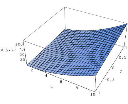
The scale factor on the full space-time, $a(y,t)$, is plotted in figure 2 for the special case $I=0$ and $\alpha=2$ or $n=-1$. Note that for $y=0$, equations (51) and (52) reduce to (42) and $n(0,t)=1$ respectively. There appears coordinate singularities on the space-like hypercone $y=\pm(\frac{t/t_{0}}{\alpha-1})$. This is presumably a consequence of the fact that the orthogonal geodesics emerging from the brane (which we used to set up our Gaussian normal system, $b^{2}=1$) do not cover the full five-dimensional space-time.

Figure 2: Behavior of $a(y,t)$ as a function of $t$ and $y$ for $n=-1$.

5 Brane Friedman equations with ${\cal L}(R)$

In this section we derive the Friedman equations for the brane metric in the presence of ${\cal L}(R)$ in the brane part of DGP action. Thus, for $I=0$ in equation (36) and using equation (23) we can write

$$\left[\dot{a}^{2}(0,t)-a^{\prime 2}(y,t)\right]a^{2}(y,t)=0.$$ (53)

Note that we assume $k=0$ and the bulk cosmological constant is zero. Taking the symmetry $y\leftrightarrow-y$ $(I^{+}=I^{-})$ for simplicity, equation (26) can be used to compute $a^{\prime}(y,t)$ on the two sides of the brane. We have in this case $[a^{\prime}(y,t)]=2a^{\prime}(0^{+},t)$. By continuity when $y\rightarrow 0$, equation (53) yields the generalized (first) Friedman equation

$$H^{2}-2\epsilon\frac{2\mu^{2}}{\kappa^{2}{\cal L}^{\prime}(R)}H=\frac{\mu^{2}}{3}\rho^{({\it tot})},$$ (54)

where the Hubble parameter is $H=\frac{\dot{a}(0,t)}{a(0,t)n(0,t)}$, $\kappa^{2}=m^{-3}_{5}$, $\mu^{2}=m^{-2}_{4}$ and $\epsilon=\pm 1$ is the sign of $[a^{\prime}(y,t)]$.

Now, let us discuss the solutions of the Friedman equation (54) together with (17) when the bulk cosmological constant vanishes. It is now apparent from (54) that the standard cosmology, namely the usual $4D$ Friedman equation (43) is recovered whenever the last term on the left hand side of (54) is subdominant with respect to the first term, namely when

$$H\gg 2\frac{\mu^{2}}{\kappa^{2}{\cal L}^{\prime}(R)}.$$ (55)

Thus using ansatzs (41) and (42), the above equation in terms of the Hubble radius $H^{-1}$ can be written

$$H^{-1}\ll(r_{c}n{\cal L}_{0})^{\frac{1}{2n-1}}(12-6/\alpha)^{\frac{n-1}{2n-1}},$$ (56)

where $r_{c}=\frac{m^{2}_{4}}{2m^{3}_{5}}$. For $n=1$ this matches the scale $r_{c}$ found in [10], setting the crossover between the $4D$ and $5D$ gravity regimes. For the special case $n=-1$, or $\alpha=2$ for which a power-law acceleration consistent with $t^{2}$ is obtained we have

$$H^{-1}\ll(81)^{\frac{1}{3}}(-r_{c}{\cal L}_{0})^{\frac{-1}{3}}.$$ (57)

Also, for $n\rightarrow 2$ $(\alpha\rightarrow\infty)$ one has

$$H^{-1}\ll(24r_{c}{\cal L}_{0})^{\frac{1}{3}}.$$ (58)

Thus, the Hubble radius $H^{-1}$ in this model depends on $n$. For the Hubble radius when equation (55) is not satisfied, there are two distinct behaviors depending on $\epsilon$. Equation (54) can indeed be rewritten as

$$H=\epsilon\frac{\mu^{2}}{\kappa^{2}{\cal L}^{\prime}(R)}\pm\sqrt{\frac{\mu^{2}}{3}\rho^{({\it tot})}+\frac{\mu^{4}}{\kappa^{4}{\cal L}^{\prime}(R)^{2}}}.$$ (59)

Let us start by examining the case where $\epsilon=-1$. Using condition $H{\cal L}^{\prime}(R)\ll r^{-1}_{c}$, one may then expand (54) to obtain

$$\frac{H}{{\cal L}^{\prime}(R)}=\frac{\kappa^{2}}{6}\rho^{({\it tot})},$$ (60)

or

$$H^{2}{\cal L}^{\prime}(R)^{-2}=\frac{\kappa^{4}}{36}\rho^{({\it tot})^{2}},$$ (61)

which is the full $5D$ regime with ${\cal L}(R)$ gravity on the brane. Equation (61) for $R^{n}$ becomes

$$H^{-4n+6}=\frac{\kappa^{4}}{36}(n{\cal L}_{0})^{2}\left(12-\frac{6}{\alpha}\right)^{2n-2}\left(\hat{\rho}+\rho^{({\it curv})}\right)^{2}.$$ (62)

Note that $\rho^{({\it curv})}$ is a function of $R$. One has thus a transition from a $4D$ to a $5D$ regime. If $\epsilon=1$, however, $H$ is always larger than $H_{\rm self}$ given by

$$\tilde{H}_{\rm self}=\frac{2\mu^{2}}{\kappa^{2}},$$ (63)

where $\tilde{H}_{\rm self}=H{\cal L}^{\prime}(R)$. For $R^{n}$ we find

$$H_{\rm self}=\left(\frac{2\mu^{2}}{\kappa^{2}n{\cal L}_{0}}\right)^{\frac{1}{2n-1}}(12-6/\alpha)^{\frac{1-n}{2n-1}},$$ (64)

and the expansion will never enter into a fully $5D$ regime. Thus for $k=0$ or $k=-1$ the Hubbel parameter is bounded from below by equation (64) for $R^{n}$ on the brane.

An interesting feature of the normal DGP models is the existence of ghost-like excitations [31, 32, 33]. It would therefore be interesting to briefly mention recent results relevant to the present work. In [33], the author has shown, in the context of normal DGP models, that if we introduce a positive cosmological constant on the brane $(Hr_{c}>1)$, then the spin-2 graviton will have a mass in the range $0<m^{2}<2H^{2}$ and that there is a normalizable brane fluctuation mode with mass $m^{2}=2H^{2}$. Although the brane fluctuation mode is healthy, the spin-2 graviton has a helicity-0 excitation which is known as a ghost. If we allow a negative cosmological constant on the brane, the brane bending mode becomes a ghost for $1/2<Hr_{c}<1$. This confirms the results obtained by the boundary effective action that there exists a scalar ghost mode for $Hr_{c}>1/2$. In a self-accelerating universe$Hr_{c}=1$, the spin-2 graviton has mass $m^{2}=2H^{2}$, which is known to be a special case for massive gravitons in de Sitter spacetime where the graviton has no helicity-0 excitation and so no ghost. However, in DGP models, there exists a brane fluctuation mode with the same mass and there arises a mixing between the brane fluctuation mode and the spin-2 graviton. Thus, according to this scenario, our model may be prone to having ghosts and this could be the subject of a separate investigation.

6 Conclusions

Brane models generally provide an interesting extension of our parameter space for gravitational theories. In this work we have discussed the DGP model with an arbitrary function of the Ricci scalar in the brane part of action. The cosmological evolution of this model was studied by solving the relevant dynamical equations. The components of the metric on the space-time was obtained for the $R^{n}$ term in $4D$ gravity. The evolution of the universe in such a scenario was shown to be consistent with the present observations, predicting an accelerated expansion. Finally we have shown that there exists two classes of solutions, close to the usual FRW cosmology for small enough Hubble radii for ${\cal L}(R)$ gravity.

References

• [1] N. Arkani-Hamed, S. Dimopoulos, G. Dvali, Phys. Lett. B 429 (1998) 263, [hep-ph/9803315],
N. Arkani-Hamed, S. Dimopoulos, G. Dvali, Phys. Rev. D 59 (1999) 086004, [hep-th/9807344].
• [2] I. Antoniadis, N. Arkani-Hamed, S. Dimopoulos, G. Dvali, Phys. Lett. B 436 (1998) 257, [hep-ph/9804398].
• [3] L. Randall, R. Sundrum, Phys. Rev. Lett. 83 (1999) 4690, [hep-th/0906064].
• [4] W. Mück, K. S. Viswanathan, I. V. Volovich, Phys. Rev. D 62 (2000) 105019, [hep-th/0004017].
• [5] R. Gregory, V. A. Rubakov, S. M. Sibiryakov, Class. Quan. Grav. 17 (2000) 4437, [hep-th/0003109].
• [6] I. Ya. Aref’eva, M. G. Ivanov, W. Mück, K. S. Viswanathan, I. V.Volovich, Nucl. Phys. B 590 (2000) 273, [hep-th/0004114].
• [7] M. Cveticˇˇ𝑐\check{c}, M. J. Duff, J.T. Liu, H. Lu, C. N. Pope, K. S. Stelle, Nucl. Phys. B 605 (2001) 141, [peh-th/0011167].
• [8] B. Abdesselam, N. Mohammedi, Phys. Rev. D 65 (2002) 084018, [hep-th/0110143].
• [9] E. A. Mirabelli, M. Perelstein, M. E. Peskin, Phys. Rev. Lett. 82 (1999) 2236, [hep-ph/981133],
T. Appelquist, H. C. Cheng, B. A. Dobrescu, Phys. Rev. D 64 (2001) 035002, [hep-ph/0201131],
T. G. Rizzo, Phys. Rev. D 64 (2001) 095010, [hep-ph/0106336],
S. Cullen, M. Perelstein, Phys. Rev. Lett. 83 (1999) 268, [hep-ph/9903422],
V. Barger, T. Han, C. Kao, R. J. Zhang, Phys. Lett. B 461 (1999) 34, [hep-ph/9905474],
S. Cassisi, V. Castellani, S. Degl’Innocenti, G. Fiorentini, B. Ricci, Phys. Lett. B 481 (2000) 323, [astro-ph/0002182],
M. Biesiada, B. Malec, Phys. Rev. D 65 (2002) 043008, [astro-ph/0109545],
S. Hannestad, G. G. Raffelt, Phys. Rev. Lett. 88 (2002) 071301, [hep-ph/0110067].
• [10] G. Dvali, G. Gabadadze, M. Porrati, Phys. Lett. B 485 (2000) 208, [hep-th/0005016].
• [11] G. Dvali, G. Gabadadze, Phys. Rev. D 63 (2001) 065007, [hep-th/0008054],
G. Dvali, G. Gabadadze, M. Kolanovic´´𝑐\acute{c}, F. Nitti, Phys. Rev. D 65 (2002) 024031, [hep-th/0106058].
• [12] R. Dick, Class. Quant. Grav. 18 (2001) R1, [hep-th/0105320].
• [13] R. Dick, Actaphys. Polon. B 32 (2001) 3669, [hep-th/0110162].
• [14] R. Cordero, A. Vilenkin, Phys. Rev. D 65 (2002) 083519, [hep-th/0107175].
• [15] A. Lue, Phys. Rept. 423 (2006) 1, [astro-ph/0510068].
• [16] A. G. Riess et. al. [Supernova Search Team Collaboration], Astron. J. 116 (1998) 1006, [astro-ph/9805201].
• [17] S. Perlmutter et. al., Astron. J. 517 (1999) 565, [astro-ph/9812133],
D. N. Spergel et. al., Astrophys. J. Suppl. 148 (2003) 175, [astro-ph/0302209].
• [18] C. L. Bennett et. al., Astrophys. J. Suppl. 148 (2003) 1, [astro-ph/0302207].
• [19] C. B. Netterfiled et. al., Astrophys. J. 571 (2002) 604, [astro-ph/0104460],
N. W. Halverson et. al., Astrophys. J. 568 (2002) 38, [astro-ph/0104489].
• [20] S. M. Carroll, Living Rev. Rel. 4 (2001) 1, [astro-ph/0004075].
• [21] C. Deffayet, Phys. Lett. B 502 (2001) 199, [hep-th/0010186],
C. Deffayet, G. R. Dvali and G. Gabadadze, Phys. Rev. D 65 (2002) 044023, [astro-ph/0105068],
C. Deffayet and S. J. Landau, J. Raux, M. Zaldarriaga and P. Astier, Phys. Rev. D 66 (2002) 024019, [astro-ph/0201164],
J. S. Alcaniz, Phys. Rev. D 65 (2002) 123514, [astro-ph/0202492],
D. Jain, A. Dev and J. S. Alcaniz, Phys. Rev. D 66 (2002) 083511, [astro-ph/0206224],
A. Lue, R. Scoccimarro, G. Starkman, Phys. Rev. D 69 (2004) 044005, [astro-ph/0307034].
• [22] S. Capozziello, Int. J. Mod. Phys. D 11 (2002) 483, [astro-ph/0201033],
S. Capozziello, Int. J. Mod. Phys. D 12 (2003) 1969, [astro-ph/0307018].
• [23] S. M. Carroll, V. Duvvuri, M. Trodden, M. Turner, Phys. Rev. D 70 (2004) 043528, [astro-ph/0306438].
• [24] K. Atazadeh and H. R. Sepangi, Phys. Lett. B 643 (2006) 76, [gr-qc/0610107].
• [25] K. Nozari, Phys. Lett. B 652 (2007) 159, [hep-th/0707.0719],
K. Nozari, JCAP 09 (2007) 003, [hep-th/0708.1611].
• [26] P. Bine´´𝑒\acute{e}truy, C. Deffayet, D. Langlois, Nucl. Phys. B 565 (2000) 269, [hep-th/9905012].
• [27] P. Bine´´𝑒\acute{e}truy, C. Deffayet, U. Ellwanger, D. Langlois, Phys. Lett. B 477 (2000) 285, [hep-th/9910219].
• [28] P. P. Avelino, C. J. A. P. Martins, Astrophys.J. 565 (2002) 661, [astro-ph/0106274].
• [29] C. Deffayet, G. Dvali, G. Gabadadze, [astro-ph/0106449].
• [30] T. Padmanabhan, Phys. Rept. 380 (2003) 235, [hep-th/ 0212290].
• [31] M. A. Luty, M. Porrati and R. Rattazzi, JHEP 0309 (2003) 029, [hep-th/ 0303116].
• [32] A. Nicolis and R. Rattazzi, JHEP 0406 (2004) 059, [hep-th/0404159].
• [33] K. Koyama, Phys.Rev. D 72 (2005) 123511, [hep-th/0503191].