Transverse and longitudinal momentum spectra of fermions
produced in strong SU(2) fields

Abstract

We study the transverse and longitudinal momentum spectra of fermions produced in a strong, time-dependent non-Abelian SU(2) field. Different time-dependent field strengths are introduced. The momentum spectra are calculated for the produced fermion pairs in a kinetic model. The obtained spectra are similar to the Abelian case, and they display exponential or polynomial behaviour at high $p_{T}$, depending on the given time dependence. We investigated different color initial conditions and discuss the recognized scaling properties for both Abelian and SU(2) cases.

I Introduction

During last years large amount of data on particle spectra have been collected in relativistic heavy ion collisions at the Super-Proton Synchrotron (SPS, CERN) and at the Relativistic Heavy Ion Collider (RHIC, BNL) at c.m. energy of $\sqrt{s}=10-200$ GeV QM04 ; QM05 in a wide transverse momentum range, $0\leq p_{T}\leq 20$ GeV. Since the microscopic mechanisms of hadron production in hadron-hadron and heavy ion collisions are not fully understood, thus it is very important to improve our theoretical understanding on this field. The forthcoming hadron and heavy ion experiments at the Large Hadron Collider (LHC, CERN) at $\sqrt{s}=5500$ GeV will increase the transverse momentum window to $0\leq p_{T}\leq 50$ GeV. Thus LHC experiments will become a decisive test between different perturbative and non-perturbative models of hadron formation, especially in the high-$p_{T}$ region.

Theoretical descriptions of particle production in high energy $pp$ collisions are based on the introduction of chromoelectric flux tube (’string’) models, where these tubes are connecting the quark and diquark constituents of the colliding protons FRITIOF ; HIJ ; RQMD ; Topor0507 . String picture is a good example of how to convert the kinetic energy of a collision into field energy. New hadrons will be produced via quark-antiquark and diquark-antidiquark pair production from the field energy, namely from the unstable flux tubes. These models can describe experimental data very successfully at small $p_{T}$, especially at $p_{T}<2-3$ GeV. At higher $p_{T}$ one can apply perturbative QCD-based models FieldFeyn ; Wang00 ; Yi02 , which can provide the necessary precision to analyse nuclear effects in the nuclear collisions.

However, at RHIC and LHC energies the string density is expected to be so large that a strong collective gluon field will be formed in the whole available transverse volume. Furthermore, the gluon number will be so high that a classical gluon field as the expectation value of the quantum field can be considered and investigated in the reaction volume. The properties of such non-Abelian classical fields and details of gluon production were studied very intensively during the last years, especially asymptotic solutions (for summaries see Refs. McL02 ; IanVen03 ). Fermion production was calculated recently Gelis04 ; Blaiz04 . Lattice calculations were performed to describe strong classical fields under finite space-time conditions in the very early stage of heavy ion collision, especially immediately after the overlap Krasnitz ; Lappi ; Lappi_more . New methods have been developed to investigate the influence of inhomogeneity on particle production Gies05 ; Dunne05 ; Kim06 .

Fermion pair production together with boson pair production were investigated by different kinetic models of particle production from strong Abelian Gatoff87 ; Kluger91 ; Gatoff92 ; Wong95 ; Eisenberg95 ; Vin02 ; Per03 ; Per06 and non-Abelian Prozor03 ; Diet03 ; Nayak fields. These calculations concentrated mostly on the bulk properties of the gluon and quark matter, the time evolution of the system, the time dependence of energy and particle number densities, and the appearance of fast thermalization.

Our main interest is the transverse momentum distribution of produced fermions and bosons, however the longitudinal momentum can become equally interesting considering wide rapidity ranges. In our previous paper (see Ref. SkokLev05 ) we investigated the Abelian case, namely particle pair-production in a strong external electric field. We have focused on the numerical solution of a kinetic model and discussed the influence of the field strength applying different time dependences. We have demonstrated a scaling behaviour in time and transverse momenta, namely $t\cdot E_{0}^{1/2}$ and $k_{T}/E_{0}^{1/2}$. The kinetic equation and the numerical calculation yielded a fermion dominance in the mid-rapidity region. In case of realistic Bjorken type time evolution our numerical result on fermion spectra has overlapped the boson spectra obtained in 1+2 dimensional lattice calculations both in magnitude and shape.

In this paper we solve the kinetic model in the presence of an SU(2) non-Abelian color field. We focus on the determination of the appropriate kinetic equation system and its numerical solution in case of different initial conditions. Section 2 summarizes the kinetic equation for color Wigner function. In Section 3 we introduce phenomenologically the fermion distribution function. In Section 4 the kinetic equation and its simplifications are displayed in detail, especially with zero fermion mass. In Section 5 we present kinetic equation for the case, when external non-Abelian field have fixed direction in color space. The appropriate form of the kinetic equation is determined, which was solved numerically at different time-dependent strong fields. Results on field components and fermion distribution functions are displayed in Section 6. We display recognized scaling properties of the solutions in Section 7. In Appendix A we show a special non-Abelian setup, which leads to the similar results obtained in the Abelian case.

II The kinetic equation for the Wigner function

The fermion production in a strong external field can be characterized by a space homogeneous Wigner function, $W(\mathbf{k};t)$. The evolution of this Wigner function is investigated by the kinetic equation in the frame of the covariant single-time formalism, where a time-dependent Abelian ($A^{\mu}$) BialBirul91 ; Heinz96 ; Heinz98 ; Holl02 or non-Abelian ($A_{\mu}^{a}$) Heinz98 ; Prozor03 external field is included. Here we choose a longitudinally dominant color vector field in Hamilton gauge described by the 4-potential

$$A_{\mu}^{a}=(0,-{\bf{A}}^{a})=(0,0,0,A_{3}^{a})\ .$$ (1)

The Wigner function depends on the 3-momenta $\mathbf{k}=(k_{1},k_{2},k_{3})$. In the ”instant” frame of reference Prozor03 we obtain the kinetic equation for $W(\mathbf{k};t)$ as

$$\partial_{t}W+\frac{g}{8}\frac{\partial}{\partial k_{i}}\left(4\{W,F_{0i}\}+\right.$$

$$\ \ \ \ \ \ \ \left.+2\left\{F_{i\nu},[W,\gamma^{0}\gamma^{\nu}]\right\}-\left[F_{i\nu},\{W,\gamma^{0}\gamma^{\nu}\}\right]\right)=$$

$$=ik_{i}\{\gamma^{0}\gamma^{i},W\}-im[\gamma^{0},W]+ig\left[A_{i}\,,[\gamma^{0}\gamma^{i},W]\right].\ \ \$$ (2)

Here $m$ denotes the current mass of the fermion produced in the strong field and $g$ is the coupling constant.

The color decomposition with $SU(N_{c})$ generators in fundamental representation ($t^{a}$) is

$$W=W^{s}+W^{a}t^{a},\,\,\ \ \ a=1,2,...,N_{c}^{2}-1\ ,$$ (3)

where $W^{s}$ is the color singlet and $W^{a}$ is the color multiplet component (triplet in $SU(2)$ with $N_{c}=2$).

The spinor decomposition is the following:

$$W^{s|a}=a^{s|a}+b^{s|a}_{\mu}\gamma^{\mu}+c^{s|a}_{\mu\nu}\sigma^{\mu\nu}+d^{s|a}_{\mu}\gamma^{\mu}\gamma^{5}+ie^{s|a}\gamma^{5}.$$ (4)

The time evolution of the Wigner function is described by eq. (2). Using the color and spinor decomposition terms in eqs.(3)-(4), we will determine the time evolution numerically. However, our main goal is to obtain the transverse momentum spectra of the produced fermion pairs, thus we need to introduce the fermion distribution function. There is no straightforward way to define this distribution function, but we can find a phenomenological way, summarized in the next chapter.

III The fermion distribution function from the energy density

The energy density carried by the produced fermions is defined throughout the Wigner function Heinz98 ; Prozor03 :

$$\varepsilon_{f}=\mbox{Tr}\langle\,(m-\gamma^{i}k_{i})W+\omega(\mathbf{k})\,\rangle\ ,$$ (5)

where the second term fixes the zero energy level to the physical value (note, that expression (5) is free from divergent vacuum contribution). Here the one particle energy is denoted by $\omega(\mathbf{k})=\sqrt{\mathbf{k}^{2}+m^{2}}$. The trace is over color and spinor and the averaging is taken over momenta:

$$\langle\,{\cal X}\,\rangle=\int\frac{d^{3}k}{(2\pi)^{3}}{\cal X}(\mathbf{k};t).$$ (6)

After the color and spinor decomposition one obtains

$$\varepsilon_{f}=2N_{c}\langle\,2ma^{s}+2\mathbf{k}\,\mathbf{b}^{s}+\omega(\mathbf{k})\,\rangle.$$ (7)

In parallel, focusing on one-particle distribution function the usual energy density formula has the following form:

$$\varepsilon_{f}=4N_{c}\langle\,\omega(\mathbf{k})f_{f}(\mathbf{k})\,\rangle=4N_{c}\int\frac{d^{3}k}{(2\pi)^{3}}\omega(\mathbf{k})f_{f}(\mathbf{k}).$$ (8)

Note, that both averages (5) and (8) may contain ultraviolet divergence, that can be properly regularized (for Abelian fields see e.g. Cooper:1992hw ; grib ). However, since we are not going to calculate bulk properties of produced pairs, the issue of regularization is not important in current consideration and will be considered elsewhere.

Now, combining eq.(7) and eq.(8) one can derive phenomenologically a distribution function, namely

$$f_{f}(\mathbf{k},t)=\frac{ma^{s}(\mathbf{k},t)+\mathbf{k}\,\mathbf{b}^{s}(\mathbf{k},t)}{\omega(\mathbf{k})}+\frac{1}{2}\ .$$ (9)

The time dependence in $f_{f}(\mathbf{k},t)$ is connected to the time-evolution of $a^{s}(\mathbf{k},t)$ and $\mathbf{b}^{s}(\mathbf{k},t)$, which is followed by solving the decomposed kinetic equation of eq. (2).

The fermion distribution function should be zero in vacuum. The expression in eq. (9) satisfies this request. Indeed the vacuum solution ($A_{\mu}=0$) for the singlet Wigner function has the following form (see Ref. Prozor03 )

$$W^{s}=-\frac{1}{2}\frac{m+\mathbf{k}\mathbf{\gamma}}{\omega(\mathbf{k})}\ .$$ (10)

The vacuum solution for the multiplet Wigner function is zero, $W^{a}=0$. The substitution of this Wigner function into the definition of the distribution function in eq.(9) leads to $f_{f}=0$ in vacuum, which is physically correct. Furthermore, one can see that $f_{f}(\mathbf{k},t)$ is positive definite in presence of a non-zero field ($A_{\mu}\neq 0$).

Although our fermion distribution function $f_{f}(\mathbf{k},t)$ has been postulated phenomenologically and possibly it is not a unique solution, but it seems to be the right tool to investigate the time evolution of the energy distribution at the microscopical level in a space homogeneous environment.

IV Kinetic equation for the Wigner function in SU(2)

Our basic aim is to determine the fermionic distribution function and its time evolution in the presence of a strong, time-dependent non-Abelian SU(2) field. For this task we need to substitute the color and spinor decomposed Wigner function of eq. (3) into the kinetic equation in eq. (2). After evaluating the color and spinor indeces we obtain a system of coupled differential equations, which consists of 32 components in SU(2):

$$\partial_{t}a^{s}+\frac{g}{4}E^{a}\frac{\partial}{\partial k_{3}}a^{a} = -4\mathbf{k}\mathbf{c}_{1}^{s},\,$$ (11)

$$\partial_{t}a^{a}+gE^{a}\frac{\partial}{\partial k_{3}}a^{s} = -4\mathbf{k}\mathbf{c}_{1}^{a},\,$$ (12)

$$\partial_{t}b^{s}_{0}+\frac{g}{4}E^{a}\frac{\partial}{\partial k_{3}}b^{a}_{0} = 0,$$ (13)

$$\partial_{t}b^{a}_{0}+gE^{a}\frac{\partial}{\partial k_{3}}b^{s}_{0} = 2gf^{abc}\mathbf{A}^{b}\mathbf{b}^{c},\,$$ (14)

$$\partial_{t}\mathbf{b}^{s}+\frac{g}{4}E^{a}\frac{\partial}{\partial k_{3}}\mathbf{b}^{a} = 2\mathbf{k}\times\mathbf{d}^{s}+4m\mathbf{c}^{s}_{1},\,$$ (15)

$$\partial_{t}\mathbf{b}^{a}+gE^{a}\frac{\partial}{\partial k_{3}}\mathbf{b}^{s} = 2\mathbf{k}\times\mathbf{d}^{a}+4m\mathbf{c}^{a}_{1}+$$ (16)

$$+2gf^{abc}\mathbf{A}^{b}b_{0}^{c},\,$$

$$\partial_{t}\mathbf{c}_{1}^{s}+\frac{g}{4}E^{a}\frac{\partial}{\partial k_{3}}\mathbf{c}_{1}^{a} = \mathbf{k}a^{s}-m\mathbf{b}^{s},\,$$ (17)

$$\partial_{t}\mathbf{c}_{1}^{a}+gE^{a}\frac{\partial}{\partial k_{3}}\mathbf{c}_{1}^{s} = \mathbf{k}a^{a}-m\mathbf{b}^{a}+$$ (18)

$$-2gf^{abc}(\mathbf{A}^{b}\times\mathbf{c}_{2}^{c}),\,$$

$$\partial_{t}\mathbf{c}_{2}^{s}+\frac{g}{4}E^{a}\frac{\partial}{\partial k_{3}}\mathbf{c}_{2}^{a} = \mathbf{k}e^{s},\,$$ (19)

$$\partial_{t}\mathbf{c}_{2}^{a}+gE^{a}\frac{\partial}{\partial k_{3}}\mathbf{c}_{2}^{s} = \mathbf{k}e^{a}-2gf^{abc}(\mathbf{A}^{b}\times\mathbf{c}_{1}^{c}),\,$$ (20)

$$\partial_{t}d^{s}_{0}+\frac{g}{4}E^{a}\frac{\partial}{\partial k_{3}}d^{a}_{0} = 2me^{s},$$ (21)

$$\partial_{t}d^{a}_{0}+gE^{a}\frac{\partial}{\partial k_{3}}d^{s}_{0} = 2me^{s}+2gf^{abc}\mathbf{A}^{b}\mathbf{d}^{c}\,,$$ (22)

$$\partial_{t}\mathbf{d}^{s}+\frac{g}{4}E^{a}\frac{\partial}{\partial k_{3}}\mathbf{d}^{a} = 2\mathbf{k}\times\mathbf{b}^{s},\,$$ (23)

$$\partial_{t}\mathbf{d}^{a}+gE^{a}\frac{\partial}{\partial k_{3}}\mathbf{d}^{s} = 2\mathbf{k}\times\mathbf{b}^{a}+2gf^{abc}\mathbf{A}^{b}d_{0}^{c},\,$$ (24)

$$\partial_{t}e^{s}+\frac{g}{4}E^{a}\frac{\partial}{\partial k_{3}}e^{a} = -4\mathbf{k}\mathbf{c}_{2}^{s}-2md_{0}^{s},\,$$ (25)

$$\partial_{t}e^{a}+\frac{g}{4}E^{a}\frac{\partial}{\partial k_{3}}e^{s} = -4\mathbf{k}\mathbf{c}_{2}^{a}-2md_{0}^{a}.$$ (26)

Here we use the notation $b^{s|a}_{\mu}=(b^{s|a}_{0},-\mathbf{b}^{s|a})$, and a similar one for $d^{s|a}_{\mu}$. The antisymmetric tensor component of the Wigner function is defined as $c^{\mu\nu}=(\mathbf{c}_{1},\mathbf{c}_{2})$ Landau2 . The strength of the color electric field is $E^{a}\equiv E^{a}_{3}=-\dot{A}_{3}^{a}$.

Since the mass of light quarks is small, we neglect the mass term in our SU(2) calculation. In this case the distribution function for massless fermions is solely defined by $\mathbf{b}^{s}$:

$$f_{f}(\mathbf{k},t)=\frac{\mathbf{k}\,\mathbf{b}^{s}}{|\mathbf{k}|}+\frac{1}{2}\ ,$$ (27)

The zero fermion mass leads to the simplification of the above kinetic equation, which finally is splitted into two independent parts: one for $a^{s|a},\mathbf{c}_{1}^{s|a},\mathbf{c}_{2}^{s|a},e^{s|a}$ and another one for $b_{0}^{s|a},\mathbf{b}^{s|a},d_{0}^{s|a},\mathbf{d}^{s|a}$. One can recognize that the second set completely defines the evolution of the fermion distribution function. This way the chiral symmetry of the massless case is manifested itself. Thus we focus on these equations, only:

$$\partial_{t}\mathbf{b}^{s}+\frac{g}{4}E^{a}\frac{\partial}{\partial k_{3}}\mathbf{b}^{a} = 2\mathbf{k}\times\mathbf{d}^{s},\,$$ (28)

$$\partial_{t}\mathbf{b}^{a}+gE^{a}\frac{\partial}{\partial k_{3}}\mathbf{b}^{s} = 2\mathbf{k}\times\mathbf{d}^{a}+2gf^{abc}\mathbf{A}^{b}b_{0}^{c},\,$$ (29)

$$\partial_{t}\mathbf{d}^{s}+\frac{g}{4}E^{a}\frac{\partial}{\partial k_{3}}\mathbf{d}^{a} = 2\mathbf{k}\times\mathbf{b}^{s},\,$$ (30)

$$\partial_{t}\mathbf{d}^{a}+gE^{a}\frac{\partial}{\partial k_{3}}\mathbf{d}^{s} = 2\mathbf{k}\times\mathbf{b}^{a}+2gf^{abc}\mathbf{A}^{b}d_{0}^{c},\,$$ (31)

$$\partial_{t}b^{s}_{0}+\frac{g}{4}E^{a}\frac{\partial}{\partial k_{3}}b^{a}_{0} = 0,$$ (32)

$$\partial_{t}b^{a}_{0}+gE^{a}\frac{\partial}{\partial k_{3}}b^{s}_{0} = 2gf^{abc}\mathbf{A}^{b}\mathbf{b}^{c},\,$$ (33)

$$\partial_{t}d^{s}_{0}+\frac{g}{4}E^{a}\frac{\partial}{\partial k_{3}}d^{a}_{0} = 0,$$ (34)

$$\partial_{t}d^{a}_{0}+gE^{a}\frac{\partial}{\partial k_{3}}d^{s}_{0} = 2gf^{abc}\mathbf{A}^{b}\mathbf{d}^{c}.$$ (35)

The vacuum initial conditions are given by eq.(10):

$$\mathbf{b}^{s}(t\to-\infty)=-\frac{\mathbf{k}}{2|\mathbf{k}|},$$ (36)

The other components of the Wigner function have zero initial values.

The system of equations in (28)-(35) can be solved numerically for different color configurations. Thus the evolution of the color could be followed in detail, similarly to the color evolution in the Wong Yang-Mills equations WongYM ; Colorequi . However, in the next section for the sake of simplicity we will consider assumption that the external field has a fixed direction in color space.

V Kinetic equation in SU(2) with external field of fixed direction in color space

The equations (28)-(35) provides a full description of the fermion production in a time-dependent SU(2) color field. Here we will consider the case of the external field, that has a fixed direction in color space: $\mathbf{A}^{a}\equiv\mathbf{A}^{\diamond}n^{a}$, where $n^{a}n^{a}=1$ and $\partial_{t}n^{a}=0$, in general case, and $A_{3}^{a}\equiv A^{\diamond}n^{a}$, $a=1,2,3$ in our calculation. Then the equations (28)-(35) have the following particular solution:

$$\mathbf{b}^{a}=\mathbf{b}^{\diamond}n^{a},\,\,\mathbf{d}^{a}=\mathbf{d}^{\diamond}n^{a}.$$ (37)

Taking into account the zero initial conditions for $b_{0}^{a},d_{0}^{a}$ and $b_{0}^{s},d_{0}^{s}$, the equations (32)-(35) become trivial and do not contribute to the set of equations (28-31), the last simplifies to give

$$\partial_{t}\mathbf{b}^{s}+\frac{3g}{4}E^{\diamond}\frac{\partial}{\partial k_{3}}\mathbf{b}^{\diamond} = 2\mathbf{k}\times\mathbf{d}^{s},\,$$ (38)

$$\partial_{t}\mathbf{b}^{\diamond}+gE^{\diamond}\frac{\partial}{\partial k_{3}}\mathbf{b}^{s} = 2\mathbf{k}\times\mathbf{d}^{\diamond},\,$$ (39)

$$\partial_{t}\mathbf{d}^{s}+\frac{3g}{4}E^{\diamond}\frac{\partial}{\partial k_{3}}\mathbf{d}^{\diamond} = 2\mathbf{k}\times\mathbf{b}^{s},\,$$ (40)

$$\partial_{t}\mathbf{d}^{\diamond}+gE^{\diamond}\frac{\partial}{\partial k_{3}}\mathbf{d}^{s} = 2\mathbf{k}\times\mathbf{b}^{\diamond}.$$ (41)

Introducing the unit vector collinear to the field direction, $\mathbf{n}=\mathbf{E}^{\diamond}/|\mathbf{E}^{\diamond}|=(0,0,1)$, and $\mathbf{k}_{\perp}=(k_{1},k_{2},0)$, we can perform the following vector decomposition:

$$\mathbf{b}^{\diamond|s} = b_{3}^{\diamond|s}\mathbf{n}+b_{\perp}^{\diamond|s}\frac{\mathbf{k}_{\perp}}{k_{\perp}},$$ (42)

$$\mathbf{d}^{\diamond|s} = d^{\diamond|s}\mathbf{n}\times\frac{\mathbf{k}_{\perp}}{k_{\perp}}\ .$$ (43)

Finally we obtain 6 equations, only:

$$\partial_{t}b^{s}_{\perp}+\frac{3g}{4}E^{\diamond}\frac{\partial}{\partial k_{3}}b_{\perp}^{\diamond} = -2k_{3}d^{s}\ ,$$ (44)

$$\partial_{t}b^{s}_{3}+\frac{3g}{4}E^{\diamond}\frac{\partial}{\partial k_{3}}b_{3}^{\diamond} = 2k_{\perp}d^{s},$$ (45)

$$\partial_{t}d^{s}+\frac{3g}{4}E^{\diamond}\frac{\partial}{\partial k_{3}}d^{\diamond} = 2k_{3}b_{\perp}^{s}-2k_{\perp}b_{3}^{s},$$ (46)

$$\partial_{t}b_{\perp}^{\diamond}+gE^{\diamond}\frac{\partial}{\partial k_{3}}b^{s}_{\perp} = -2k_{3}d^{\diamond},$$ (47)

$$\partial_{t}b_{3}^{\diamond}+gE^{\diamond}\frac{\partial}{\partial k_{3}}b^{s}_{3} = 2k_{\perp}d^{\diamond},$$ (48)

$$\partial_{t}d^{\diamond}+gE^{\diamond}\frac{\partial}{\partial k_{3}}d^{s} = 2k_{3}b_{\perp}^{\diamond}-2k_{\perp}b_{3}^{\diamond}.$$ (49)

These equations determine the time evolution of the wanted distribution function:

$$f_{f}(\mathbf{k},t)=\frac{k_{3}\,{b}^{s}_{3}+k_{\perp}\,b^{s}_{\perp}}{|\mathbf{k}|}+\frac{1}{2}\ .$$ (50)

The numerical solution of eqs. (44)-(49) requires initial conditions. In our case the appropriate vacuum initial conditions are the following:

$$b^{s}_{3}(\mathbf{k},t=-\infty) = -\frac{k_{3}}{2k}\ ,$$ (51)

$$b^{s}_{\perp}(\mathbf{k},t=-\infty) = -\frac{k_{\perp}}{2k}\ ,$$ (52)

$$b_{3}^{\diamond}(\mathbf{k},t=-\infty) = b_{\perp}^{\diamond}(\mathbf{k},t=-\infty)=0\ ,$$ (53)

$$d^{\diamond}(\mathbf{k},t=-\infty) = d^{s}(\mathbf{k},t=-\infty)=0.$$ (54)

Now we have all parts to proceed numerically for any time-dependent field strength and determine the momentum distribution of the produced fermions.

VI Numerical results

In heavy ion collisions, one can assume three different types of time dependence for the color field to be formed: a) pulse-like field develops with a fast increase, which is followed by a fast fall in the field strength; b) formation of a constant field ($E_{0}$) is maintained after the fast increase in the initial time period; c) scaled decrease of the field strength appears, which is caused by particle production and/or transverse expansion, and the decrease is elongated in time much further than the pulse-like assumption.

Figure 1: The time dependence of external field $E(t)$ in three physical scenarios: a) pulse (dotted line); b) constant field, $E_{0}$ (dashed line); c) scaled decrease (solid line).

Figure  1 displays three sets for the time dependence of the external field SkokLev05 :

$$E_{pulse}^{\diamond}(t) =E_{0}\cdot\left[1-\textrm{tanh}^{2}(t/\delta)\right]\hskip 17.07182pt$$ (55)

$$E_{const}^{\diamond}(t) =\left\{\begin{array}[]{ll}E^{\diamond}_{pulse}(t)&{\textrm{a}t}\ \ {t<0}\\ E_{0}&{\textrm{a}t}\ \ {t\geq 0}\end{array}\right.$$ (58)

$$E_{scaled}^{\diamond}(t) =\left\{\begin{array}[]{ll}E^{\diamond}_{pulse}(t)&{\textrm{a}t}\ \ {t<0}\\ \frac{E_{0}}{(1+t/t_{0})^{\kappa}}&{\textrm{a}t}\ \ {t\geq 0}\end{array}\right.$$ (61)

In eq. (55) we choose $\delta=0.1/\,E_{0}^{1/2}$, which corresponds to RHIC energies. In eq. (61) the value $\kappa=2/3$ indicates a longitudinally scaled Bjorken expansion with $t_{0}=0.01/\,E_{0}^{1/2}$. In fact, the whole time dependence is scaled by ${E_{0}}^{1/2}$.

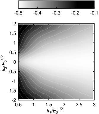
Figure 2: The momentum dependence of the transverse, color singlet component $b^{s}_{\perp}(k_{\perp},k_{3})$ at $t=2/E_{0}^{1/2}$ for the Bjorken expanding scenario.

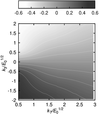
Figure 3: The momentum dependence of the longitudinal, color singlet component $b^{s}_{3}(k_{\perp},k_{3})$ at $t=2/E_{0}^{1/2}$ for the Bjorken expanding scenario.

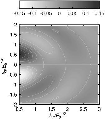
Figure 4: The momentum dependence of the transverse, color component $b^{\diamond}_{\perp}(k_{\perp},k_{3})$ at $t=2/E_{0}^{1/2}$ for the Bjorken expanding scenario.

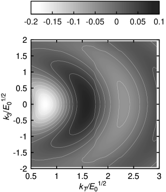
Figure 5: The momentum dependence of the longitudinal, color component $b^{\diamond}_{3}(k_{\perp},k_{3})$ at $t=2/E_{0}^{1/2}$ for the Bjorken expanding scenario.

Before comparing the momentum distributions obtained numerically in the three different physical scenarios of eqs.(55)-(61) we investigate our results on the quantities responsible for the momentum distribution. Detailed numerical results are shown in the following five figures for the specific case of the Bjorken expansion.

The distribution function $f_{f}(k_{\perp},k_{3})$ depends directly on $b^{s}_{\perp}(k_{\perp},k_{3})$ and $b^{s}_{3}(k_{\perp},k_{3})$ as eq. (50) shows. Figure 2 and 3 display the magnitudes of these quantities in 2-dimensional plots. The $k_{3}$-symmetry of $b^{s}_{\perp}(k_{\perp},k_{3})$ can be seen clearly, as well as the asymmetric behaviour of $b^{s}_{3}(k_{\perp},k_{3})$. The value of these functions are in ${\cal{O}}(1)$.

The distribution function $f_{f}(k_{\perp},k_{3})$ is color neutral, thus the color quantities $b^{\diamond}_{\perp}(k_{\perp},k_{3})$ and $b^{\diamond}_{3}(k_{\perp},k_{3})$ do not contribute directly. However, they play important role in the kinetic equation, see eqs. (44)-(49). Their oscillating behaviour can be seen on Figure 4 and 5.

Figure 6: Longitudinal momentum ($k_{3}$) spectra for fermions at $k_{\perp}/E_{0}^{1/2}=0.5$ and $t=2/E_{0}^{1/2}$ in the three physical scenarios (see Fig. 1 and text for explanation).

Figure 7: Longitudinal momentum ($k_{3}$) spectra for fermions at $k_{\perp}/E_{0}^{1/2}=2.5$ and $t=2/E_{0}^{1/2}$ in the three physical scenarios (see Fig. 1 and text for explanation).

Figure 8: Transverse momentum spectra for fermions at $k_{3}/E_{0}^{1/2}=0,1,2$ in the time step $t=2/E_{0}^{1/2}$ for the Bjorken expansion scenario.

Now we return to the three physical scenarios with different time dependence described in eqs. (55)-(61) and investigate the fermion spectra at a large time, $t=2/E_{0}^{1/2}$. Figure 6 indicates the behaviour of the longitudinal momentum spectra at small transverse momentum value, where we choose $k_{\perp}/E_{0}^{1/2}=0.5$. Pulse-type time dependence leads to a narrow $k_{3}$-distribution (dotted line), which mimics a Landau-type hydrodynamical initial condition. The longitudinal spectra from constant field scenario (dashed line) leads to a flat distribution function in $k_{3}$. This result agrees well with a 1-dimensional, longitudinally invariant hydrodynamical initial condition, as we expect. Considering the scaled field scenario (solid line), since its time dependence is very similar to the pulse-type case (see Fig. 1), then the similarity in the longitudinal spectra is well understandable.

If we increase the transverse momentum and choose $k_{\perp}/E_{0}^{1/2}=2.5$, then Figure 7 displays the obtained longitudinal spectra: the $k_{3}$ dependence becomes very similar in the small $k_{3}$ region for the three different time evolution. For pulse-type time dependence (dotted line) and for constant field scenario (dashed line) even the magnitude is very close to each other. Further numerical investigations are needed to understand this similarities.

The interplay between transverse and longitudinal momentum spectra is displayed on Figure 8. In the Bjorken expansion scenario of eq. (61) we choose different longitudinal momentum windows, namely $k_{3}/E_{0}^{1/2}=0,1,2$ and extract the transverse momentum spectra at $t=2/E_{0}^{1/2}$. On Figure 8 one can see large deviation at small transverse momenta and similar spectra at high transverse momenta: hard fermion production is similar at different rapidities, but soft production (and any ’effective temperature’) is very strongly rapidity dependent.

Figure 9 displays the transverse momentum spectra for the three different physical scenario at momentum $k_{3}=0$ and time $t=2/E_{0}^{1/2}$. Pulse-type time dependence leads to exponential spectra (dotted line), $f_{f}\propto\exp(k_{T}/T)$ with slope value $T=1.54\cdot E_{0}^{1/2}$. In the other two cases, we obtain non-exponential spectra generated by the long-lived field. Here the spectra from constant (dashed lines) and scaled (solid lines) fields are close, because the production and annihilation rates balance each other. Slight differences appear because of the fast fall of the scaled field immediately after $t=0$.

Figure 9: The transverse momentum spectra for fermions at $k_{3}=0$ and $t=2/E_{0}^{1/2}$ in the three physical scenarios (see Fig. 1 and text for explanation).

Figure 10: Transverse momentum spectra of fermions from our calculation with scaled time evolution, $E_{scaled}(t)$, for SU(2) case (solid line), and from Ref. SkokLev05 for U(1) (dash-dotted line).

Figure 11: The ratio of the numerical results from Figure 10 on transverse momentum spectra for fermions in a linear scale: the SU(2) case (this calculation) is divided by the U(1) case from Ref. SkokLev05 .

In our previous paper SkokLev05 we considered fermion production in U(1) classical field. Comparison between current SU(2) calculation and U(1) results can be made, if we fix both field strength at the same value. Taking the value $E_{0}^{1/2}/\Lambda_{s}=0.54$ used in Ref. SkokLev05 , we obtain transverse momentum spectra depicted in the Figure 10, where particle production in the scaled field scenario was considered. We have found that the obtained transverse distribution functions for fermions are close to each other and have at almost the same shape. Figure 11 displays the ratio of the two numerical results on a linear scale. It clearly shows the appearance of a numerical value of $f_{\rm SU(2)}(k_{\perp})/f_{\rm U(1)}(k_{\perp})=0.75$ for transverse momenta $k_{\perp}\geq\Lambda_{s}$. This value may indicate the presence of scaling solutions of the investigated kinetic equations. The direct study of the kinetic equations in Section IV and V does not reveal scaling, but special cases can indicate such a behaviour.

VII Scaling solutions

In this section we consider specific initial conditions and corresponding solution for the kinetic equations eqs. (44)-(49). At first we assume the singlet and the color multiplet components have the same initial values. This “symmetry” is generally violated by vacuum initial conditions demanding $b^{\diamond}$ and $d^{\diamond}$ to be zero in vacuum in contract to initial conditions for $b^{s}$ and $d^{s}$ (cf. (51)-(54)). Accepting this assumption, one may note that eqs. (44)-(49) have the following special solution: $b^{\diamond}=\eta b^{s}$ and $d^{\diamond}=\eta d^{s}$, where $\eta$ is a numerical value to be defined in Appendix A. In this case the SU(2) kinetic equations for massless fermions can be shortened and rewritten into the following form (see Appendix A for details):

$$\dot{f} = \frac{1}{2}Wv\ ,$$ (62)

$$\dot{v} = W(1-2f)-2|\mathbf{k}|u\ ,$$ (63)

$$\dot{u} = 2|\mathbf{k}|v\ .$$ (64)

One can recognize that formally these equations have been used earlier in the Abelian case to calculate massless fermion production (see eqs.(22)-(24) with zero fermion mass in Ref. SkokLev05 ).

The region of our interest is the small longitudinal ($k_{3}\to 0$) and high transverse ($k_{\perp}\to\infty$) momenta. It is reasonably to assume that for this region the distribution function is much smaller then unity, $f(k_{\perp}\to\infty)\ll 1$, demonstrating small particle yield in the high transverse momentum region. Thus the term of $(1-2f)$ in eq. (63) can be simplified to unity.

The eqs. (62-64) allow us to introduce new scaled variables, namely $\hat{W}={W}\eta$, $\hat{f}=f\eta^{2}$, $\hat{v}=v\eta$ and $\hat{u}=u\eta$. Thus the above equations can be rewritten into the following form:

$$\dot{\hat{f}} = \frac{1}{2}\hat{W}\hat{v},$$ (65)

$$\dot{\hat{v}} = \hat{W}-2|\mathbf{k}|\hat{u},$$ (66)

$$\dot{\hat{u}} = 2|\mathbf{k}|\hat{v}.$$ (67)

In the U(1) case we have solved this set of equations with the scale parameters $\eta=1$, and obtained the $f(\eta=1)$ momentum distribution functions SkokLev05 . Thus we know any scaled solution: $f(\eta)={f(\eta=1)}\cdot{\eta^{-2}}$. In the case of SU(2) we have scale variable $\eta=\pm 2/\sqrt{3}$ (see Appendix A). Thus we can easily extract the wanted ratio: $f_{\rm SU(2)}/f_{\rm U(1)}=3/4$. This number agrees with the numerically calculated value in the high transverse momentum region, as Figure 11 displays.

For small transverse momentum our analysis cannot be performed, because Pauli suppression factor $(1-2f)$ differs from unity (see e.g. Figure 6). The numerical calculations have shown a ratio of $f_{\rm SU(2)}/f_{\rm U(1)}>3/4$ in this momentum region (see Figure 11).

The physical meaning of this $\eta$-scaling is evident: number of particles with high transverse momentum is proportional to the second power of the field strength, namely $(gE)^{2}$.

An additional scaling property has been used during the presentation of our numerical values. Namely in the eqs. (38)-(41) one can introduce a basic scaling in the variables:

$${\vec{k}} \longrightarrow \lambda\cdot{\vec{k}}\ ,$$ (68)

$$E_{0} \longrightarrow \lambda^{2}\cdot E_{0}\ ,$$ (69)

$$t \longrightarrow \lambda^{-1}\cdot t\ .$$ (70)

In this case the obtained distribution function will not change.

Furthermore, in the case of external pulse field of eq. (55), at $t\longrightarrow\infty$ the exponential transverse spectra of the stationary solution for the distribution function $f$ can be characterized by an effective temperature as we have shown on Figure 9. This temperature will be scaled as the momentum, $T\longrightarrow\lambda\cdot T$.

In our previous paper SkokLev05 for the Abelian external field with scaled time evolution we have obtained numerical transverse spectra, which was very close to the perturbative QCD results for high-$k_{T}$, namely scaling with $\log(k_{T}/\Lambda_{s})\cdot(k_{T}/\Lambda_{s})^{4}$ Gyul97 . As Figures 10 and  11 displayed, we obtain the same behaviour for the SU(2) case, although we can not prove this scaling analytically.

VIII Conclusion

In this paper we investigated fermion production from a strong classical SU(2) field in a kinetic model. We derived the appropriate system of differential equations, which became simplified after introducing zero fermion mass. Following the physical ideas suggested in our earlier paper on the U(1) case (see. Ref. SkokLev05 ), we assumed three different time dependence for the longitudinal color field of fixed direction in color space and obtained three different types of longitudinal and transverse momentum spectra for the SU(2) fermions. We have found that the time dependence of the external field determines if the transverse momentum spectra are exponential or polynomial, similarly to the U(1) case. We solved the kinetic equation numerically and displayed the obtained results on longitudinal and transverse momentum distributions for the massless fermions. Furthermore, for the scaled time dependent external field in the transverse momentum spectra we obtained a constant ratio of 0.75 at high $p_{T}$ between the recent SU(2) and earlier U(1) results. We could reproduce this scaling behaviour analytically in the high transverse momentum limit, together with the factor of 0.75. Furthermore, our numerical results display the presence of a $\log(k_{T}/\Lambda_{s})\cdot(k_{T}/\Lambda_{s})^{4}$ scaling, similar to results obtained from perturbative QCD calculations.

IX Appendix A

In this Appendix we display a specific solution of the SU(2) kinetic equation of (2), which leads to the form of equations known and solved already in the U(1) case (see Ref. SkokLev05 ). These equations allow us to recognize scaling properties in U(1) and SU(2), discussed in Section VII.

Considering the form of SU(2) eqs. (44)-(49), they can be solved assuming a very specific condition for the singlet and the color multiplet components Prozor03 , namely

$$b^{\diamond}=\eta b^{s}\ ,$$ (71)

$$d^{\diamond}=\eta d^{s}\ .$$ (72)

Substituting this constraint into eqs. (44)-(49), a definite value can be obtained for parameter $\eta$, namely $\eta=\pm 2/\sqrt{3}$.

In parallel, these equations become even simpler:

$$(\partial_{t}+\frac{g}{\eta}E^{\diamond}\frac{\partial}{\partial k_{3}})b^{s}_{\perp} = -2k_{3}d^{s},$$ (73)

$$(\partial_{t}+\frac{g}{\eta}E^{\diamond}\frac{\partial}{\partial k_{3}})b^{s}_{3} = 2k_{\perp}d^{s},$$ (74)

$$(\partial_{t}+\frac{g}{\eta}E^{\diamond}\frac{\partial}{\partial k_{3}})d^{s} = 2k_{3}b^{s}_{\perp}-2k_{\perp}b^{s}_{3};$$ (75)

For further consideration it is appropriate to rewrite this set of equations in terms of the distribution function $f_{f}(\vec{k},t)$. Applying the differential operator

$$D_{t}=\partial_{t}+\frac{g}{\eta}E^{\diamond}\frac{\partial}{\partial k_{3}}$$ (76)

to the distribution function (50) and using (73)-(75) we obtain

$$D_{t}f = \frac{1}{2}Wv,$$ (77)

$$D_{t}v = W(1-2f)-2|\vec{k}|u,$$ (78)

$$D_{t}u = 2|\vec{k}|v;$$ (79)

where we introduced the functions $W,v,u$ as

$$W = \frac{g}{\eta}\frac{Ek_{\perp}}{\mathbf{k}^{2}}$$ (80)

$$v = 2\frac{k_{\perp}}{|\mathbf{k}|}b^{s}_{3}-2\frac{k_{3}}{|\mathbf{k}|}b^{s}_{\perp},$$ (81)

$$u = -2d^{s}.$$ (82)

Using method of characteristics courant we finally get:

$$\dot{f} = \frac{1}{2}Wv,$$ (83)

$$\dot{v} = W(1-2f)-2|\vec{k}|u,$$ (84)

$$\dot{u} = 2|\vec{k}|v;$$ (85)

where $k_{3}$ becomes time-dependent

$$\dot{k}_{3}=\frac{g}{\eta}E^{\diamond}.$$ (86)

One can recognize that the same equations have been used to calculate fermion production in the Abelian case with $\eta=1$ (see eqs.(22)-(24) with zero fermion mass in Ref. SkokLev05 ). This surprising discovery indicates that in very specific cases Abelian-like equations can be derived from non-Abelian kinetic equations.

However, there is a conflict between the constraint in eqs.(71)-(72) and the physical vacuum solution in eq. (10), which indicates a more complicated connection between the non-Abelian and Abelian cases.

References

- (1) Quark Matter’04 Conference Proceedings (Ed. by H.G. Ritter and X.N. Wang), J. Phys. G 30 (2004) S633.
- (2) Quark Matter’05 Conference Proceedings (Ed. by T. Csörgő, D. Gabor, P. Lévai, and G. Papp), Nucl. Phys. A774 (2006) 1.
- (3) B. Andersson et al., Phys. Rep. 97 (1983) 31; Nucl. Phys. B281 (1987) 289; Z. Phys. C57 (1993) 485.
- (4) X.N. Wang and M. Gyulassy, Phys. Rev. D44 (1991) 3501; Comput. Phys. Commun. 83 (1994) 307.
- (5) H. Sorge, Phys. Rev. C52 (1995) 3291.
-
(6)
V. Topor Pop, M. Gyulassy, J. Barrette, C. Gale, R. Bellwied, and N. Xu,
Phys. Rev. C72 (2007) 054901;
V. Topor Pop, M. Gyulassy, J. Barrette, C. Gale, S. Jeon, and R. Bellwied, Phys. Rev. C75 (2007) 014904. - (7) R.D. Field, Application of Perturbative QCD, Addison-Wesley, 1989.
- (8) X.N. Wang, Phys. Rev. C61 (2000) 064910.
- (9) Y. Zhang, G. Fai, G. Papp, G.G. Barnaföldi, and P. Lévai, Phys. Rev. C65 (2002) 034903.
- (10) L.D. McLerran, Lecture Notes Phys. 583 (2002) 291; hep-ph/0402137, and references therein.
- (11) E. Iancu and R. Venugopalan, hep-ph/0303204 and references therein.
- (12) F. Gelis and R. Venugopalan, Phys. Rev. D69 (2004) 014019; Nucl. Phys. A776 (2006) 135; Nucl. Phys. A779 (2006) 177; 0706.3775 [hep-ph].
- (13) J.P. Blaizot, F. Gelis, and R. Venugopalan, Nucl. Phys. A743 (2004) 57.
- (14) A. Krasnitz, Y. Nara, and R. Venugopalan, Phys. Rev. Lett. 87 (2001) 192302.
- (15) T. Lappi, Phys. Rev. C67 (2003) 054903.
- (16) F. Gelis, K. Kajantie, and T. Lappi, Phys. Rev. C71 (2005) 024904; Phys. Rev. Lett. 96 (2006) 032304; Eur. Phys. J. A29 (2006) 89; Nucl. Phys. A774 (2006) 809.
- (17) H. Gies and K. Klingmüller, Phys. Rev. D72 (2005) 065001.
- (18) G.V. Dunne and C. Schubert, Phys. Rev. D72 (2005) 105004.
- (19) S.P. Kim and D.N. Page, Phys. Rev. D73 (2006) 065020.
- (20) G. Gatoff, A.K. Kerman, and T. Matsui, Phys. Rev. D36 (1987) 114.
- (21) Y. Kluger, J.M. Eisenberg, B. Svetitsky, F. Cooper, and E. Mottola, Phys. Rev. Lett. 67 (1991) 2427.
- (22) G. Gatoff and C.Y. Wong, Phys. Rev. D46 (1992) 997.
- (23) C.Y. Wong, R.C. Wang,and J.S. Wu, Phys. Rev. D51 (1995) 3940.
- (24) J.M. Eisenberg, Phys. Rev. D51 (1995) 1938.
- (25) D.V. Vinnik, et al., Few-Body Syst. 32 (2002) 23.
-
(26)
V.N. Pervushin,
V.V. Skokov, A.V. Reichel,
S.A. Smolyansky, and A.V. Prozorkevich,
Int. Mod. Phys. A20 (2005) 5689. - (27) V.N. Pervushin and V.V. Skokov, Acta Phys. Polon. B37 (2006) 2587.
- (28) A.V. Prozorkevich, S.A. Smolyansky, and S.V. Ilyin, (hep-ph/0301169); A.V. Prozorkevich, S.A. Smolyansky, V.V. Skokov, and E.E. Zabrodin, Phys. Lett. B583 (2004) 103.
- (29) F. Cooper, J. M. Eisenberg, Y. Kluger, E. Mottola and B. Svetitsky, Phys. Rev. D 48, 190 (1993) [arXiv:hep-ph/9212206].
- (30) A.A. Grib, S.G. Mamaev, and V.M. Mostepanenko, Vacuum Quantum Effects in Strong External Fields (Friedmann Lab. Publ., St.-Petersburg, 1994).
- (31) D.D. Dietrich, Phys. Rev. D68 (2003) 105005; ibid. D70 (2004) 105009; ibid. D71 (2005) 045005; ibid. D74 (2006) 085003.
- (32) G.C. Nayak, Phys. Rev. D72 (2005) 125010; F. Cooper and G.C. Nayak, Phys. Rev. D73 (2006) 065005.
- (33) V.V. Skokov and P. Lévai, Phys. Rev. D51 094010 (2005).
- (34) P. Zhuang and U. Heinz, Ann. Phys. 245 (1996) 311.
- (35) S. Ochs and U. Heinz, Ann. Phys. 266 (1998) 351.
- (36) A. Höll, V.G. Morozov, and G. Röpke, Ther. Math. Phys. 131, 812 (2002); Ther. Math. Phys. 132, 1029 (2002).
- (37) I. Bialynicki-Birula, P. Górnicki, and J. Rafelski, Phys. Rev. D44 1825 (1991).
- (38) L.D. Landau and E.M. Lifshitz, Classical Theory of Fields, Pergamon Press, 1981.
- (39) S.K. Wong, Nuovo Cim. A65S10 (1970) 689; U. Heinz, Phys. Rev. Lett. 51 (1983) 351.
- (40) A. Dumitru and Y. Nara, Phys. Lett. B621 (2005) 89.
- (41) R. Courant and K.O. Friedrichs, Supersonic flow and shock waves (Springer, New York, 1985).
- (42) M. Gyulassy and L. McLerran, Phys. Rev. C56 (1997) 2219.